On the Calculation of Urban Morphological Parameters Using GIS: An Application to Italian Cities

Abstract

The identification of parameters that can quantitatively describe the different characteristics of urban morphology is fundamental to studying urban ventilation and microclimate at the local level and developing parameterizations of the dynamic effect of an urban area in mesoscale models. This paper proposes a methodology to calculate four morphological parameters, namely mean height, aspect ratio, sky view factor, and plan area ratio, of five cities located in southern (Bari and Lecce), central (Naples and Rome), and northern (Milan) Italy. The calculation is performed using the Geographical Information System (GIS), starting from morphological and land use data collected and analyzed in shapefiles. The proposed methodology, which can be replicated in other cities, also presents in detail the procedure followed to properly build input data to calculate the sky view factor using the UMEP GIS tool. The results show a gradual increase in the plan area index, λ_p, and mean building height, $\overline{H}$, moving from the south to the north of Italy. Maximum values of λ_p and $\overline{H}$ are obtained in the regions of Milan, Rome, and Naples, where the highest spatially-averaged values are also found, i.e., λ_p = 0.22, $\overline{H}$ = 10.9 m in Milan; λ_p = 0.19, $\overline{H}$ = 12.7 m in Rome; λ_p = 0.20, $\overline{H}$ = 12 m in Naples. Furthermore, for all the cities investigated, areas characterized by the Corine Land Cover class as “continuous urban fabric” are those with medium sky view factor SVF values (around 0.6–0.7) and λ_p values (around 0.3) typical of intermediate/compact cities. The methodology employed here for calculating morphological parameters using GIS proves to be replicable in different urban contexts. This opens to a better classification of cities in local climate zones (LCZ), as shown for the Lecce region, useful for urban heat island (UHI) studies and to the development of parameterizations of the urban effects in global and regional climate models.

1. Introduction

Rapid urbanization and climate change pose new challenges to urban areas. Specifically, the rapid urbanization experienced in the 20th century has caused an increased pressure of urban areas on the surrounding environments. Moreover, urban areas have increased their size and density [1]. These processes affect the atmospheric environment and local climate by impacting air flows and the allocation of radiation and energy on the earth’s surface. They are responsible for the formation of the well-known urban heat island (UHI) effect, i.e., the increase in air temperature registered in urban areas compared to that of the surrounding rural areas [2].

Therefore, their investigation is of primary importance in the challenge towards more sustainable urban areas and directly impacts citizens’ health and well-being. A critical factor in this investigation is urban morphology, i.e., the three-dimensional structure of an urban area. A comprehensive understanding of the impact of urban morphology on the thermal environment and energy use is thus crucial for formulating urban planning and spatial optimization policies to increase the resilience of cities to local climate change. Recent research has been performed to investigate the potential for adaptation and optimization of urban morphologies to improve the urban thermal environment and energy efficiency, using numerical simulations, field measurements, and satellite monitoring. The choice of the approach depends largely on the observation scale of the phenomena. Generally, the investigations are conducted at three horizontal scales: street (of order 10–100 m), neighborhood (100 m^–1 km), and city (10–20 km) [3]. The urban surface can be described for climate purposes by different properties: (a) urban cover types (e.g., buildings, streets, and vegetation); (b) building dimensions, geometry, and urban morphology (i.e., the form and the structure of the urban area, the physical characteristics of the buildings and their arrangement); (c) active surfaces, i.e., surfaces that make exchanges with the environment, and this is related to the associated meteorological variable (wind flow or temperature, for example) [4].

Important phenomena to be considered for urban climate investigations are urban ventilation, turbulences, atmospheric stability, temperature distributions (air and surface), humidity, and solar radiation. Building geometry and urban morphology, along with obstacles such as trees, low barriers, and parked cars, are fundamental parameters for studying these phenomena. Therefore, it is necessary to identify the parameters that can quantitatively describe the different characteristics of urban morphology [5], the effects of other obstacles [6,7,8,9], and the exchanges with the atmosphere [10]. Numerical modeling, such as computational fluid dynamics (CFD) models, may be used to investigate such processes. However, in most cases, it is still very challenging in terms of time and computational resources to simulate the microclimate in complex urban areas. Hence, parameterizations are still needed to represent the dynamic effect of urban areas for mesoscale modeling (e.g., [11,12]). In such models, implementing urban schemes with detailed morphological parameters can provide better tools for evaluating the urban morphology impacts on urban microclimate and surrounding buildings.

Quantitative and qualitative methods are commonly employed to describe surface properties. Quantitative (or morphological) methods are measurements or calculations of urban surface parameters based on morphology. The aspect ratio of the canyon, the plan area, and other parameters are some examples (e.g., [13,14]). The qualitative methods correspond to land use and land cover characterization, mostly performed by image analysis and classification. This classification is a result of the recognition of surface textures or patterns. Classifications of the urban surface could be expressed by classes such as local climate zones (LCZs) (www.wudapt.org, accessed on 19 December 2022), identified as regions of uniform surface cover and land use that extend over city blocks for up to several kilometers and are associated with the homogeneous environments of cities [15]. Each zone has reference ranges of morphological and surface cover properties (sky view factor, aspect ratio, albedo of the surfaces, etc.). These properties are essential characteristics to identify the textures in remote sensing (Landsat) images [4]. The LCZ classification system is used to study UHI; many studies have evaluated the relationship between LCZs and air temperature [16].

As for morphological methods, an overview of the quantitative parameters commonly employed in urban ventilation is provided by Palusci et al. [17]. Urban morphological analyses require the characterization of the built elements, which is difficult due to the irregularity and asymmetry of the associated shapes. Although a few attempts have been made in the past, a systematic study that provides a broad classification of different city types based on morphological criteria is still needed. Grimmond and Oke [13] and Burian et al. [14] conducted such studies on several North American cities. Similarly, other authors have derived relevant flow and dispersion parameters related to urban morphology for parts of some northern European cities, such as London, Toulouse, Berlin (e.g., [18]) and for main Chinese and Indian cities (e.g., [19,20,21,22,23]). However, little attention has been paid to cities in southern European and Mediterranean regions (see for example [24,25,26]).

In this context, the present paper is aimed at proposing an approach to calculate some morphological parameters using the Geographical Information System (GIS), with application to five Italian cities. Several GIS models have been used in the literature to quantitatively calculate such parameters, as recently reviewed by Ferreira et al. [4]. They summarized works dealing with the representation of the urban surface in GIS platforms, listing the calculated parameters, type of software (commercial or open source), type of spatial data used (vector or raster), and how the city (as a real or a hypothetical arrangement) and the results (scale of analysis) were represented. The main urban parameters investigated were surface cover and urban structure by area ratios (plan area ratio/plan area index, building coverage ratio), height and volume of buildings, urban density, and roughness variables (frontal area index, roughness length, zero-plane displacement height). In the present research, some of those morphological parameters (i.e., mean building height, aspect ratio, sky view factor, and aspect ratio) are calculated, and results are compared in terms of similarities and differences among the investigated cities located in southern (Bari and Lecce), central (Naples and Rome), and northern (Milan) Italy. The outcomes of such morphological analyses have direct atmospheric-oriented applications in urban climatology. They may be used for the development of parameterizations of the urban effects in global and regional climate models, as well as in the analysis of the UHI effects. To this regard, an application of the morphological analysis performed here is further shown by building an LCZ map of the Lecce region based on calculated morphological parameters and thus achieving a detailed classification in LCZ classes.

The paper is structured as follows. After the Introduction, Section 2 presents the cities investigated, their climate, position, and geometrical structure. The methodology employed for the morphological analysis is presented in Section 3, with a focus on the definition of morphological parameters and their calculation using GIS. Section 4 presents results in maps and tables, summarizing the values of the morphological parameters for different areas of the cities, including the LCZ map. Conclusions are given in Section 5.

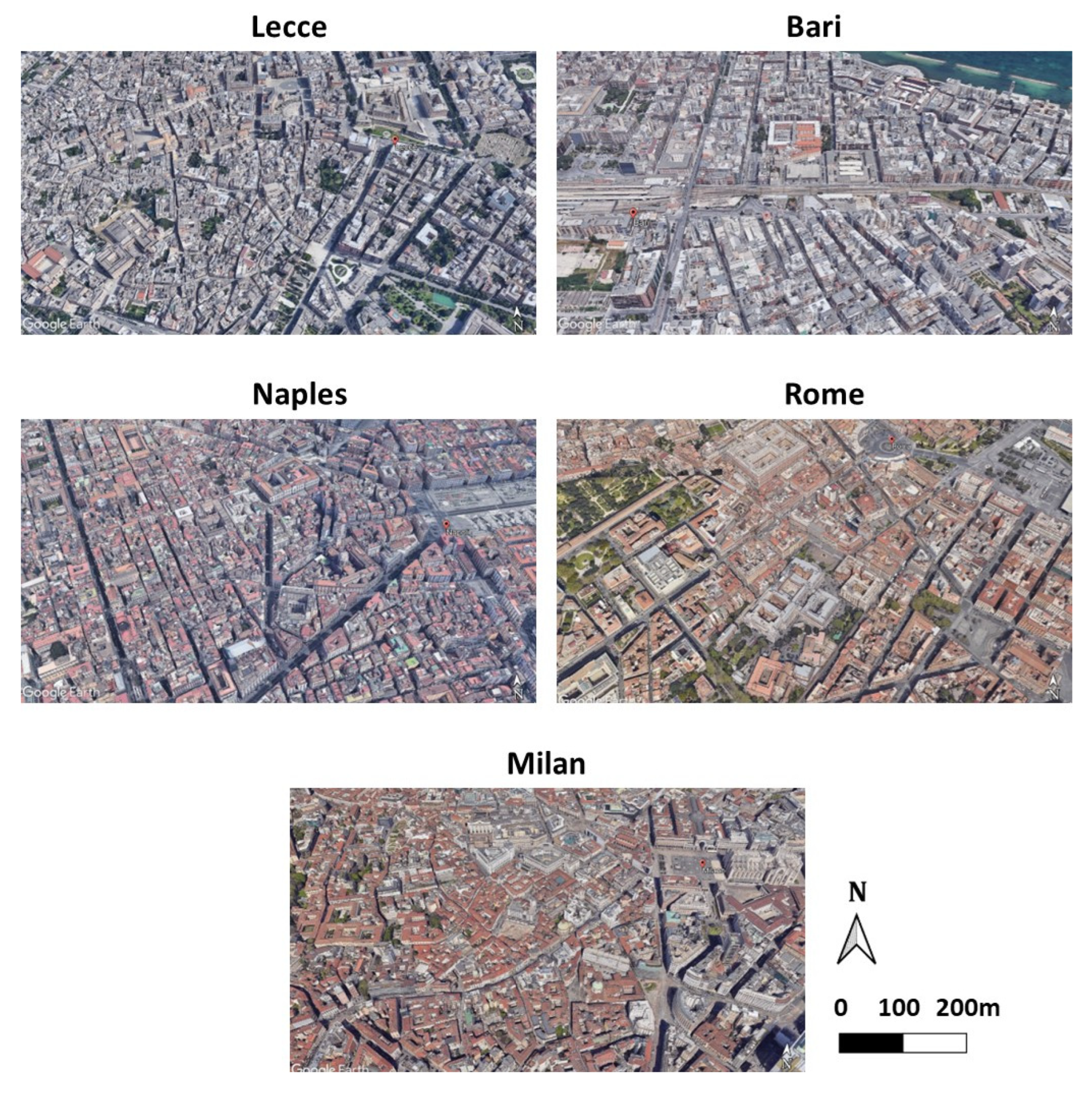
2. Description of the Cities Investigated

Five Italian cities have been considered to conduct the study. Specifically, four metropolitan cities (Article 1, Paragraph 5, Law No. 56/2014; GU Serie Generale n.81 del 07-04-2014, https://www.gazzettaufficiale.it/eli/id/2014/4/7/14G00069/sg, accessed on 23 December 2022) representative of southern, central, and northern Italy have been chosen as they are the largest cities in Italy (https://www.censis.it/sites/default/files/downloads/6_-_Territorio_e_reti_2015.pdf, accessed on 14 December 2022), i.e., Bari (UTM-WGS84: 41°07′31″ N–16°52′00″ E), Naples (40°50′ N–14°15′ E), Rome (41°53′35″ N–12°28′58″ E), and Milan (45°27′40.68″ N–9°09′34.20″ E). The city of Lecce (40°21′07.24″ N–18°10′08.9″ E) has also been chosen, being the home city of the University of Salento. Based on the Köppen Climate Classification, the climate of the cities of Lecce, Naples, and Rome is “Csa” (Mediterranean Climate), characterized by relatively mild winters and very warm summers. The city of Bari is instead characterized by a humid subtropical climate, classified as “Cfa” in the Köppen Climate Classification, and presents relatively high temperatures and evenly distributed precipitation throughout the year. Finally, for the city of Milan, the climate is classified as “Cfb” (Marine West Coast Climate) that is characterized by equable climates with few extremes of temperature and abundant precipitation in all months (https://www.weatherbase.com, accessed on 14 December 2022).

Overall, Milan (1,349,930 inhabitants) (http://dati.istat.it/index.aspx?queryid=19101, accessed on 10 January 2023) shows a radial city development. Relatively new settlements have been built, radiating from the city’s original center. A radial development is also present in Rome (2,749,031 inhabitants), although several nuclei may be distinguished, and the presence of vegetation is more evident. Regarding the city of Lecce (94,783 inhabitants), the radial development starting from the original nucleus occurs along three directions, i.e., the north-west, where there is an industrial area, the east, towards the coast, and the south, where there are mainly residential areas. Finally, Naples (921,142 inhabitants) and Bari (315,948 inhabitants) are both coastal cities. However, while the former developed along the coastline with evident interference from the Vesuvio volcano, the latter expanded inland.

Figure 1 shows the central areas of the five Italian cities selected for the study. Lecce presents a very compact and irregular city center surrounded by compact but regular neighborhoods built in the last decades. Regarding Bari, the compact and irregular old town extends into the sea, while the more recent neighborhoods have been built according to an orthogonal grid. The central area of Naples is very compact and presents both irregular and regular structures. In contrast, the regular and compact structure of the central area of Rome is frequently interrupted by gardens and parks. Finally, Milan exhibits a very compact and irregular structure.

3. Methodology

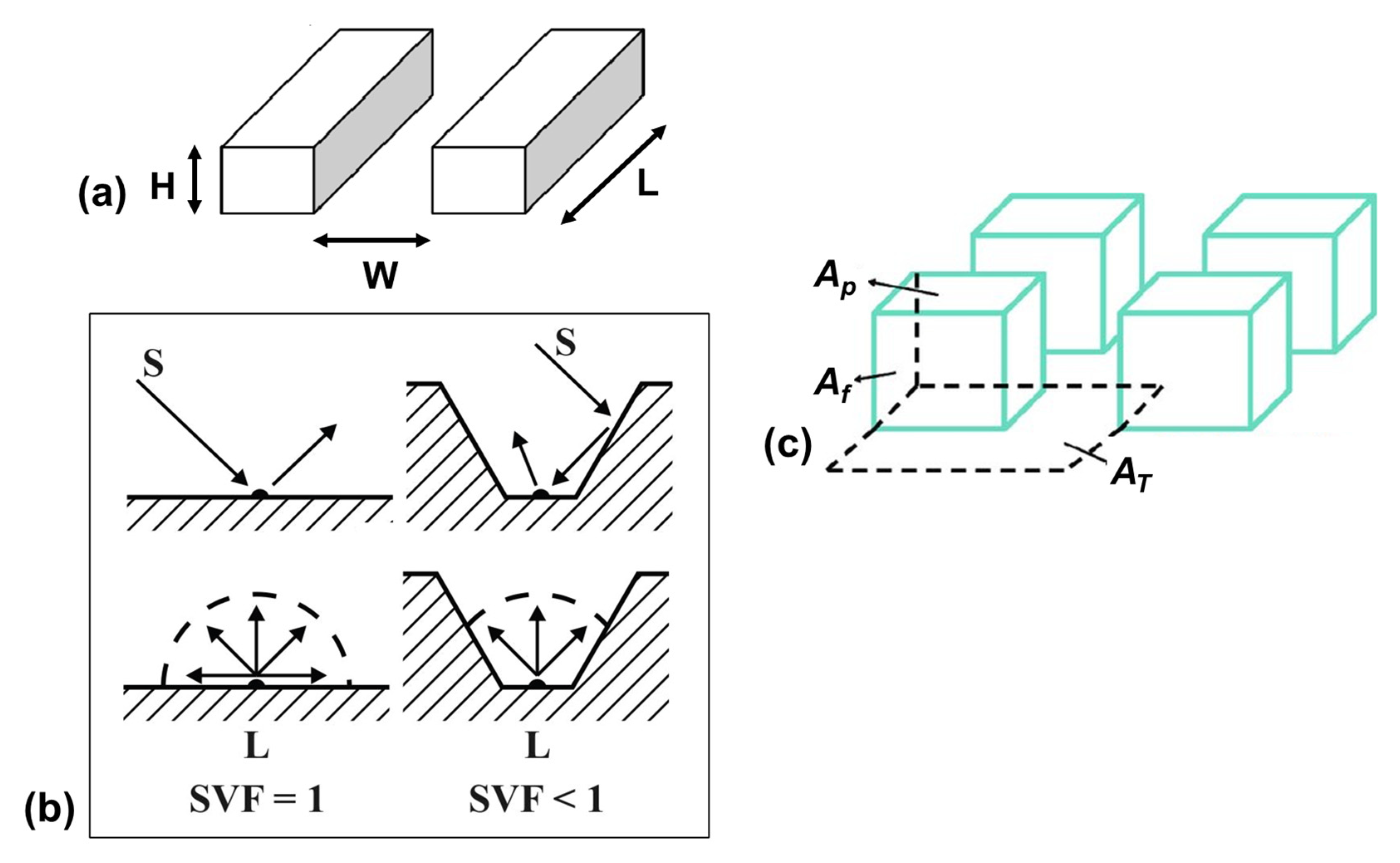
3.1. Description of the Morphological Parameters

Several parameters (Figure 2) have been used to characterize the selected cities:

• mean building height, $\overline{H}$ (m): the geometric average over a specific area of building heights;
• sky view factor, SVF (-): the ratio of the amount of sky hemisphere visible from ground level to that of an unobstructed hemisphere;
• aspect ratio, AR (-): the mean height-to-width ratio of street canyons, building spacing;
• plan area index, λ_p (-): the ratio of building plan area to total plan area.

3.1.1. Mean Building Height

$\overline{H}$ is the average of building height over a specific area:

$$\overline{H}=\frac{{{\displaystyle \sum }}_{i=1}^N{H}_i}{N}$$

(1)

where H_i is the height of building i and N is the total number of buildings in the cell of the grid employed to discretize the city area in GIS (see Section 3.2).

3.1.2. Sky View Factor

The sky view factor (SVF) ranges from 0 to 1, representing totally obstructed and free spaces, respectively; 1 means that all the sky is visible—e.g., it characterizes open land areas—whereas 0 means that the sky is not visible from that specific point. Hence, the lower the SVF, the higher the degree of obstruction in the urban canyon. It is also defined as the ratio of the radiation received (or emitted) by a plan surface to the radiation emitted (or received) by the entire hemispheric environment [29]. Middel et al. [30] have calculated, using a human-centric street canyon perspective in Google Street View, typical SVF footprints for 15 cities around the world. Miao et al. [31] have recently reviewed several methods used to estimate the SVF in urban canyons, outlining their differences, including their respective strengths and weaknesses. In the present work, SVF has been calculated using the Urban Multi-scale Environmental Predictor (UMEP) (https://umep-docs.readthedocs.io/en/latest/index.html, accessed on 14 December 2022). UMEP is a climate service tool designed for researchers and service providers (e.g., architects, climatologists, energy, health, and urban planners) presented as a plugin for QGIS. The Sky View Factor plugin can be used to generate pixel-wise SVF using ground and building models. The methodology that is used to generate SVF in this work is described in Lindberg and Grimmond [32].

3.1.3. Aspect Ratio

The aspect ratio, AR, varies from 0 to more than 2 and represents how narrow the urban canyons are proportional to their height. It may either be computed directly if the average width of urban canyons is known or derived from the sky view factor, SVF. In fact, SVF can also be expressed as SVF = cos (arctan (2*AR)) [33], and, consequently, AR may be expressed as follows:

$$AR=0.5\times \sqrt{{\left(\frac{1}{SVF}\right)}^2-1}$$

(2)

Equation (2) is the one used for performing the present study.

3.1.4. Plan Area Index

The plan area index, λ_p, ranges from 0 to 1 and is defined as the ratio of the plan area of buildings to the total surface area of a specific region:

$${\lambda }_p=\frac{{{\displaystyle \sum }}_{1=1}^N{A}_{pi}}{A_T}$$

(3)

where A_pi is the plan area of the building, i, at ground level, and A_T is the total area of the cell. The values of this parameter depend on the size of the area or of the specific land use types included in the calculation. As reported by Burian et al. [14], in most cases the plan area fraction varies significantly from one city block to the next because of the heterogeneous nature of the urban landscape. The appropriate size of the calculation element should be chosen such that the characteristics of interest in the urban area are homogeneous and discernible.

3.2. Estimation of Morphological Parameters Using GIS

The morphological analyses have been conducted for the selected cities, employing the Geographic Information System (GIS) software QGIS 3.22.1 (https://www.qgis.org/en/site, accessed on 14 December 2022). Hence, morphological and land use data have been collected in shapefiles and analyzed. In addition, for the city of Lecce, the Digital Elevation Model (DEM) has been employed to calculate building heights. Different institutional sources have been used for collecting the relevant data:

• for Lecce and Bari, SIT Puglia (http://www.sit.puglia.it, accessed on 14 April 2022);
• for Naples, Geoportale Nazionale (http://wms.pcn.minambiente.it, accessed on 18 May 2022);
• for Rome Open Data Lazio (https://geoportale.regione.lazio.it, accessed on 20 October 2022);
• for Milan, Milano Geoportale (https://geoportale.comune.milano.it, accessed on 17 June 2022).

Note that a region of interest has been identified for each city selected. The dimensions of the region of interest have been set depending on the selected city size. Therefore, a 10 km × 10 km area has been used for the cities of Lecce and Bari (referred to as “Lecce region” and “Bari region” hereinafter), while a 20 km × 20 km area has been used for the cities of Naples, Rome, and Milan (referred to as “Naples region”, and so on).

Initially, the vector layer containing building footprints and heights has been converted into a raster layer. Then, a vector grid with cells of 100 m × 100 m has been created for the region of interest and used to compute the selected morphological parameters by running zonal statistics functions. The cell size of 100 m × 100 m has been chosen as the theoretically mean smallest relevant spatial unit, where the physical properties of the environment significantly affect air temperatures at the local scale (as reported in Merbitz et al. [34] and Geletič and Lehnert [35]). After the processing, the resulting vector layer has been converted into a raster one.

This process has been applied to calculate each parameter, albeit with slight differences due to various degrees of complexity. Calculating the mean building height has been straightforward: averaging the heights of the buildings in each cell. For the region of Lecce, the mean height has been calculated using the DEM, which has been converted into a raster file containing the shape of the buildings.

In contrast, the calculation of SVF and λ_p has required additional operations, such as creating attributes indicating the presence of buildings in each cell. Finally, the computation of SVF has been more complex and has required more operations. Therefore, a detailed description of the methodology followed for its calculation has been provided in the following subsection.

Specific Case of SVF

For UHI-oriented studies, SVF should be calculated only within urban canyons without considering the building rooftops. The computation has been performed using the UMEP plugin for QGIS. Two raster layers have been employed: the former, called A, reports buildings’ footprint and height, and NoData values have been used to identify the ground. The latter, called B, contains only the buildings’ perimeter. The resolution of the two raster layers has been set to 4 m × 4 m to keep the calculation time acceptable.

To adequately calculate the SVF at the ground level, it is essential to ensure that no values are assigned inside the buildings. The first step is to calculate the difference between the two rasters B and A to obtain a new raster, C. In the new raster, negative values are inside the buildings and NoData values correspond to ground/streets. In the second step, the NoData values have been converted into zeros. In the third step, raster C is summed to raster B to obtain a new raster, D. D ranges from – (max height) to + (max height). In the fourth step, the negative values in raster D, corresponding to pixels inside the buildings, have been replaced by NoData values. Consequentially, a raster layer is created with zeros for the ground and NoData values for the pixels inside the buildings, and height information is reported along the building contours. It should be noted that the NoData values of pixels inside the buildings include the rooftops.

Once the fourth step has been completed, it is possible to compute SVF by employing a function embedded in the UMEP plugin, i.e., sky view factor. The resulting raster (called E) still includes SVF values for contours and the inside of the buildings, which must be removed. Therefore, a comparison of raster E with raster D has enabled the replacement of the SVF data (for the inside of the buildings) with NoData. Finally, to remove the SVF data on the contours, a negative of the contour lines raster (neg_B) has been created with NoData on the contours, and 0 everywhere else. Comparing raster neg_B with raster E, the SVF data have thus been removed from the contour lines in raster E.

Finally, the obtained object is a raster with SVF values everywhere (except in the buildings), which has been processed using the zonal mean statistics function over the 100 m × 100 m grid as performed for the other morphological parameters.

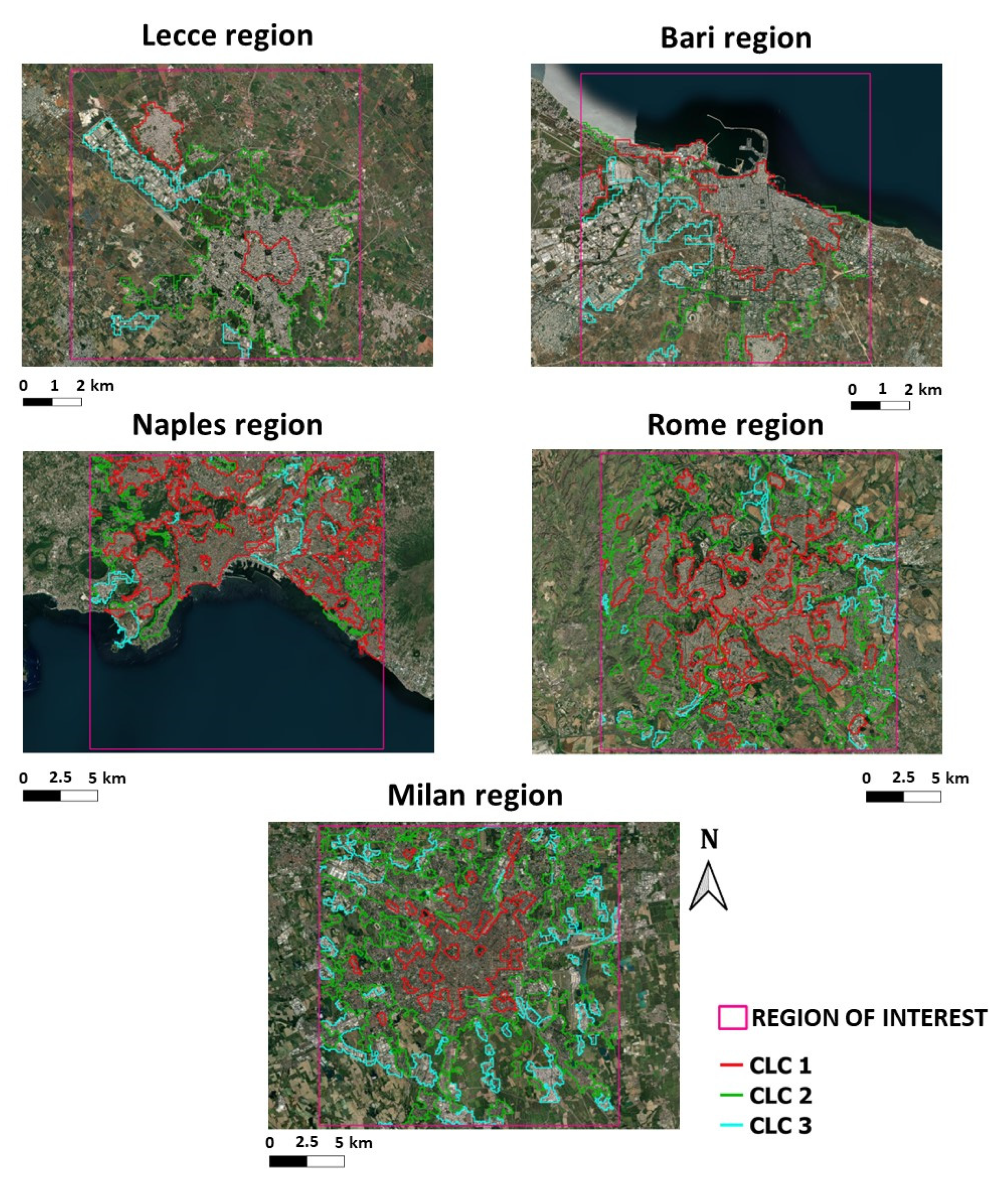
3.3. Data Analysis Based on CORINE Land Cover Classes

In order to ease the comparison between the different cities taking into account their main characteristics in terms of land cover, Corine Land Cover (CLC) classes have been used. The Corine (Coordination of Information on the Environment) Land Cover project provides information on the biophysical characteristics of European land cover. The CLC project was established in the 1980s to standardize data collection on the state of land in Europe and to support environmental policy and has become the primary spatial data source on land for the European Economic Area. Images are acquired by earth observation satellites. It is currently a product of the Copernicus Land Monitoring Service. Copernicus is the earth observation program of the European Union (https://collections.eurodatacube.com/, accessed on 14 December 2022). The CLC inventory consists of 44 land cover and land use classes derived from satellite data.

For the present study, the three main CLC classes present in the cities have been considered: 1.1.1, 1.1.2, and 1.2.1, which stand for “continuous urban fabric” (hereafter CLC 1), “discontinuous urban fabric” (hereafter CLC 2), and “industrial or commercial units” (hereafter CLC 3), respectively (Figure 3) (https://land.copernicus.eu/pan-european/corine-land-cover, accessed on 14 December 2022).

CLC 1 is assigned when urban structures and transport networks are predominant: above 80% of the land surface is covered by impermeable features such as buildings, roads, and artificially surfaced areas. Non-linear areas of vegetation and bare soil are exceptional. CLC 2 is assigned when urban structures and transport networks associated with vegetated areas and bare surfaces are present and occupy significant surfaces in a discontinuous spatial pattern. Impermeable features such as buildings, roads, and artificially surfaced areas range from 30 to 80% land coverage. In CLC 3, buildings, other built-up structures, and artificial surfaces (with concrete, asphalt, tarmacadam, or stabilized, e.g., beaten earth) occupy most of the area. It can also contain vegetation (most likely grass) or other non-sealed surfaces. This class is assigned for land units that are under industrial or commercial use or serve for public service facilities (https://land.copernicus.eu/user-corner/technical-library/corine-land-cover-nomenclature-guidelines/html/index.html, accessed on 14 December 2022).

Once the Corine Land Cover raster (https://land.copernicus.eu/pan-european/corine-land-cover/clc2018, accessed on 3 November 2022) has been imported in QGIS, a vector layer has been created for each of the selected CLC classes. The zonal “majority” statistical function has been used to obtain values of morphological parameters over the grid of each CLC class. The obtained data have then been extracted to calculate the statistics (in terms of spatial averages and standard deviations) for each CLC class.

4. Results and Discussion

This section reports and discusses the results of the morphological analyses performed for the five cities in the regions of interest. In Section 4.1, the results are presented in terms of λ_p and $\overline{H}$ using maps. These two parameters have been selected because they quantify the pressure on the environment of the selected built areas. Comparing building height and plan area density distributions may characterize qualitatively and quantitatively the differences between the selected regions. The morphological characteristics are analyzed separately for each region, and then a cross-comparison is performed. In Section 4.2, the results are referred to the three specific CLCs and are presented using tables. Please note that each value in the table is calculated as the spatially-averaged value over the entire area of the specific CLC for each region. Limitations and future perspectives are given in Section 4.3. Section 4.4. finally reports on an example of an atmospheric-oriented application of the morphological parameters, specifically the building of a detailed LCZ map (for the Lecce region).

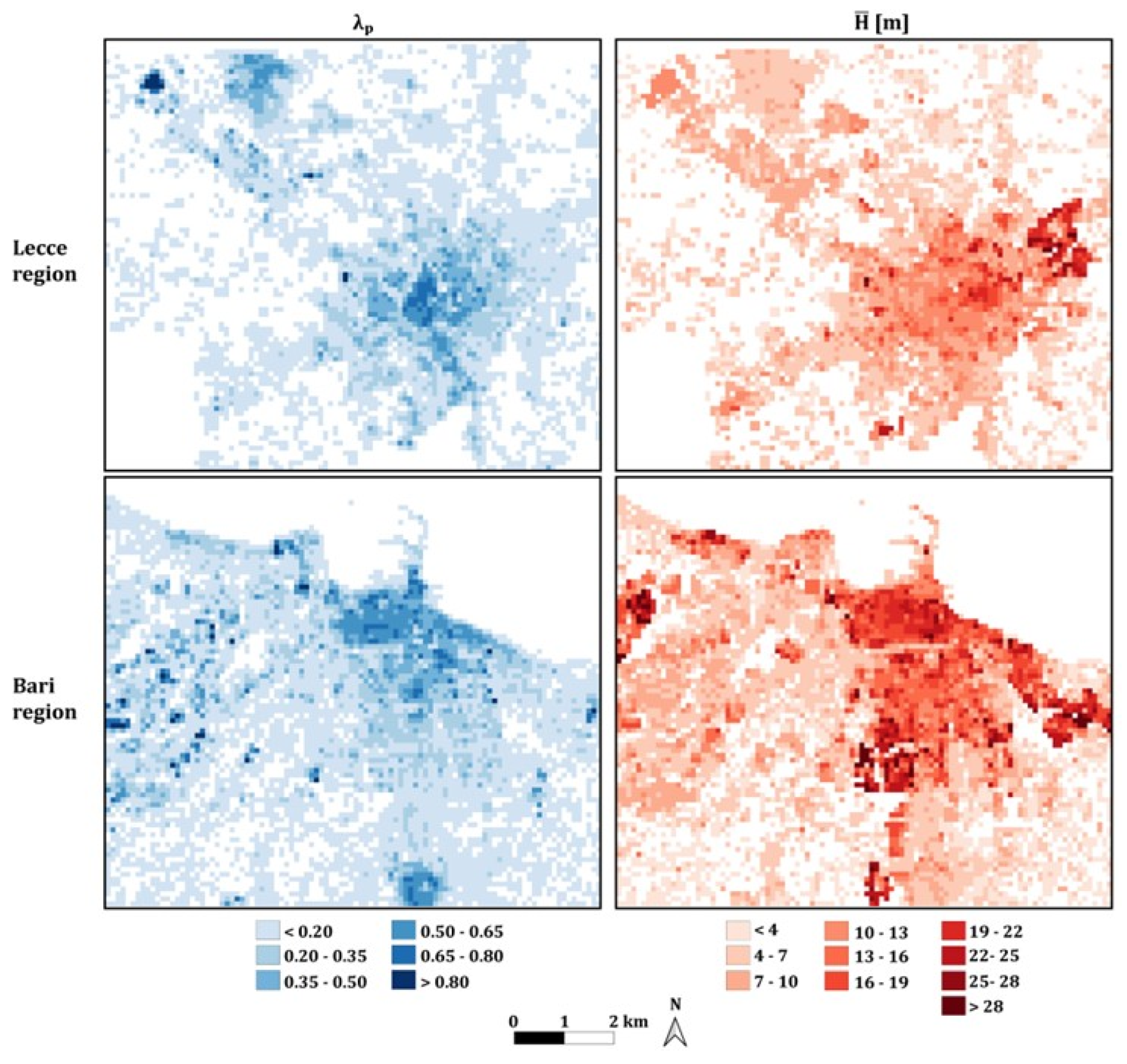
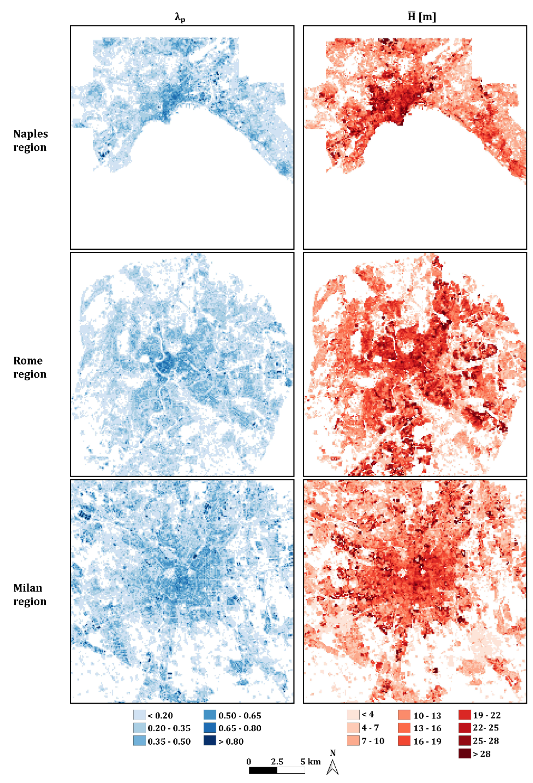
4.1. Morphological Parameter Maps

Figure 4 and Figure 5 show the maps of $\overline{H}$ and λ_p of the five selected regions. Further,

Table 1. Spatially-averaged, median and maximum values of the morphological parameters over the whole region.

	Spatially-Averaged		Median		Max
Region	$\overline{\mathit{H}}$ (m)	λp (-)	$\overline{\mathit{H}}$ (m)	λp (-)	$\overline{\mathit{H}}$
Lecce	7.1	0.14	5.9	0.07	30.9
Bari	8.8	0.16	6.5	0.10	47.3
Naples	12.0	0.20	11.0	0.16	76.7
Rome	12.7	0.19	11.8	0.16	73.5
Milan	10.9	0.22	9.1	0.19	79.3

reports the spatially-averaged and median values of $\overline{H}$ and λ_p and the maximum values of $\overline{H}$.

Figure 4 reports the maps of Lecce and Bari regions. Regarding the Lecce region, the Lecce city center and the northwestern part of the city present the highest values of λ_p (0.25–0.80), while the highest values of $\overline{H}$ (above 28 m) are mainly located in the northeastern part. Spatially-averaged values equal to 0.14 (λ_p) and 7.1 m ($\overline{H}$) and median values equal to 0.07 and 5.9 m are found for the whole region. Regarding the Bari region, the Bari city center presents the highest values of λ_p (0.50–0.65), with the highest values of $\overline{H}$ (above 28 m) mostly located in the central and eastern parts and, to a lesser extent, in the western sector of the city. Spatially-averaged values equal to 0.16 (λ_p) and 8.8 m ($\overline{H}$) and median values equal to 0.10 and 6.5 m are found.

Figure 5 shows the maps of the Naples, Rome, and Milan regions. The Rome region is characterized by a decreasing trend of λ_p from the Rome city center (0.65–0.80) to the outskirts (0.20–0.35). In the whole region, λ_p shows a spatially-averaged value of 0.19 and a median value of 0.16, while $\overline{H}$ presents a spatially-averaged value of 12.7 m and a median value of 11.8 m. Finally, the city center is also the area with the highest values of $\overline{H}$, which is above 20 m. In the Naples region, λ_p presents a spatially-averaged value of 0.20 and a median value of 0.16, while the highest values are found in the city center, where λ_p ranges between 0.65 and 0.80. Furthermore, the area close to the sea presents $\overline{H}$, ranging from 25 m to 28 m, while a spatially-averaged value of 12.0 m and a median value of 11.0 m are obtained for the whole region. Finally, in the Milan region, λ_p presents a spatially-averaged value equal to 0.22 and a median value equal to 0.19, while the highest values occur in the Milano city center, where λ_p ranges between 0.65 and 0.80. Furthermore, the city center presents $\overline{H}$ ranging from 13 m to 20 m, while the highest values (above 28 m) are scattered outside the center. In addition, $\overline{H}$ shows a spatially-averaged value of 10.9 m and a median value of 9.1 m.

Overall, from the analysis of the maps and associated spatially-averaged and median values, it can be argued that there is a gradual increase in λ_p moving from the south to the north of Italy, with the highest spatially-averaged values found in Milan (0.22), Rome (0.19), and Naples (0.20) regions. The Rome region also shows the highest spatially-averaged $\overline{H}$ (12.8 m), followed by the Naples (11 m) and Milan (10.9 m) regions. In addition, in terms of maximum values of $\overline{H}$ located in the city centers, the three regions have the highest values. As for the southern regions, both show similar spatially-averaged values, which are slightly larger in the Bari (0.16 for λ_p and 8.8 m for $\overline{H}$) region than in the Lecce (0.14 for λ_p and 7.1 m for $\overline{H}$) region.

Finally, it is interesting to note that the city of Lecce and, to a lesser extent, Milan has a symmetrical spatial distribution of λ_p and $\overline{H}$, with higher values in the city center and decreasing symmetrically moving towards the periphery. On the other hand, the two coastal cities, Bari and Naples, show higher values near the coast, with values gradually decreasing away from the coast. Finally, Rome shows a particular distribution, with higher values in the city center and along spatial radii stretching in all directions, while the values are lower elsewhere.

Results obtained for the investigated cities agree with values found in the literature for other Italian cities. For example, Giovannini et al. [25] and Pappaccogli et al. [26] have obtained a similar range of λ_p for the cities of Trento and Bolzano. Similarly, Di Sabatino et al. [24] have analyzed three different urbanized neighborhoods of the city of Lecce and found values of λ_p equal to approximately 0.40, in line with the results achieved in this paper.

4.2. Comparison of the Morphological Characteristics

Table 2. Spatially-averaged values and standard deviations of the morphological parameters over the CLC 1 area.

CLC 1	Spatially-Averaged				St. Dev.
Region	$\overline{\mathit{H}}$ (m)	AR (-)	SVF (-)	λp (-)	$\overline{\mathit{H}}$ (m)	AR (-)	SVF (-)	λp (-)
Lecce	9.5	0.53	0.75	0.34	4.3	0.37	0.19	0.19
Bari	14.1	0.60	0.69	0.32	6.2	0.41	0.20	0.18
Naples	15.2	0.50	0.74	0.26	6.9	0.40	0.20	0.16
Rome	16.4	0.63	0.67	0.28	6.1	0.40	0.20	0.14
Milan	16.0	0.68	0.63	0.36	5.6	0.32	0.17	0.15

,

Table 3. Spatially-averaged values and standard deviations of the morphological parameters over the CLC 2 area.

CLC 2	Spatially-Averaged				St. Dev.
Region	$\overline{\mathit{H}}$ (m)	AR (-)	SVF (-)	λp (-)	$\overline{\mathit{H}}$ (m)	AR (-)	SVF (-)	λp (-)
Lecce	8.5	0.26	0.88	0.17	4.8	0.22	0.12	0.14
Bari	10.0	0.22	0.90	0.13	7.9	0.15	0.09	0.12
Naples	10.5	0.22	0.90	0.13	5.3	0.18	0.11	0.10
Rome	12.5	0.25	0.88	0.16	6.8	0.22	0.13	0.11
Milan	11.6	0.31	0.84	0.20	7.2	0.22	0.14	0.14

and

Table 4. Spatially-averaged values and standard deviations of the morphological parameters over the CLC 3 area.

CLC 3	Spatially-Averaged				St. Dev.
Region	$\overline{\mathit{H}}$ (m)	AR (-)	SVF (-)	λp (-)	$\overline{\mathit{H}}$ (m)	AR (-)	SVF (-)	λp (-)
Lecce	7.4	0.11	0.96	0.16	3.3	0.11	0.06	0.19
Bari	7.1	0.18	0.93	0.19	3.1	0.12	0.07	0.19
Naples	9.7	0.19	0.92	0.22	5.3	0.16	0.10	0.20
Rome	8.3	0.12	0.95	0.20	4.2	0.14	0.08	0.18
Milan	9.3	0.22	0.90	0.25	6.2	0.16	0.10	0.20

report the spatially-averaged values, over the entire CLC area, of each parameter and the standard deviations. Please note that CLCs represent homogeneous areas that are mostly covered by buildings or artificial structures (CLC 1 and CLC 3) or a mixture of buildings and vegetated areas. Spatially-averaged values over each CLC thus do not expressively refer to whole non-built-up areas.

Regarding CLC 1, moving from southern to northern cities, there is a gradual increase in $\overline{H}$, with the Rome and Milan regions showing the highest spatially-averaged values (16.4 m and 16.0 m, respectively). AR and SVF, on the other hand, do not follow the same decreasing (for AR) or increasing (for SVF) trends from southern to northern cities as the increasing trend found for $\overline{H}$. The Naples and Lecce regions present the lowest AR (0.50 and 0.453, respectively) and the highest SVF (0.74 and 0.75, respectively), while the Milan region shows the highest AR (0.68) and the lowest SVF (0.63). Low values of AR and high values of SVF are related to urban configurations with low values of λ_p. In fact, the Naples region shows the lowest plan area density among the investigated cities (0.26), while the Milan region shows the highest one (0.36), followed by the Lecce (0.34) and Bari (0.32) regions. The Naples and Rome regions are instead characterized by the lowest values (0.26 and 0.28, respectively). It is interesting to note that the Lecce region, even though characterized by the lowest $\overline{H}$ (9.5 m), presents a high value of λ_p (0.34), which is likely due to the fact that CLC 1 mainly covers the compact city center (Figure 3) and not further surrounding areas, as occurs for the other regions. Note that this value confirms the definition of Lecce as a compact city and is in line with the values found by Di Sabatino et al., where three neighborhoods of Lecce were analyzed [24].

Regarding CLC 2, similarly to CLC 1, there is a gradual increase in $\overline{H}$ moving from the south to the north of Italy, with the Rome and Milan regions showing the highest spatially-averaged values (12.5 m and 11.6 m, respectively) and high standard deviations. Moreover, the two regions present similar values of AR (0.25 and 0.31, respectively) and SVF (0.88 and 0.84, respectively). Finally, λ_p is the highest (0.20) in the Milan region, followed by the Lecce region, with 0.17.

As expected, CLC 3 presents for each city region the lowest values of $\overline{H}$ and AR and the largest values of SVF. Regarding $\overline{H},$ the Naples region presents the highest value, while the Bari region shows the lowest. The Milan region, similar to what occurs in CLC 1 and CLC 2, still shows the highest AR (0.22) and λ_p (0.25), followed by the Napoli region (0.19 for AR and 0.22 for λ_p). It should be noted that spatially-averaged values and standard deviations of λ_p are slightly larger than those found in CLC 2, but for Lecce, which, given its geometrical symmetrical distribution, shows a symmetrical distribution of λ_p.

Comparing the three CLCs, as expected from their definition, the quantitative morphological analysis performed here confirms that, for all the city regions, CLC 1 areas (continuous urban fabric) are those with the highest urbanization, with medium SVF values and λ_p values typical of compact cities [36,37], characterized by wake interference or skimming flow regimes [38]. In CLC 2 areas, the plan area density decreases, presenting values typical of sparse cities characterized by isolated roughness or wake interference flow regimes. Finally, results for CLC 3 confirm a decrease in $\overline{H}$ and AR moving from the city center, but with larger λ_p than CLC 2. This is because CLC 2 includes impermeable features covering 30 to 80% of the land, while in CLC 3 built-up structures and artificial surfaces occupy most of the area.

4.3. Limitations and Future Morphological Works

An advantage of the methodology presented in this paper is that it employs only two sets of input data (building heights and grid maps) based on the actual shape of buildings to calculate the morphological parameters of a given city or region. Hence, for its application, it is necessary to collect appropriate and accurate datasets of building geometry to apply zonal statistical functions and calculate morphological parameters.

Looking at Figure 4 and Figure 5 and Table 2, Table 3 and Table 4, larger spatially-averaged values can be expected in the tables, especially for AR and λ_p for the Naples, Rome, and Milan regions in CLC 1. First, it should be noted that results do not refer only to the city but to a region of 20 km × 20 km that includes, in some cases, nearby towns, which are less dense than the main city. Furthermore, a minimum mapping unit (MMU) of 25 ha for areal phenomena and a minimum width of 100 m for linear phenomena have been used for obtaining the CLC in the Corine project. In addition, high-resolution satellite imagery is mainly processed by visual interpretation. Boundaries of a specific class may thus cover zones that do not belong appropriately to that class. This aspect has affected the spatially-averaged values of morphological parameters over a given CLC, as shown in Table 2, Table 3 and Table 4.

A grid sensitivity test has been performed using several grid resolutions: 50 m × 50 m, 250 m × 250 m, 500 m × 500 m, and 1000 m × 1000 m. The calculation has been performed for the Lecce region, and the results are shown in

Table 5. Spatially-averaged values and standard deviations of the morphological parameters for the three CLCs for the Lecce region using different grid resolutions.

Lecce Region	Spatially-Averaged				St. Dev.
CLC 1	$\overline{\mathit{H}}$ (m)	AR (-)	SVF (-)	λp (-)	$\overline{\mathit{H}}$ (m)	AR (-)	SVF (-)	λp (-)
50 m × 50 m	9.53	0.62	0.72	0.37	4.53	0.54	0.22	0.21
100 m × 100 m	9.45	0.53	0.75	0.34	4.26	0.42	0.19	0.19
250 m × 250 m	9.14	0.42	0.79	0.29	3.86	0.33	0.16	0.17
500 m × 500 m	9.31	0.39	0.82	0.28	3.29	0.27	0.15	0.16
1000 m × 1000 m	9.08	0.31	0.85	0.23	2.68	0.21	0.11	0.12
CLC 2
50 m × 50 m	8.74	0.30	0.86	0.22	5.10	0.27	0.15	0.17
100 m × 100 m	8.51	0.26	0.88	0.17	4.76	0.22	0.12	0.14
250 m × 250 m	8.04	0.21	0.90	0.13	3.74	0.20	0.11	0.12
500 m × 500 m	7.68	0.18	0.92	0.11	3.29	0.19	0.10	0.12
1000 m × 1000 m	7.93	0.15	0.93	0.10	2.87	0.16	0.08	0.11
CLC 3		AR (-)
50 m × 50 m	7.65	0.15	0.95	0.25	3.41	0.15	0.08	0.27
100 m × 100 m	7.34	0.11	0.96	0.16	3.33	0.11	0.06	0.19
250 m × 250 m	7.10	0.08	0.97	0.09	2.83	0.07	0.03	0.11
500 m × 500 m	7.10	0.06	0.98	0.07	2.57	0.05	0.02	0.07
1000 m × 1000 m	7.67	0.07	0.97	0.06	2.27	0.06	0.03	0.04

. Taking into account values for the 100 m × 100 m grid resolution as a reference, the table shows that:

• moving from the coarser (1000 m × 1000 m) to the finer (50 m × 50 m) grid resolutions, values of $\overline{H}$, AR, and λ_p increase, while values of SVF decrease;
• the maximum percentage deviations obtained using the finer grid (50 m × 50 m) are 16% (for AR in CLC 1) and 26% (for λ_p in CLC 2). On the other hand, the deviations obtained using the other grid resolutions (250 m × 250 m, 500 m × 500 m, and 1000 m × 1000 m) are in general larger than those obtained using 50 m × 50 m;
• focusing on values obtained for CLC 3, larger deviations (than those found for CLC 1 and 2) can be noted using the 50 m × 50 m grid resolution, with a maximum deviation of 60% for λ_p. This may be due to the small grid cells (50 m × 50 m), which experience a larger number of values close to 0 (cell without buildings) and 1 (cell fully occupied by buildings) as confirmed by the high standard deviation.

These preliminary results suggest that using a grid resolution finer than 50 m × 50 m will produce lower differences with respect to the 100 m × 100 m grid resolution and thus building a dataset of parameters averaged over cells of 100 m × 100 m may be an appropriate compromise to calculate parameters over large areas. These preliminary findings will be explored in future work, performed by conducting the grid sensitivity test to the other regions of the cities investigated.

Finally, it is worth mentioning that there are several methods in the literature for calculating SVF [31]. An additional aspect of future work is to test the accuracy of the different methods in QGIS.

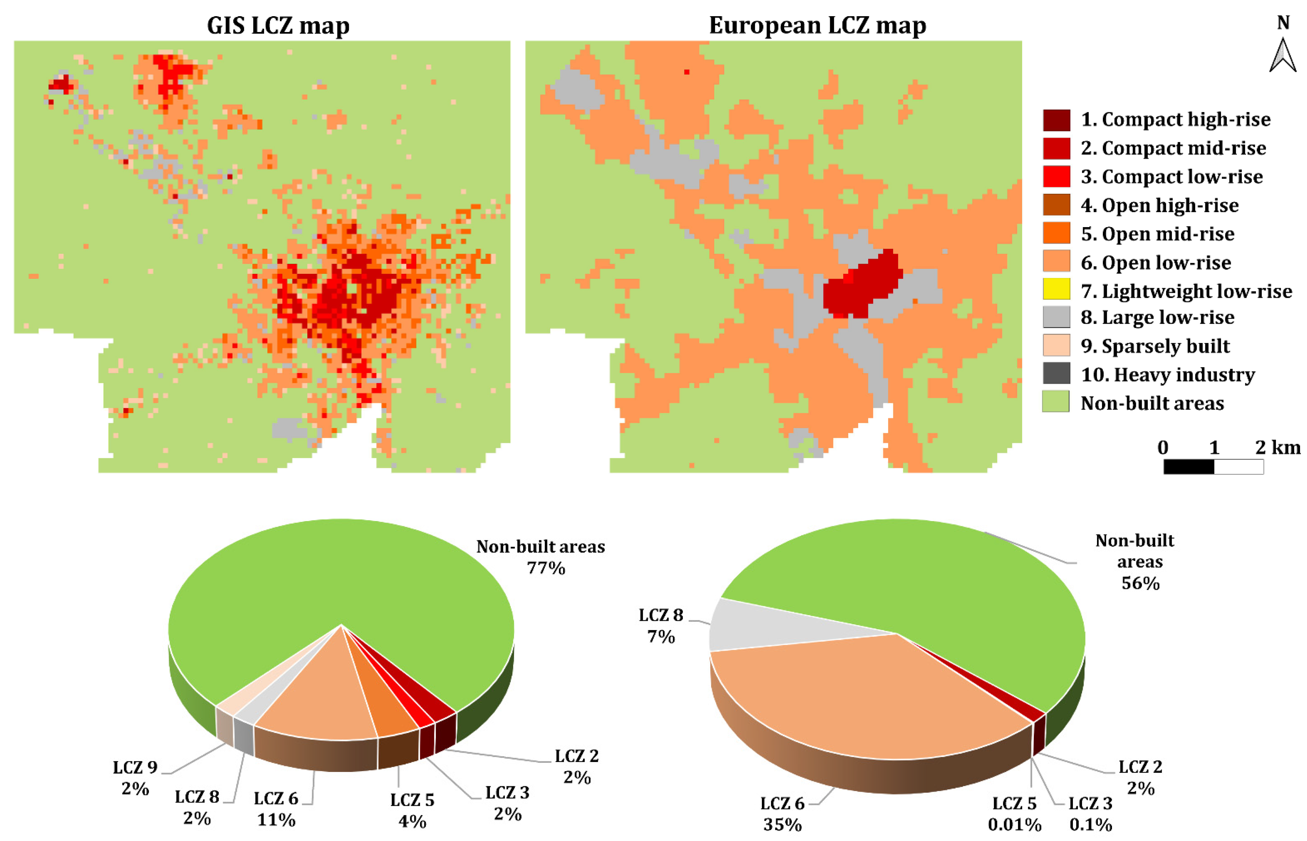
4.4. LCZ Map Based on Morphological Parameters

The calculated morphological parameters can be used to build detailed LCZ maps. Here, as an example, the map of the Lecce region is presented and discussed. As mentioned in the Introduction, the concept of LCZ contributed to an advancement in the thermal analysis of urban areas. Thermal differences, for example in UHI intensities, are no longer confined to urban/rural temperature differences, but they can also be analyzed more closely as differences between LCZs. Thus, the LCZ scheme is a useful tool to compare the thermal features of various neighborhoods within a city, and/or similar neighborhoods between different cities. The LCZ concept has been applied in a wide range of urban climate investigations [39].

As mentioned above, each LCZ is characterized by different morphological and surface cover properties. The morphological parameters are $\overline{H},$SVF, AR, λ_p, impervious surface fraction, pervious surface fraction, and terrain roughness class [15]. There are three different levels of LCZ maps. The World Urban Database and Access Portal Tools (WUDAPT, www.wudapt.org, accessed on 19 December 2022), which uses freely available Landsat imagery and Google Earth for creating the training areas (TAs), provides a procedure for generating the LCZ level 0 product. Level 0 represents the first level of information, while Levels 1 and 2 provide more detailed information [40]. The European LCZ level 0 map from Demuzere et al. [41] is available for download as a GeoTiff at the WUDAPT database. There are other approaches for generating LCZ level 0 products that can also lead to detailed Level 1 and 2 data. Where the data are available, administrative data (on building footprints, heights, green spaces, etc.) and GIS can be used (e.g., [19,35,42,43]), as performed here.

Specifically, for building the LCZ map (GIS LCZ map hereinafter) of the Lecce region, all the morphological parameters given by Stewart and Oke [15] have been calculated, except for the roughness class. The GIS LCZ map has then been built considering Stewart and Oke’s criterions and employing fuzzy logic to determine the three most probable LCZ for every cell [44]. A grid of 100 m × 100 m cells has been thus obtained, each cell containing those three most probable LCZs. The corresponding map (with only the most probable LCZ drawn) can be seen in Figure 6, which also shows the European LCZ map for comparison. Please note that no fuzzy logic has been used for the pervious surface fraction, used at the beginning of the script to distinguish between urban and non-urban areas, with a threshold at 80% (this choice is a main source of inaccuracy). In the GIS LCZ map, as information on the Land Cover Types (LCZ A, B, C, D, E, F, and G) was missing, all these classes were grouped in a single class called Non-built areas and, for consistency, the same was done for the European LCZ map.

The European LCZ map shows that LCZ 6 (Open low-rise) is the most abundant (35%), characterizing the city outskirts. The city center is characterized by LCZ 2 (Compact mid-rise), while all around the center and in the north-western part of the city there is the presence of LCZ 8 (Large low-rise), the latter corresponding to the industrial/commercial zone of Lecce city. When compared with the GIS LCZ map, it can be noted that the area covered by LCZ 2 is the same (6%), even though more irregularly distributed throughout the region. It is noteworthy that the LCZ 6 now covers 11% of the area; in fact, areas around the center are now mostly reclassified as LCZs 5 (Open mid-rise) and 6, while the LCZ 8 area is reduced and mostly appears in the northern/western part as in the European map. Finally, scattered areas of LCZ 9 (Sparsely built) appears.

To assess the classification accuracy of both the GIS-based and WUDAPT methods, a confusion matrix was produced by comparing the European map to the GIS map. As an example, the overall accuracy (OA) has been calculated as follows [20]:

$$OA=\frac{{{\displaystyle \sum }}_{i\in LCZ}{x}_{i,i}}{total pixel numbers}$$

(4)

OA is a statistic representing the proportion of pixels that were classified in the same way by both maps, and it is shown in the form of a percentage. An overall accuracy of 73% has been found.

In summary, while the general spatial distribution patterns of different LCZ classes in the two LCZ maps are qualitatively similar (Figure 6), the GIS-based method can improve the accuracy because the WUDAPT L0 method misclassified some LCZs, especially at the core urban cells. On the other hand, the WUDAPT method generates LCZ maps with a more homogeneous pattern than the GIS-based method. Findings from this work can provide a useful reference for researchers who are interested in LCZ classification and mapping work for their cities. Further analysis will be performed in the future to compare the methods, improve the GIS-based method in classifying the zones, and also consider surface cover properties to improve the overall LCZ classification. The same will be applied to the other regions analyzed in the present paper.

5. Conclusions

Morphological analyses have been conducted for five cities characterized by different climate, structure, and size, located in southern (Lecce and Bari), central (Naples and Rome), and northern (Milan) Italy. The calculation of four morphological parameters, namely mean building height, sky view factor, aspect ratio, and plan area index, has been performed using the GIS software QGIS. The methodology employs only two sets of data as input, i.e., building heights and footprints, and is based on the creation of a vector grid covering the study area to compute zonal statistics thanks to the appropriate module of QGIS. This methodology can be replicable in other urban contexts.

Results have been presented in maps for selected regions of interest, including the cities and the respective surrounding areas. A gradual increase in the plan area index moving from the south to the north of Italy has been obtained. Following the geometrical structure of the city, Lecce and, to a lesser extent, Milan have shown a symmetrical spatial distribution of planar area index and mean building height, with higher values in the city centers. On the other hand, the two coastal cities, Bari and Naples, have shown higher values near the coast, with values gradually decreasing away from the coast. Rome is instead characterized by higher values in the city center and along spatial radii stretching in all directions.

In addition, the morphological parameters have been spatially averaged over three specific CLCs, confirming that CLC 1 areas (continuous urban fabric) have the highest urbanization, with medium sky view factor values and plan area index values typical of compact cities. At the same time, CLC 2 and CLC 3 areas have shown values typical of sparse cities.

Results suggest that it is possible to build datasets of morphological parameters averaged over a grid of a chosen resolution (100 m × 100 m in this case), which can be employed to calculate the parameters over wider areas. The methodology followed here can represent the first step towards (i) building LCZ maps of levels 1 and 2, as performed in this paper for the Lecce region, useful for UHI/microclimate studies; and (ii) developing parameterizations for mesoscale models to represent the dynamic effect of urban areas.

References

1. Hilber, C.; Palmer, C. Urban Development and Air Pollution: Evidence from a Global Panel of Cities. Grantham Research Institute on Climate Change and the Environment, Working Paper No. 175. 2014. Available online: http://www.lse.ac.uk/GranthamInstitute/wp-content/uploads/2014/12/Working-Paper-175-Hilber-Palmer-2014.pdf (accessed on 1 December 2022).
2. Kim, S.W.; Brown, R.D. Urban heat island (UHI) intensity and magnitude estimations: A systematic literature review. Sci. Total Environ. 2021, 779, 146389. [Google Scholar] [CrossRef] [PubMed]
3. Britter, R.E.; Hanna, S.R. Flow and dispersion in urban areas. Annu Rev. Fluid Mech. 2003, 35, 469–496. [Google Scholar] [CrossRef]
4. Ferreira, D.G.; Diniz, C.B.; de Assis, E.S. Methods to calculate urban surface parameters and their relation to the LCZ classification. Urban Clim. 2021, 36, 100788. [Google Scholar] [CrossRef]
5. Palusci, O.; Cecere, C. Urban Ventilation in the Compact City: A Critical Review and a Multidisciplinary Methodology for Improving Sustainability and Resilience in Urban Areas. Sustainability 2022, 12, 44. [Google Scholar] [CrossRef]
6. Di Sabatino, S.; Buccolieri, R.; Pappaccogli, G.; Leo, L.S. The effects of trees on micrometeorology in a real street canyon: Consequences for local air quality. Int. J. Environ. Pollut. 2015, 58, 100–111. [Google Scholar] [CrossRef]
7. Li, Z.; Ming, T.; Liu, S.; Peng, C.; de Richter, R.; Li, W.; Zhang, H.; Wen, C.-Y. Review on pollutant dispersion in urban areas-part A: Effects of mechanical factors and urban morphology. Build. Environ. 2021, 190, 107534. [Google Scholar] [CrossRef]
8. Buccolieri, R.; Carlo, O.S.; Rivas, E.; Santiago, J.L.; Salizzoni, P.; Siddiqui, M.S. Obstacles influence on existing urban canyon ventilation and air pollutant concentration: A review of potential measures. Build. Environ. 2022, 214, 108905. [Google Scholar] [CrossRef]
9. Wu, M.; Zhang, G.; Wang, L.; Liu, X.; Wu, Z. Influencing Factors on Airflow and Pollutant Dispersion around Buildings under the Combined Effect of Wind and Buoyancy—A Review. Int. J. Environ. Res. Public Health 2022, 19, 12895. [Google Scholar] [CrossRef]
10. Peng, Y.; Buccolieri, R.; Gao, Z.; Ding, W. Indices employed for the assessment of “urban outdoor ventilation”—A review. Atmosph. Envir. 2020, 223, 117211. [Google Scholar] [CrossRef]
11. Martilli, A.; Clappier, A.; Rotach, M.W. An urban surface exchange parameterisation for mesoscale models. Bound.-Layer Meteorol. 2002, 104, 261–304. [Google Scholar] [CrossRef]
12. Buccolieri, R.; Santiago, J.L.; Martilli, A. CFD modelling: The most useful tool for developing mesoscale urban canopy parameterizations. Build. Simul. 2021, 14, 407–419. [Google Scholar] [CrossRef]
13. Grimmond, C.S.B.; Oke, T.R. Aerodynamic Properties of Urban Areas Derived from Analysis of Surface Form. J. Appl. Meteorol. Climatol. 1999, 38, 1262–1292. [Google Scholar] [CrossRef]
14. Burian, S.; Augustus, N.; Jeyachandran, I.; Brown, M. National Buildings Statistics Database: Version 2; LA-UR-08-1921; University of Utah: Salt Lake City, Utah, USA, 2008; p. 82. [Google Scholar]
15. Stewart, I.D.; Oke, T.R. Local climate zones for urban temperature studies. Bull. Am. Meteorol. Soc. 2012, 93, 1879–1900. [Google Scholar] [CrossRef]
16. Feng, W.; Liu, J. A Literature Survey of Local Climate Zone Classification: Status, Application, and Prospect. Buildings 2022, 12, 1693. [Google Scholar] [CrossRef]
17. Palusci, O.; Monti, P.; Cecere, C.; Montazeri, H.; Blocken, B. Impact of morphological parameters on urban ventilation in compact cities: The case of the Tuscolano-Don Bosco district in Rome. Sci. Total Environ. 2022, 807, 150490. [Google Scholar] [CrossRef]
18. Ratti, C.; Di Sabatino, S.; Britter, R. Urban texture analysis with image processing techniques: Winds and dispersion. Theor. Appl. Clim. 2006, 84, 77–90. [Google Scholar] [CrossRef]
19. Wang, R.; Ren, C.; Xu, Y.; Lau, K.-K.-L.; Shi, Y. Mapping the local climate zones of urban areas by GIS-based and WUDAPT methods: A case study of Hong Kong. Urban Clim. 2018, 24, 567–576. [Google Scholar] [CrossRef]
20. Sun, Y.; Zhang, N.; Miao, S.; Kong, F.; Zhang, Y.; Li, N. Urban morphological parameters of the main cities in China and their application in the WRF model. J. Adv. Model. Earth Syst. 2021, 13, e2020MS002382. [Google Scholar] [CrossRef]
21. Theethai Jacob, A.; Jayakumar, A.; Gupta, K.; Mohandas, S.; Hendry, M.A.; Smith, D.K.; Francis, T.; Bhati, S.; Parde, A.N.; Mohan, M.; et al. Implementation of the urban parameterization scheme in the Delhi model with an improved urban morphology. Q. J. R. Meteorol. Soc. 2023, 149, 40–60. [Google Scholar] [CrossRef]
22. Kaur, R.; Gupta, K. Blue-Green Infrastructure (BGI) network in urban areas for sustainable storm water management: A geospatial approach. City Environ. Interact. 2022, 16, 100087. [Google Scholar] [CrossRef]
23. Gupta, K.; Garg, P.; Gupta, P.K.; Debnath, A.; Roy, A.; Shukla, Y. An innovative approach for retrieval of gridded urban canopy parameters using very high resolution optical satellite stereo. Int. J. Remote Sens. 2022, 43, 4378–4409. [Google Scholar] [CrossRef]
24. Di Sabatino, S.; Leo, L.S.; Cataldo, R.; Ratti, C.; Britter, R.E. Construction of Digital Elevation Models for a Southern European City and a Comparative Morphological Analysis with Respect to Northern European and North American Cities. J. Appl. Meteorol. Climatol. 2010, 49, 1377–1396. [Google Scholar] [CrossRef]
25. Giovannini, L.; Zardi, D.; de Franceschi, M.; Chen, F. Numerical simulations of boundary-layer processes and urban-induced alterations in an Alpine valley. Int. J. Climatol. 2014, 34, 1111–1131. [Google Scholar] [CrossRef]
26. Pappaccogli, G.; Giovannini, L.; Zardi, D.; Martilli, A. Assessing the ability of WRF-BEP + BEM in reproducing the wintertime building energy consumption of an Italian Alpine city. J. Geophys. Res. Atmos. 2021, 126, e2020JD033652. [Google Scholar] [CrossRef]
27. Hämmerle, M.; Gál, T.; Unger, J.; Matzarakis, A. Introducing a script for calculating the sky view factor used for urban climate investigations. Acta Climatol. Et Chorol. 2011, 44–45, 83–92. [Google Scholar]
28. Chen, L.; Hang, J.; Sandberg, M.; Claesson, L.; Di Sabatino, S. The Influence of Building Packing Densities on Flow Adjustment and City Breathability in Urban-like Geometries. Procedia Eng. 2017, 198, 758–769. [Google Scholar] [CrossRef]
29. Watson, I.D.; Johnson, G.T. Graphical estimation of sky view-factors in urban environments. J. Climatol. 1987, 7, 193–197. [Google Scholar] [CrossRef]
30. Middel, A.; Lukasczyk, J.; Maciejewski, R.; Demuzere, M.; Roth, M. Sky View Factor footprints for urban climate modeling. Urb. Clim. 2018, 25, 120–134. [Google Scholar] [CrossRef]
31. Miao, C.; Yu, S.; Hu, Y.; Zhang, H.; He, X.; Chen, W. Review of methods used to estimate the sky view factor in urban street canyons. Build. Environ. 2020, 168, 106497. [Google Scholar] [CrossRef]
32. Lindberg, F.; Grimmond, C.S.B. Continuous sky view factor maps from high resolution urban digital elevation models. Clim. Res. 2010, 42, 177–183. [Google Scholar] [CrossRef]
33. Bernard, J.; Bocher, E.; Petit, G.; Palominos, S. Sky View Factor Calculation in Urban Context: Computational Performance and Accuracy Analysis of Two Open and Free GIS Tools. Climate 2018, 6, 60. [Google Scholar] [CrossRef] [Green Version]
34. Merbitz, H.; Buttstädt, M.; Michael, S.; Dott, W.; Schneider, C. GIS-based identification of spatial variables enhancing heat and poor air quality in urban areas. Appl. Geogr. 2012, 33, 94–106. [Google Scholar] [CrossRef]
35. Geletič, J.; Lehnert, M. GIS-based delineation of local climate zones: The case of medium-sized Central European cities. Morav. Geogr. Reports 2016, 24, 2–12. [Google Scholar] [CrossRef]
36. Buccolieri, R.; Sandberg, M.; Di Sabatino, S. City breathability and its link to pollutant concentration distribution within urban-like geometries. Atmos. Environ. 2010, 44, 1894–1903. [Google Scholar] [CrossRef]
37. Buccolieri, R.; Wigö, H.; Sandberg, M.; Di Sabatino, S. Direct measurements of the drag force over aligned arrays of cubes exposed to boundary-layer flows. Environ. Fluid Mech. 2017, 17, 373–394. [Google Scholar] [CrossRef]
38. Oke, T.R. Boundary Layer Climates, 2nd ed.; Routledge: London, UK, 1987; Chapter 8; pp. 262–303. [Google Scholar]
39. Lehnert, M.; Savić, S.; Milošević, D.; Dunjić, J.; Geletič, J. Mapping Local Climate Zones and Their Applications in European Urban Environments: A Systematic Literature Review and Future Development Trends. ISPRS Int. J. Geo-Inf. 2021, 10, 260. [Google Scholar] [CrossRef]
40. Bechtel, B.; Alexander, P.J.; Beck, C.; Böhner, J.; Brousse, O.; Ching, J.; Demuzere, M.; Fonte, C.; Gál, T.; Hidalgo, J.; et al. Generating WUDAPT level 0 data—Current status of production and evaluation. Urban Clim. 2018, 27, 24–45. [Google Scholar] [CrossRef]
41. Demuzere, M.; Bechtel, B.; Middel, A.; Mills, G. Mapping Europe into local climate zones. PLoS ONE 2019, 14, e0214474. [Google Scholar] [CrossRef]
42. Unger, J.; Lelovics, E.; Gál, T. Local Climate Zone mapping using GIS methods in Szeged. Hung. Geogr. Bull. 2014, 63, 29–41. [Google Scholar]
43. Perera, N.G.R.; Emmanuel, R. A “Local Climate Zone” based approach to urban planning in Colombo, Sri Lanka. Urban Clim. 2018, 23, 188–203. [Google Scholar] [CrossRef]
44. Muhammad, F.; Xie, C.; Vogel, J.; Afshari, A. Inference of Local Climate Zones from GIS Data, and Comparison to WUDAPT Classification and Custom-Fit Clusters. Land 2022, 11, 747. [Google Scholar] [CrossRef]
Figure 1. View of typical neighborhoods of the Italian cities investigated (maps from Google Earth Pro).
Atmosphere 14 00329 g001
Figure 2. (a) Geometric symmetric street canyon. H = building height, W = street width, L = building length; (b) the role of surface geometry in radiation exchange. Comparison of horizontal and convoluted surfaces. S = short-wave radiation, L = long-wave radiation (adapted from Hämmerle et al. [27]); (c) definition of plan area, Ap, frontal area, Af, and total area, AT, for the calculation of plan area index and frontal area index (adapted from Chen et al. [28] ©Elsevier).
Atmosphere 14 00329 g002
Figure 3. Maps showing the CLC areas employed to evaluate the spatially-averaged values of morphological parameters (base maps: https://server.arcgisonline.com/ArcGIS/rest/services/World_Imagery/MapServer/tile/{z}/{y}/{x}, accessed on 14 December 2022).
Atmosphere 14 00329 g003
Figure 4. Maps of plan area index, λp, and mean building height, H ¯ , for the Lecce and Bari regions.
Atmosphere 14 00329 g004
Figure 5. Maps of plan area index, λp, and mean building height, H ¯ , for the Naples, Rome, and Milan regions.
Atmosphere 14 00329 g005
Figure 6. LCZ map obtained using morphological parameters (LCZ GIS map) (left) European LCZ map [40] (right) for the region of Lecce, with indication of percentage area for the different LCZ classes.
Atmosphere 14 00329 g006