Article

Basin Runoff Responses to Climate Change Using a Rainfall-Runoff Hydrological Model in Southeast Australia

1
School of Civil Engineering and Surveying, University of Southern Queensland, Toowoomba, QLD 4350, Australia
2
Institute for Life Sciences and the Environment, University of Southern Queensland, Toowoomba, QLD 4350, Australia
3
Australian Rivers Institute and School of Engineering and Built Environment, Griffith University, Nathan, QLD 4111, Australia
4
Ethiopian Institute of Water Resources, Addis Ababa University, Addis Ababa P.O. Box 1176, Ethiopia
5
College of Architecture and Civil Engineering, Addis Ababa Science and Technology University, Addis Ababa P.O. Box 16417, Ethiopia
6
Center for Environment and Development Studies, Addis Ababa University, Addis Ababa P.O. Box 1176, Ethiopia
*
Author to whom correspondence should be addressed.
Atmosphere 2023, 14(2), 306; https://doi.org/10.3390/atmos14020306
Submission received: 7 December 2022 / Revised: 31 January 2023 / Accepted: 31 January 2023 / Published: 3 February 2023

Abstract

:
The effects of climate change have been observed in the Murrumbidgee River basin, which is one of the main river basins in the southeast region of Australia. The study area is the largest and most important agricultural production area within the Murray Darling Basin (MDB). It produces more than AUD 1.9 billion of agricultural products annually and accounts for about 46% of Australia’s total agricultural production. Since Australia’s economy largely depends on its natural resources, climate change adversely impacts the economy in various ways. According to the Intergovernmental Panel on Climate Change’s fifth assessment report (IPCC, AR5), the adaptive capacity and adaptation processes have increased in Australia. The country has implemented policies and management changes in both rural and urban water systems to adapt to future drought, unexpected floods, and other climatic changes. In this study, future catchment runoff has been estimated using the hydrological model, Simplified Hydrolog (SIMHYD), which is integrated with data from three different General Circulation Models (GCMs) and future emission scenarios. Two different representative concentration pathway (RCP) emission scenarios, RCP 4.5 and RCP 8.5, have been used to obtain downscaled future precipitation and evapotranspiration data for the period of 2016 to 2100. Modeling results from the two emission scenarios showed an anticipated warmer and drier climate for the Murrumbidgee River catchment. Runoff in the Murrumbidgee catchment is affected by various dams and weirs, which yields positive results in runoff even when the monthly rainfall trend decreases. The overall runoff simulation result indicated that the impact of climate change is short and intense. The result of the Simplified Hydrolog (SIMHYD) modeling tool used in this study under the RCP 4.5 scenario for the period 2016 to 2045 indicates a significant future impact from climate change on the volumes of runoff in the Murrumbidgee River catchment. For the same period, the climate change prediction showed a decrease in total annual rainfall within the range of 2% to 62%. This reduction in rainfall is projected to decrease river runoff in the upper catchments (e.g., Tharwa, and Yass) by 17% to 58% over the projected periods. However, the runoff trends in the lower sub-catchments (e.g., Borambola) have increased by 137% to 87% under RCP 4.5 and RCP 8.5, respectively. This increasing potential runoff trend in the lower Murrumbidgee catchments gives an indication to build irrigation dams for dry season irrigation management.

1. Introduction

Hydrological modeling at the catchment level is important to understand the future trend of river flow for an efficient water management system. Furthermore, a healthy catchment water resource management system is essential for vegetation, ecosystem management, farming, agricultural production, domestic usage, etc. The primary source of catchment water is precipitation. In catchment hydrology, precipitation or rainfall is the process where water returns to the earth, flows toward the streams, and infiltrates the ground to recharge groundwater systems. However, the rainfall patterns have been changing everywhere as well as in Australia, due to global warming intensifying the global water cycle [1]. According to the Australian Bureau of Statistics (2013) [2], the average annual rainfall is below 600 mm for more than 80% of land area in Australia. The total amount of water from the rainfall is not always available as catchment water due to a reduction through evapotranspiration and surface runoff. This water loss may be exacerbated by changing climate variables regionally and globally. Under the current climate change projections, the finer resolution modeling shows the average temperature in Australia could rise between 0.6 °C and 1.5 °C by 2030, and it could rise to 1.1 °C and 2.5 °C by 2070 [3]. These future changes in temperature can directly affect solar radiation and humidity, which may influence evapotranspiration rates that indirectly reduce catchment water availability [4]. Climate change has increasingly influenced the river flows in the Murray Darling Basin (MDB) by changing hydrologic conditions due to a decrease in annual precipitation and increasing annual temperature and lowering surface runoff in this area. The IPCC AR5 on climate change shows that water scarcity will increase due to local precipitation and temperature changes [5]. Therefore, it is necessary to evaluate future water availability at the small catchment scale due to changes in climate variability for developing policies that can ensure efficient use of water and a healthy water resource management system.
Climate change modeling constantly indicates that many of the world’s major river basins will face severe droughts and floods [6]. Research studies suggest that rainfall patterns are likely to change across the MDB in near future, with a projected rainfall decrease by 15% to 20% in the Basin [7]. This reduction in rainfall will directly impact the river flows in southeast Australia, and the Murrumbidgee River is one the main rivers in the MDB water system that flows across southeast Australia. The Murrumbidgee and its tributaries have undergone a significant decrease in flows over the past 100 years due to climate change [8,9]. However, understanding the current and future flow patterns of the Murrumbidgee River is still valid, considering its direct influence on the MDB water system. Applying data from the General Circulation Models (GCMs) in the hydrological model simulation of a river basin is regarded as one of the most reliable methods to evaluate stream flow changes [10]. However, some studies used multiple GCMs to project future stream flows but found this process is uncertain in hydro-climatic modeling [11,12,13,14]. The IPCC [3] has released four new greenhouse gas emission scenarios in its fifth Assessment Report (AR5) to represent different levels of carbon dioxide released into the atmosphere, which are referred to as Representative Concentration Pathways (RCPs) 2.5, 4.5, 6, and 8.5.
Many hydroclimatic studies have been carried out using a combination of the GCMs and RCPs as future climate scenarios under the Coupled Model Intercomparison Project Phase 5 (CMIP5) framework [12,15]. The CMIP5 is not the most current standard experimental framework; however, it is still valid to study the output of coupled atmosphere-ocean general circulation. This CMIP5 framework uses Representation Concentration Pathway scenarios (RCPs) to project future climate change. In this study, data from Coupled Model Intercomparison Project Phase 5 (CMIP5) scenarios were applied in a rainfall-runoff hydrological model named Simplified Hydrolog (SIMHYD) to project future catchment runoff.
The streamflow response of a catchment to the rainfall change can be estimated in different ways: the model-based approach (e.g., [16,17,18]) and the non-parametric approach (e.g., [19]). The model-based approach uses a hydrological model to estimate changes in streamflow with varying climatic inputs. Although the model-based approach requires major efforts on model calibration, it is considered physically sound. The conceptual rainfall-runoff models run with fewer parameters to give a good estimation of flow in both gauged and ungauged catchments, and because of these characteristics these models have been widely used globally for hydrological modeling. SIMHYD is one of the most used conceptual models in Australia that has been successfully used to estimate climate change impact on surface runoff [20,21] and in various regionalization studies [22,23]. The SIMHYD model has been successfully used in Australia for both gauged and ungauged catchments [23]. As the Murrumbidgee River basin is highly regulated by several dams and weirs, we considered the SIMHYD model to understand the basin’s hydrology. Moreover, the daily conceptual rainfall-runoff model (SIMHYD) requires fewer parameters and has significant advantages of accuracy, flexibility, and ease of use [24].
This research seeks to estimate the impacts of global climate variability downscaled to the Murrumbidgee River catchment. To achieve this goal, a hydrological modeling framework is used to estimate the effects of future climate variability and evaluate future water flow under two different emission scenarios (RCP 4.5 and RCP 8.5). The modeling framework used in this research consists of applying General Circulation Models (GCMs) and three climate models (ACCESS1-0, GFDL-ESM2M, and MIROC5). A previous study focused on climate change impacts on catchment runoff in the southeast Australian catchments [23]. However, this study considered only unregulated catchments for hydrological modeling and did not include the drought and flood period in model calibration. The aim of this study is to identify the potential impact of future climate change on regulated catchment hydrology considering the millennium drought (2001–2009) and extreme flood period (2011–2012). To do so, future catchment runoffs were simulated using future climate data applied in the SIMHYD hydrological model. A series of computational experiments were conducted using historical runoff, rainfall, and potential- evapotranspiration data from several GCMs studies using two future greenhouse gas representative concentration pathways (RCP4.5 and RCP8.5).

2. Methodology and Data

2.1. Study Area

This research was conducted in the Murrumbidgee River basin, one of the largest subbasins within MDB, located in southeast Australia with latitude and longitude ranging from 33 °S to 37 °S and 143 °E to 150 °E, respectively. The basin has a population of over 550,000 and accounts for 22% of the MDB’s surface water diverted for irrigation and urban use. It contributes 25% of fruit and vegetable production, 42% of grapes in New South Wales, and half of Australia’s rice production. Agricultural production within the Murrumbidgee is valued at over AUD 1.9 billion annually or 0.2% of Australia’s GDP [25].
The MDB area covers 1.06 million square kilometers of inland southeastern Australia (Figure 1). Although this area is only 14% of the continent, it represents 75% of Australia’s total irrigation, which generates nearly AUD 6 billion worth of irrigated crops [2]. Water also has been diverted for industrial and domestic purposes from the basin’s streams and rivers. The three main rivers of the MDB, i.e., the Upper Murray, Murrumbidgee, and Goulburn, account for over 45% of the basin’s runoff [26].
The Murrumbidgee Catchment covers 8% of the MDB (Figure 1), which consists of 6749 km of streams, and the catchment covers an area of over 84,000 km2 (Norris et al., 2001). The Murrumbidgee River (1485 km in length) is the main channel within this catchment. The Murrumbidgee River starts in the Fiery Range of the Snowy Mountains (Figure 1), 1600 m above sea level (asl), and flows through the undulating terrain to Wagga Wagga in New South Wales. The catchment’s land gradient decreases downstream of Wagga Wagga, and its floodplain width increases between 5 and 20 km. The Murrumbidgee catchment has the most diverse climate in the upper and lower Murrumbidgee area, with an annual average rainfall of 1500 mm in the alpine area to less than 400 mm in the riverine plains. In the eastern part of Wagga Wagga, about 24% rainfall appears as runoff, which contributes the majority of the river flow [27]. The runoff coefficient is less than 2% in the western part of Wagga Wagga [28].

2.2. Data

The data applied in this study were collected from different government organizations. Daily observed flow data for five different stations within the Murrumbidgee River catchment were obtained from the New South Wales (NSW) Office of water information [29]. The historical (AWRA-L model simulated) daily rainfall, temperature, and potential evaporation data were collected from the Bureau of Meteorology [30] and Global Climate Model (GCM) projected under CMIP5 emission scenarios RCP 4.5 and RCP 8.5 future climate data obtained from The Commonwealth Scientific and Industrial Research Organization (CSIRO) office, and some partial data were obtained from Climate Change in Australia [7]. The obtained historical rainfall data for the period of 1911–2016 were pre-processed using the AWRA model for 0.05° × 0.05° gridded area by the agency. The data were collected for five different stations across the Murrumbidgee River catchment (Table 1). The distributed rainfall stations at five different locations within the Murrumbidgee River basin were considered to process accurately input data for rainfall-runoff analysis [31,32].

2.2.1. Historical Rainfall

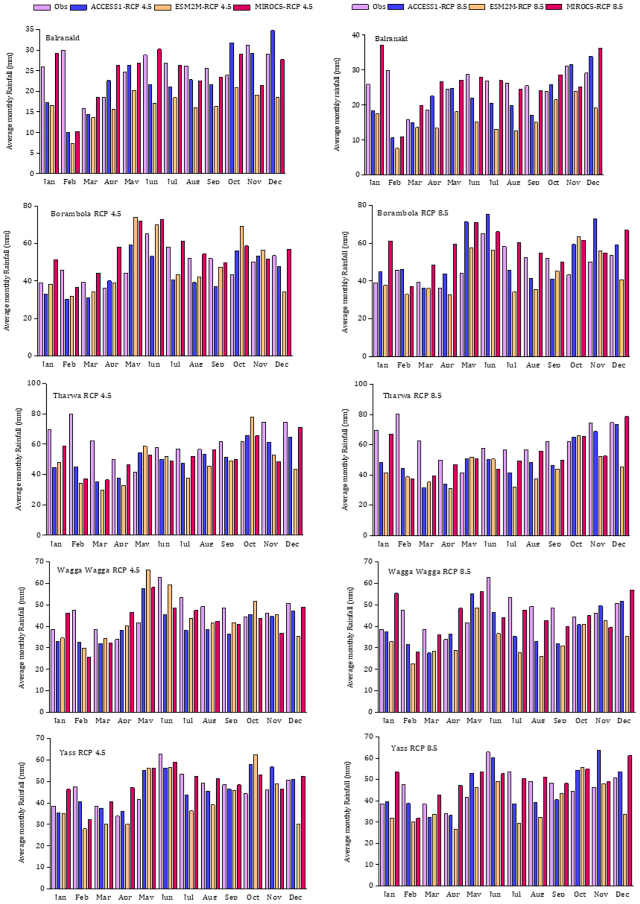
The average annual rainfall of the Murrumbidgee River catchment is about 533 mm (mean annual long-term rainfall data from Balranald, Wagga Wagga, and Yass). This annual rainfall pattern varies from 714 mm to 359 mm between the high elevated area Yass and downstream area Balranald. Most of the rainfall occurs during the winter months (May–October) in Wagga Wagga and Yass, whereas at Balranald, rainfall occurs between June and July. In comparison, long-term average rainfall (1911–2016) with the average record of the last seventeen years (2001–2016) shows autumn rainfall has increased in February by 70% at Balranald (Figure 2a), 51% at Wagga Wagga (Figure 2e), 49% at Yass (Figure 2d), 58% at Borambola (Figure 2b), and 47% at Tharwa (Figure 2c). The rainfall comparison pattern shows a higher trend in Yass and a lower trend downstream of Wagga Wagga (Figure 2e). Thus, total historical summer monthly rainfall is higher in Tharwa and lower in Balranald (Figure 3).

2.2.2. General Circulation Models (GCMs) and Emission Scenarios

General Circulation Models (GCMs) provide global future climate projections of different climate variables. According to the IPCC report, more than forty GCMs have been developed around the world. Among those CMIP5 coarse resolution GCMs, eight GCMs (MIROC5, ACCESS1-0, GFDL-ESM2M, HadGEM2-CC, CESM1-CAM5, NorESM1-M, CNRM-CM5, and CanESM2) have been identified as the best performance model over Australia by the Australian government climate agencies [33]. However, three of these eight models were recommended for representing the “best case”, “worst case”, and “maximum consensus” scenarios for any given region.
These climate models are compatible with future climate scenarios [34]. RCP4.5 is a medium-low stabilization scenario developed by the GCAM modeling team at the Pacific Northwest National Laboratory in the US. It is a stabilization scenario in which radiative forcing stabilizes at 4.5 Wm2 by 2100 with a CO2 concentration of 650 ppm without overshooting the long-run radiative forcing target level [33,34,35,36]. RCP 8.5 is an extremely high greenhouse gas emission scenario, indicating a rising radiative forcing pathway that leads to 8.5 Wm2 by 2100 and a CO2 concentration of 1370 ppm. This RCP was developed by the International Institute for Applied Systems Analysis (IIASA) in Austria using the MESSAGE model and the IIASA Integrated Assessment Framework [34,35].
In this study, the outputs of three GCMs were used to assess the future climate change impact on the Murrumbidgee River basin runoff. MIROC5, GFDL-ESM2M, and ACCESS1.0 are selected to project future climate variables for two representative concentration pathways (RCP 4.5 and RCP 8.5) (Table 2). MIROC5 was chosen as the best-case scenario model for predicting the least increase (or greatest decrease) in evapotranspiration and the greatest increase in precipitation. For the worst-case scenario, the GFDL-ESM2M model was selected, as this model projects the greatest increase in evapotranspiration and the greatest decrease in precipitation. ACCESS1.0 has been used as a maximum consensus scenario model. Maximum consensus is defined as the future climate populated by the greatest number of models, where that number must be at least one-third of the total number of available GCMs and must be at least 10% greater than the next most populous future climate.

2.3. Future Climate Scenario

The following two climate scenarios are employed in this study and have been assessed for future periods, (i) 2016–2035, (ii) 2035–2055, (iii) 2055–2075, and (iv) 2075–2100. These scenarios are defined by daily time series of climate data based on historical rainfall, runoff, and evapotranspiration from 1985 to 2016.
Scenario 1: Representative Concentration Pathway (RCP) 4.5—2016–2035, 2035–2055, 2055–2075, 2075–2100.
Scenario 2: Representative Concentration Pathway (RCP) 8.5—2016–2035, 2035–2055, 2055–2075, 2075–2100.

2.4. Rainfall-Runoff Hydrological Model

The application of a computer-based hydrological model to characterize the water balance and runoff response of the catchment is one of the major paradigms of modern catchment hydrology. A hydrological model is used as a platform for understanding catchment processes by estimating or generating time-series data that may be difficult to measure directly. Following the development of the computing power of the computer, different hydrological models are developed to examine how changes in soil qualities, land use, and climate affect the hydrology and water resources of the watershed [37,38].
SIMHYD is a conceptual rainfall-runoff model, which is developed in Australia to simulate daily stream flow [39]. This rainfall-runoff model is the most widely used, having been applied to over 300 catchments [40,41]. According to a previous study, SIMHYD conceptualizes the runoff from four different sources: direct runoff from impervious areas, runoff due to infiltration excess, interflow, and baseflow from a groundwater store [39]. The model requires daily precipitation and potential evapotranspiration as input data sets to simulate daily runoff and historical stream flow can be used for model calibration and validation. It has the ability to implement multiple runs and an automated calibration technique.
SIMHYD has been used successfully for the estimation of climate change impact on catchment runoff in various regions [20,21,22,23]. In this study, we applied two approaches in order to calibrate the model: (i) the total modeled runoff must be within 5% of the total recorded runoff; and (ii) the ratio of surface runoff to total runoff should be within 20%. The SIMHYD model simulates little to no infiltration excess runoff. Therefore, to optimize the maximum infiltration loss (COEFF), the default value is set to 200, and the infiltration loss exponent (SQ) value is 1.5, which is the recommended value for tropical catchments. The model was calibrated against daily runoff with two constraints and six parameters. [42]. The SIMHYD model is part of Rainfall-Runoff Library (RRL) software which was downloaded from the eWater website [43] and installed on a personal laptop under the free licensing agreement for research purposes. The RRL was configured with the default values available for SIMHYD parameters. These default values specify the initial parameter values as well as boundary limits (Table 3).

2.5. Model Calibration and Validation

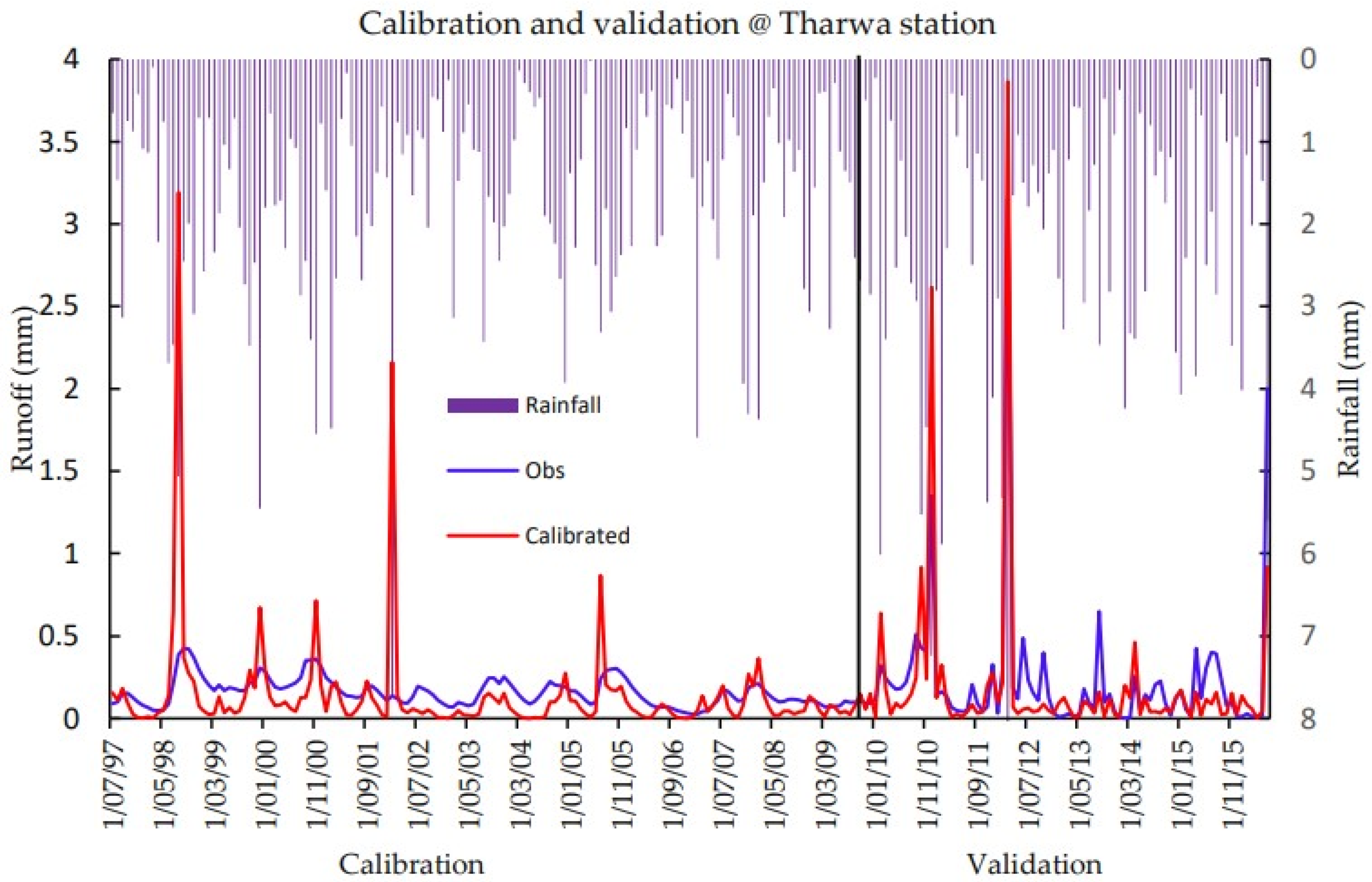
Calibration and validation give a way to assess the robustness of the model. There are different methods of model calibration, and among them, a suitably long period of runoff record is the preferred method. This method helps to verify the model behavior outside the calibration period. It is important to select the calibration and validation periods carefully to cover both wet and dry extremes, and the average annual flow is statistically insignificantly different from the validation period. In this study, the SIMHYD was calibrated against the monthly streamflow data (Figure 4) for a period of fourteen years (1997–2010); two years used for warmup and twelve years for calibration SIMHYD model. Moreover, the model was validated over five years (2012–2017). Both the calibration and validation were done at Balranald station, which is the outlet of the Murrumbidgee River basin. The SIMHYD was calibrated against the daily runoff data for a period of fourteen years (1997–2010), including two years of warmup that covered both extreme wet and dry flows. Moreover, the model was validated with five years of data outside of the calibration period (2012–2017). Both the calibration and validation processes were done at Balranald Station, which is the outlet of the Murrumbidgee River basin. The performance of our hydrological model to simulate the catchment hydrology is measured using the Nash-Sutcliffe Efficiency (NSE) and RMSE [44]. NSE values vary from zero to one. The closer the NSE value is to one, the greater the model’s performance. However, NSE values greater than 0.6 indicate acceptable model performance, and NSE values greater than 0.8 indicate good model performances [24,44,45]. Similarly, an RMSE value near zero shows high model performance.

2.6. Trend Analysis

A non-parametric Mann-Kendall Trend (MK) test is used to examine the presence or absence of monotonic trend time series data of candidate station [46]. The null hypothesis (Ho) of MK is that there is no trend, and the alternative hypothesis (Ha) of MK is that a candidate station’s time series exhibits a monotonic trend over time. Equation (1) is used to calculate the Mann-Kendall test statistic.
S = i = 1 n 1 j = i + 1 n s i g n ( X j X i )  
where Xi and Xj are the sequential data in the series and n is the size of the data series.
Where j > I and i = 1, 2, 3…, n−1 k = 2, 3, 4…, n, and n is the number of data sign (XjXi) is calculated by (Equation (2))
s i g n ( X j X i ) = { + 1   i f ( X j X i ) > 0   0   i f   ( X j X i ) = 0 1   i f   ( X j X i ) < 0
Equation (3) was used to calculate the variance of S
V a r ( S ) = S ( n 1 ) ( 2 n + 5 ) q p t p ( t p 1 ) ( 2 t p + 5 ) 18
where
q is the number of tied groups in the datasets,
tp is the number of data in the pth tied group,
n is the total number of data in the time series.
A positive value of S indicates that an increasing and negative value of S is decreasing trend of time series data of the candidate station. Equation (4) is used to calculate the standardized Mann-Kendall test statistics.
Z s = { S 1 v a r ( S )   i f   S > 0 0   i f   S = 0   S + 1 v a r ( S )   i f   S < 0  
To estimate the magnitude or rate of change the Thiel-Son slope method was used. Equation (5) is used to calculate the Theil–Sen slope (β).
β = m e d i a n ( X j X i j i )  

3. Results

3.1. Model Performance

The SIMHYD model was calibrated and validated using historical streamflow data at three different catchments having gauging stations within the Murrumbidgee River catchment. These catchments were selected for model calibration because of their data consistency for at least 30 years. Consistent and long-term historical data were required to capture the variability in streamflow.
The result shows that the SIMHYD model can generate acceptable observed daily runoff series having NSE model performance values in the range of 0.94 to 0.63 during calibration and validation (Figure 5). The daily flow duration curve (Figure 6) compares the daily modeled and observed runoff for the Murrumbidgee River at Tharwa.

3.2. Spatial and Temporal Variability of Future Rainfall

This section presents the results of rainfall analysis done by comparing historical observed rainfall for the period 1985–2016 with projected rainfall under emission scenarios RCP 4.5 and RCP 8.5 at five different sub-catchments. The analyses were done for annual, monthly, and seasonal changes, respectively, at each station. The analyses show that the ESM2M climate model underestimated the average monthly rainfall in all sub-catchments except for May under both climate scenarios. Applying the same analysis, ACCESS1 underestimated the monthly rainfall over five sub-catchments in the study region during January, February, and March under RCP 4.5 and RCP 8.5 climate scenarios. However, the ACCESS1 climate model overestimated and underestimated the monthly rainfall at five different sub-catchments in the Murrumbidgee River catchment. Exceptionally, for the two climate models, MIROC5 overestimated the monthly rainfall over all sub-catchments in the Murrumbidgee River catchment under both climate scenarios compared to the rainfall in the baseline (historical) (Figure 7).
Likewise, annual and seasonal rainfall over five different sub-catchments were analyzed, and the summarizing result is shown in Figure 8 and Figure 9. Except for Borambola and Yass, all climate models projected that the annual rainfall would decrease over the Balranald, Tharwa, and Wagga Wagga sub-catchments under RCP 4.5 and RCP 8.5 climate scenarios compared to the historical rainfall at each sub-catchment (Figure 8). The summer rainfall is underestimated by all climate models under RCP 4.5 over all sub-catchments. Similarly, all climate models under RCP 8.5 underestimated the summer season rainfall over Balranald sub-catchment. Whereas the autumn, winter, and spring rainfall shows that underestimated over most sub-catchments except for Borambola sub-catchment (Figure 9 and Figure 10) under RCP 4.5 and RCP 8.5 climate scenarios.

3.3. Trend Analysis

A nonparametric Mann-Kendall trend test and Sen’s slope estimator are used to locate the trends and quantify the magnitude of change for future projected rainfall at five different sub-catchments within the Murrumbidgee River catchment. The trend analysis was summarized into baseline, shorter (2016–2045), midterm (2046–2075), and long-term (2075–2104) time spans. Table 4 shows that, except for ESM2M (RCP 8.5), all climate models projected as the winter season rainfall significantly decrease by the value of 0.97–1.59 mm at Balranald catchment. At Borambola catchment, the ACCESS1 climate model projected that the winter season rainfall would decrease significantly by 3.02 mm under RCP 8.5. Similar to Balranald catchment, all climate models project a significant decreasing trend of winter season rainfall at Wagga Wagga catchment under all climate scenarios by 1.69–2.27 mm, except for the ESM2M climate model under the RCP 8.5 scenario. However, for the annual and rest seasons, the rainfall shows decreasing and increasing trends over the selected sub-catchments in the Murrumbidgee River basin for the period 2016–2045 under the RCP 4.5 and RCP 8.5 climate scenarios.

3.4. Rainfall-Runoff Modeling

3.4.1. Baseline Simulation

Future runoff in five sub-catchments of the Murrumbidgee River basin is predicted under RCP 4.5 and RCP 8.5 emission scenarios using the SIMYD conceptual rainfall-runoff model. Figure 11a–e summarizes the modeling results. When compared to historical runoff, all climate models predict a decreasing trend in monthly average runoff at the Tharwa, Yass, and Wagga Wagga sub-catchments (Figure 11a,b,d). However, for the Borambola sub-catchment, the ACCESS1 and MIRCOS models predict the average monthly runoff to increase for the future climate scenario of RCP 4.5 (Figure 11e). However, ESM2M simulated an increasing trend in monthly runoff except for February, March, April, and December for the same sub-catchment. As shown in Figure 11c, all climate models predict increasing and decreasing trends compared to historical runoff over the Balranald sub-catchment. This shows that the runoff generated by each sub-catchment is highly correlated with spatial and temporal rainfall characteristics (Figure 11a–e) for the period of 1985–2016.

3.4.2. Monthly Changes of Future Runoff

In the preceding section, we discussed the spatial and temporal variability of rainfall in the study regions. Furthermore, the trends and their magnitude of change were investigated using the MK test and Sen’s slope estimator for future scenarios under RCP 4.5 and RCP 8.5. Future climate change impacts on stream flow are investigated as follows: Table 5 summarizes monthly runoff change due to climate change in the Murrumbidgee River basin under the emission scenarios RCP-4.5 and RCP-8.5. The results were compared with the average runoff of the historical period of 1985–2016. All climate models simulate future monthly runoff, which will decrease over the sub-catchments. For example, on the Balranald sub-catchment, the average monthly runoff will decrease in the range of 3–95% (Table 5). However, at the Borambola sub-catchment, the ESM2M and MIROC5 climate models underestimate the monthly runoff during December–April and overestimate the monthly runoff during May–November. Conversely, ACCESS1 overestimated monthly futures entirely for the year in the range of 155% to 780%. At the Tharwa sub-catchment, the average monthly runoff would decrease in the range of 8–94% and overestimate the monthly runs of June and October by 6–65%. Likewise, the monthly average runoff at Wagga Wagga and Yass sub-catchments would decrease in the range of 6% to 84% and 1% to 85%, respectively, during most months. Conversely, we overestimated the monthly average runoff by 9% to 97% at Wagga Wagga and 6% to 61% at Yass sub-catchments under the RCP 4.5 climate scenario (Table 5). In general, all climate models predict that future runoff will decrease under the RCP 4.5 climate scenario in five sub-catchments of the Murrumbidgee River basin.
Similarly, for the RCP 8.5 climate scenario, a compression was made at each sub-catchment of the Murrumbidgee River basin, and the result was summarized in Table 6. All climate models simulated the monthly runoff, which would decrease in the range of 13% to 94% and 1.5% to 56% at Balranald and Borambola sub-catchment, respectively (Table 6). But the monthly runoff was overestimated by 11—407% and 14—300%, respectively, over the Balranald and Borambola sub-catchments, respectively. Similarly, the average monthly runoff will decrease in three sub-catchments: Tharwa by 0.2% to 70.9%, Wagga Wagga by 3.8% to 85%, and Yass by 5.7% to 91%. However, during the next few months, there would be an increase in the average monthly runoff over the sub-catchments of the Murrumbidgee River basin (Table 6). In general, all three climate models simulated a decrease in the monthly average runoff over all sub-catchments of the Murrumbidgee River basin during most months under the RCP 4.5 and RCP 8.5 scenarios.

3.4.3. Seasonal Changes of Rainfall and Runoff

The seasonal variation in rainfall and runoff for the entire sub-catchments of the Murrumbidgee River basin were analyzed for the three selected climate models under both RCPs. Each model had varying degrees of capability in terms of simulating seasonal rainfall and runoff under each emission scenario. For example, rainfall in the Balranald sub-catchment will be decreased by 20% to 50% during the summer season and the runoff will be reduced by 37% to 82%. This shows that, for a unit change in future rainfall, the simulated runoff will decrease by nearly twofold over the entire sub-catchments of Murrumbidgee River basin (Table 7). However, for the autumn and winter seasons, the change in future runoff more than doubles for a unit change in rainfall depth under RCP 4.5 (Table 7). Likewise for RCP 8.5 the seasonal rainfall reduced by 1–50% which is resulting to a reduction of the seasonal runoff by 3% to 85% (Table 8). This could be due to a variety of factors, including land use cover change and water abstraction, and would necessitate additional research in addition to climate change.

3.4.4. Annual Changes for RCP 4.5 & RCP 8.5

To look in depth at the impact of climate change, 30 years of rainfall and other climate variables were used and predicted annual runoff change into three-time windows. The percentage change in the mean annual rainfall and runoff compared with the historical rainfall and runoff data are presented in Table 9 and Table 10 for RCP 4.5 and RCP 8.5 emission scenarios. Noteworthy results are that all climate models predicted the future annual rainfall and runoff will decrease overall all sub-catchments of the Murrumbidgee River basin except for MIROC5 at Borambola under RCP 4.5 climate scenario (Table 9). Similarly, all climate models underestimated the future runoff at Balranald, Tharwa, Wagga Wagga, and Yass sub-catchments under RCP 8.5 (Table 10). However, at Borambola sub-catchment ACCESS1, ESM2M climate models are overestimated the annual runoff by 2016–2045 and underestimated the annual runoff by 2046–2075 and 2076–2104 time periods. Conversely, MIROC5 model overestimated the annual runoff at Borambola sub-catchment during the three-time scenarios (Table 10).

3.4.5. Trends of Future Runoff

In the above section, we have calculated average annual rainfall and runoff for three different GCMs applied to each sub-catchment in the Murrumbidgee River catchment. Generally, the climate models show a decrease in annual rainfall in the range of 2% to 72% under RCP 4.5 and 2% to 79% under RCP 8.5, respectively, in the sub-catchments of the Murrumbidgee River catchment. As the results have shown, we have compared the change in annual average runoff by comparing it with historical simulations. Likewise, for the trend analysis for rainfall, the Mann-Kendall trend analysis was applied to check the significance of the change in future runoff for both annual and seasonal changes, and the results were summarized in Table 11. The results in Table 11 that the decreasing trend of annual runoff is statistically significant at Tharwa (simulated by ESM2M and MIROC5) and Wagga Wagga (by MIROC5 sub-catchment) during 2021–2045, respectively, under the RCP 4.5 scenario. There is also a significantly decreasing trend by 2046–2075 and 2076–2104 over the Tharwa sub-catchment in the EMS2M and ACCESS1 climate models under the RCP 4.5 scenario. All climate models simulated a decreasing trend in the annual runoff at the Tharwa and Wagga Wagga sub-catchments during 2016–2045. Moreover, at the Borambola sub-catchment, the annual runoff shows a decreasing trend by the time period of 2016–2045 under the RCP 4.5 scenario (Table 11).

4. Discussion

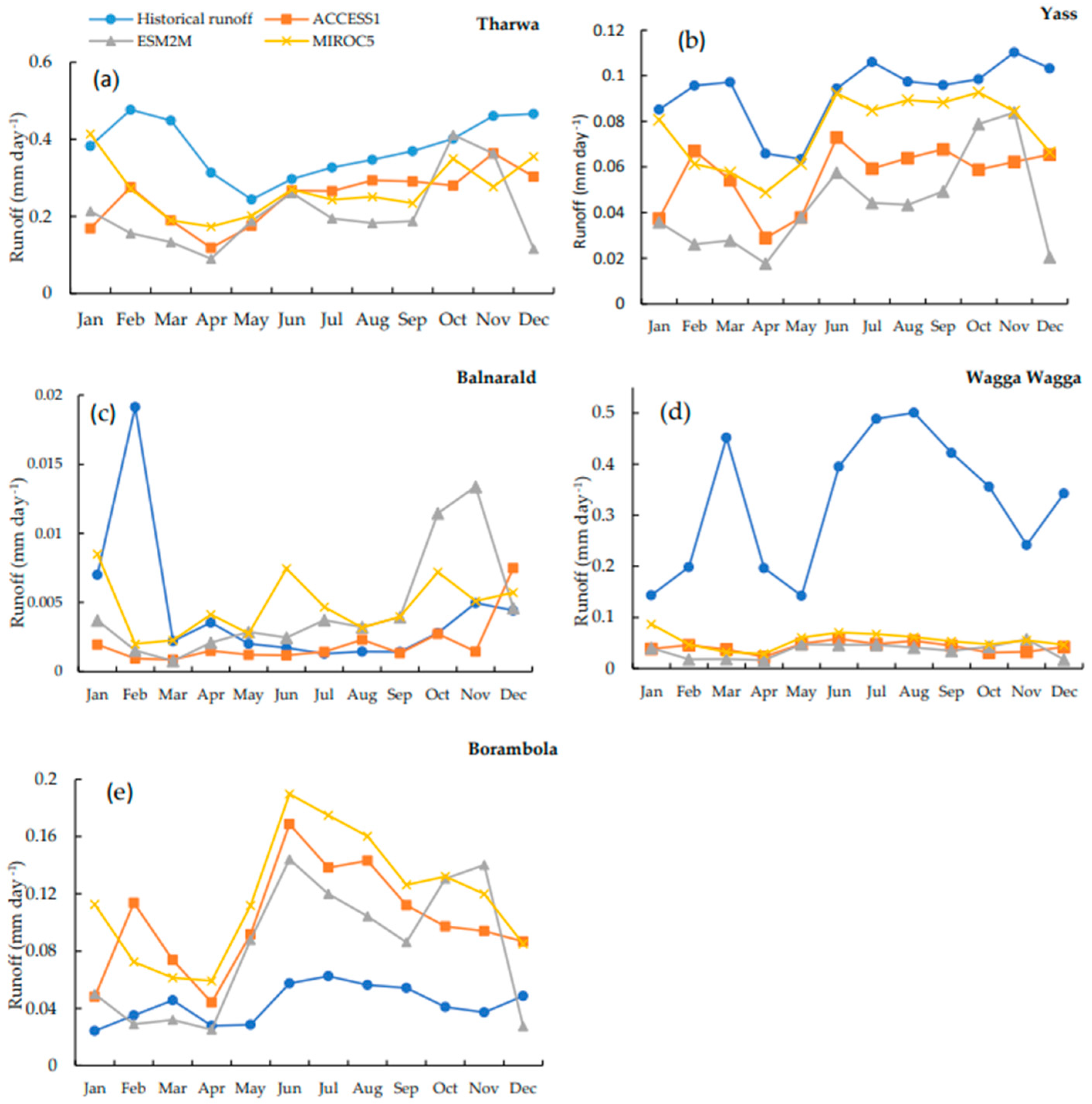
Our study result using three GCMs climate projection showed a decrease in mean annual, and seasonal runoff at Tharwa, Wagga Wagga, and Yass sub-catchments which are similar to a previous study done by Chiew et al. [22]. Study results indicate that potential changes in runoff due to climate change and variability are highly significant. At Tharwa and Yass, the monthly runoff decreasing trend from December to April varies between 6% and 94% for three GCM projected climate data under RCP 4.5 scenario. However, at Borambola the runoff increases from May to November using all GCM projections. Considering seasonal changes at these sub-catchments, the summer runoff decreases by 80% and 82% whereas the winter runoff decreases by 30% and 50%, respectively, using ESM2M projected climate data. However, using ACCESS1 climate projection at Tharwa and Yass sub-catchments, the summer and winter runoff decreases by 67%, 57%, 28%, and 41%, respectively. Moreover, a decreasing trend shows for rest of the model in summer by 52%, 58% and in winter by 12% and 6%, respectively.
Likewise, results also showed a decreasing trend at Wagga Wagga catchment between December and April in the monthly analysis using ACCESS1 and ESM2M model predicted data. The results indicate a possible hydrological drought signal identified at Wagga Wagga sub-catchment area [47]. However, the winter runoff increases by 37% despite rainfall decreasing by 13%. This increased runoff may result of higher rainfall in the neighboring sub-catchment, such as at Borambola, and Yass valley, and additional flow provided by the Snowy Mountains Scheme.
According to Wen et al. [48] the standardized flow index identified considerable increased drying at Balranald, downstream of the Lowbidgee floodplain, particularly after the 1960. It is also important to acknowledge that while this research has considerable simplicity, there are challenges in that many different processes affect river flows, besides climate change, including the clearing of trees, upstream catchment processes, and river regulations. In addition, there are complex climate and storage effects extending over a series of years [48]. Modeling was unlikely to fully capture these processes and effects on the river flow, but the model provided a reasonably good assessment of gross changes in the catchment runoff. Also, this modeling approach is probably not so well equipped to predict future runoff conditions (i.e., data streams were not included). However, increasing current data streams can still be used to model a changing river’s behavior.
The research question and motivation of this research was to find the changes in runoff at various sub-catchments within the Murrumbidgee River basin. All three climate models projected a decreasing rainfall trend in this region under both RCP 4.5 and RCP 8.5 scenarios [49]. Applying GCM predicted future climate data the SIMHYD model also simulates expected runoff for most of the sub-catchments. However, at Borambola sub-catchment, the winter runoff may increase by 366% and 200% using ACCESS1 under both future climate scenarios. This excessive runoff could damage agricultural crops as well as local infrastructure and properties in this region. According to this research, projections of annual and seasonal runoff at the Murrumbidgee region may be accurate, which can be used to improve agriculture and urban development policies.

5. Conclusions

The Murrumbidgee River catchment in the southeast region of the MDB, accounts for 22% of the surface water diversion for irrigation and urban use though it represents only 8% of the total land mass of the MDB. In terms of economy, it contributes 25% of NSW state’s fruit and vegetable production, 42% of the state’s grapes, and half of Australia’s rice production. This agricultural development required setting up an irrigation system by building several dams on the Murrumbidgee River. Moreover, this catchment is highly regulated for hydropower generation upstream by the Snowy Mountains Scheme. These human-induced structures have altered the river’s natural flow dynamics that normally result from external climatic drivers such as precipitation, evapotranspiration, percolation, and runoff.
However, the data on water use, agricultural production, and environmental flows reflect the trends of the history of human settlements, agricultural development, government policy and investment, social issues, and environmental conditions within the Murrumbidgee Catchment. Future climate change-induced alterations in rainfall and evapotranspiration may increase the risks of unexpected drought and flood events. These natural disasters can cause a major impact on the economy, environment, people, and society. In this context, assessing future catchment water availability under predicted future climate alterations is critical for developing effective water management policies and climate change adaptation strategies for catchments.

Author Contributions

Conceptualization, N.M. and G.T.A.; methodology, formal analysis, writing the original draft preparation, S.K.B.; methodology and data analyses, N.M., G.T.A., S.K.B., M.A.J., and E.T.; review and editing, funding acquisition, G.T.A.; funding acquisition. All authors have read and agreed to the published version of the manuscript.

Funding

This research received no external funding. Gebiaw T. Ayele received funding from Griffith Graduate Research School, the Australian Rivers Institute and School of Engineering and Built Environment, Griffith University, Queensland, Australia.

Institutional Review Board Statement

Not applicable as this study was not involved humans or animals.

Informed Consent Statement

Not applicable as there was no human involved.

Data Availability Statement

The data presented in this study are available in the tables and figures presented in the manuscript.

Acknowledgments

This research was supported by the University of Southern Queensland Research Training Program (RTP). This paper is prepared from Newton Muhury’s thesis submitted to fulfill his Master of Science Research degree at USQ. Our sincere thanks to Joachim Ribbe and Shahbaz Mushtaq for their guidance in the preparation of the thesis. Thanks are extended to the Australian Bureau of Meteorology, NSW Office of Water Information, and Climate Change of Australia. Gebiaw T. Ayele acknowledges Griffith Graduate Research School, the Australian Rivers Institute and School of Engineering, Griffith University, Queensland, Australia.

Conflicts of Interest

The authors declare no conflict of interest.

References

  1. Chen, J.; Brissette, F.P.; Lucas-Picher, P.; Caya, D. Impacts of weighting climate models for hydro-meteorological climate change studies. J. Hydrol. 2017, 549, 534–546. [Google Scholar] [CrossRef]
  2. Australian Bureau of Statistics. National Land Account, Experimental Estimates. 2021. Available online: https://abs.gov.au (accessed on 12 July 2022).
  3. IPCC. Climate Change 2014: Synthesis Report. Contribution of Working Groups I, II and III to the Fifth Assessment Report of the Intergovernmental Panel on Climate Change; IPCC: Geneva, Switzerland, 2014; p. 151. Available online: https://epic.awi.de/id/eprint/37530/1 (accessed on 18 July 2022).
  4. Saha, P.P.; Zeleke, K.; Hafeez, M. Streamflow modeling in a fluctuant climate using SWAT: Yass River catchment in southeastern Australia. Environ. Earth Sci. 2014, 71, 5241–5254. [Google Scholar] [CrossRef]
  5. Tan, M.L.; Ibrahim, A.L.; Yusop, Z.; Chua, V.P.; Chan, N.W. Climate change impacts under CMIP5 RCP scenarios on water resources of the Kelantan River Basin, Malaysia. Atmospheric Res. 2017, 189, 1–10. [Google Scholar] [CrossRef]
  6. Turral, H.; Burke, J.; Faurès, J.-M. Climate Change, Water and Food Security; Food and Agriculture Organization of the United Nations (FAO): Rome, Italy, 2011. [Google Scholar]
  7. Climate Change Australia. Australia’s Official Climate Data Projections. Available online: http://www.climatechangeinaustralia.gov.au (accessed on 12 May 2022).
  8. Kingsford, R.; Thomas, R. Use of satellite image analysis to track wetland loss on the Murrumbidgee River floodplain in arid Australia, 1975–1998. Water Sci. Technol. 2002, 45, 45–53. [Google Scholar] [CrossRef] [PubMed]
  9. Kingsford, R.; Thomas, R. Destruction of wetlands and waterbird populations by dams and irrigation on the Murrumbidgee River in arid Australia. Environ. Manag. 2004, 34, 383–396. [Google Scholar] [CrossRef] [PubMed]
  10. Xu, C.-Y. Climate change and hydrologic models: A review of existing gaps and recent research developments. Water Resour. Manag. 1999, 13, 369–382. [Google Scholar] [CrossRef]
  11. Sellami, H.; Benabdallah, S.; La Jeunesse, I.; Vanclooster, M. Quantifying hydrological responses of small Mediterranean catchments under climate change projections. Sci. Total Environ. 2016, 543, 924–936. [Google Scholar] [CrossRef]
  12. Tan, M.L.; Ficklin, D.L.; Ibrahim, A.L.; Yusop, Z. Impacts and uncertainties of climate change on streamflow of the Johor River Basin, Malaysia using a CMIP5 General Circulation Model ensemble. J. Water Clim. Chang. 2014, 5, 676–695. [Google Scholar] [CrossRef]
  13. Park, C.; Min, S.-K.; Lee, D.; Cha, D.-H.; Suh, M.-S.; Kang, H.-S.; Hong, S.-Y.; Lee, D.-K.; Baek, H.-J.; Boo, K.-O.; et al. Evaluation of multiple regional climate models for summer climate extremes over East Asia. Clim. Dyn. 2016, 46, 2469–2486. [Google Scholar] [CrossRef]
  14. Minaei, A.; Todeschini, S.; Sitzenfrei, R.; Creaco, E. Ensemble Evaluation and Member Selection of Regional Climate Models for Impact Models Assessment. Water 2022, 14, 3967. [Google Scholar] [CrossRef]
  15. Zhang, Y.; You, Q.; Chen, C.; Ge, J. Impacts of climate change on streamflows under RCP scenarios: A case study in Xin River Basin, China. Atmospheric Res. 2016, 178, 521–534. [Google Scholar] [CrossRef]
  16. Chiew, F.H. Estimation of rainfall elasticity of streamflow in Australia. Hydrol. Sci. J. 2006, 51, 613–625. [Google Scholar] [CrossRef]
  17. Li, C.; Fang, H. Assessment of climate change impacts on the streamflow for the Mun River in the Mekong Basin, Southeast Asia: Using SWAT model. Catena 2021, 201, 105199. [Google Scholar] [CrossRef]
  18. Zhang, H.; Wang, B.; Liu, D.L.; Leslie, L.M.; Shi, L.; Zhang, M.; Yu, Q. Individual and Coupled Effects of Future Climate and Land Use Scenarios on Water Balance Components in an Australian Catchment. Atmosphere 2022, 13, 1428. [Google Scholar] [CrossRef]
  19. Sankarasubramanian, A.; Vogel, R.M.; Limbrunner, J.F. Climate elasticity of streamflow in the United States. Water Resour. Res. 2001, 37, 1771–1781. [Google Scholar] [CrossRef]
  20. Chiew, F.; McMahon, T. Detection of trend or change in annual flow of Australian rivers. Int. J. Climatol. 2002, 13, 643–653. [Google Scholar] [CrossRef]
  21. Potter, N.; Chiew, F. Statistical characterisation and attribution of recent rainfall and runoff in the Murray-Darling Basin. In Proceedings of the 18th World IMACS Congress and MODSIM09 International Congress on Modelling and Simulation, Modelling and Simulation Society of Australia and New Zealand & International Association for Mathematics and Computers in Simulation, Cairns, Australia, 13–17 July 2009. [Google Scholar]
  22. Chiew, F.; Kirono, D.; Kent, D.; Frost, A.; Charles, S.; Timbal, B.; Nguyen, K.; Fu, G. Comparison of runoff modelled using rainfall from different downscaling methods for historical and future climates. J. Hydrol. 2010, 387, 10–23. [Google Scholar] [CrossRef]
  23. Zhang, Y.; Chiew, F.W. Relative merits of different methods for runoff predictions in ungauged catchments. Water Resour. Res. 2009, 45, W07412. [Google Scholar] [CrossRef]
  24. Peel, M.C.; Chiew, F.H.S.; Western, A.; Mcmahon, T. Extension of unimpaired monthly streamflow data and regionalisation of parameter values to estimate streamflow in ungauged catchments. In National Land and Water Resources Audit; The University of Melbourne: Melbourne, Australia, 2000. [Google Scholar]
  25. Kandasamy, J.; Sounthararajah, D.; Sivabalan, P.; Chanan, A.; Vigneswaran, S.; Sivapalan, M. Socio-hydrologic drivers of the pendulum swing between agricultural development and environmental health: A case study from Murrumbidgee River basin, Australia. Hydrol. Earth Syst. Sci. 2014, 18, 1027–1041. [Google Scholar] [CrossRef]
  26. Norris, R.H.; Liston, P.; Davies, N.; Coysh, J.; Dyer, F.; Linke, S.; Prosser, I.; Young, B. Snapshot of the Murray-Darling Basin River Condition; Murray-Darling Basin Commission: Canberra, Australia, 2001. [Google Scholar]
  27. Wen, L.; Rogers, K.; Saintilan, N.; Ling, J. The influences of climate and hydrology on population dynamics of waterbirds in the lower Murrumbidgee River floodplains in Southeast Australia: Implications for environmental water management. Ecol. Model. 2011, 222, 154–163. [Google Scholar] [CrossRef]
  28. Khan, S.; Akbar, S.; Rana, T.; Abbas, M.A.; Robinson, D.; Paydar, Z.; Dassanayke, D.; Hirsi, I.; Blackwell, J.; Xevi, E.; et al. Off-and-On Farm Savings of Irrigation Water. Murrumbidgee Valley Water Efficiency Feasibility Project; Commonwealth Scientific and Industrial Research Organisation: Canberra, Australia, 2005. [Google Scholar]
  29. Water NSW. NSW Office of Water Information, NSW. 2022. Available online: https://www.water.nsw.gov.au (accessed on 15 April 2022).
  30. Bureau of Meteorology. Australia’s Official Weather Forecasts and Weather Radar. 2017. Available online: http://www.bom.gov.au (accessed on 20 May 2022).
  31. Lee, J.; Kim, S.; Jun, H. A Study of the Influence of the Spatial Distribution of Rain Gauge Networks on Areal Average Rainfall Calculation. Water 2018, 10, 1635. [Google Scholar] [CrossRef]
  32. Barbero, G.; Moisello, U.; Todeschini, S. Evaluation of the Areal Reduction Factor in an Urban Area through Rainfall Records of Limited Length: A Case Study. J. Hydrol. Eng. 2014, 19, 05014016. [Google Scholar] [CrossRef]
  33. Watterson, I.; Abbs, D.; Bhend, J.; Chiew, F.; Church, J.; Ekström, M.; Kirono, D.; Lenton, A.; Lucas, C.; McInnes, K. Rangelands cluster report, climate change in Australia projections for Australia’s natural resource management regions: Cluster reports. In Proceedings of the AMOS National Conference, Brisbane, Australia, 15–17 July 2015. [Google Scholar]
  34. Das, S.K.; Ahsan, A.; Khan, H.R.B.; Tariq, M.A.U.R.; Muttil, N.; Ng, A.W.M. Impacts of Climate Alteration on the Hydrology of the Yarra River Catchment, Australia Using GCMs and SWAT Model. Water 2022, 14, 445. [Google Scholar] [CrossRef]
  35. Van Vuuren, D.P.; Edmonds, J.; Kainuma, M.; Riahi, K.; Thomson, A.; Hibbard, K.; Hurtt, G.C.; Kram, T.; Krey, V.; Lamarque, J.-F.; et al. The representative concentration pathways: An overview. Clim. Change 2011, 109, 5. [Google Scholar] [CrossRef]
  36. Wise, M.; Calvin, K.; Thomson, A.; Clarke, L.; Bond-Lamberty, B.; Sands, R.; Smith, S.J.; Janetos, A.; Edmonds, J. Implications of limiting CO2 concentrations for land use and energy. Science 2009, 324, 1183–1186. [Google Scholar] [CrossRef]
  37. Singh, V.P. Hydrologic modeling: Progress and future directions. Geosci. Lett. 2018, 5, 15. [Google Scholar] [CrossRef]
  38. Wagener, T.; Wheater, H.; Gupta, H. Rainfall-Runoff Modelling in Gauged and Ungauged Catchments; Imperial College Press: London, UK, 2004. [Google Scholar]
  39. Yu, B.; Zhu, Z. A comparative assessment of AWBM and SimHyd for forested watersheds. Hydrol. Sci. J. 2015, 60, 1200–1212. [Google Scholar] [CrossRef]
  40. Chiew, F.H.S.; McMahon, T.A. Modelling the impacts of climate change on Australian streamflow. Hydrol. Process. 2002, 16, 1235–1245. [Google Scholar] [CrossRef]
  41. Chiew, F.H.S.; Peel, M.C.; Western, A.W. Application and Testing of the Simple Rainfall-Runoff Model SIMHYD; Water Resources Publications: Littleton, CO, USA, 2002; pp. 335–367. [Google Scholar]
  42. Chiew, F.; Siriwardena, L. Estimation of SIMHYD parameter values for application in ungauged catchments. In Proceedings of the MODSIM 2005 International Congress on Modelling and Simulation, Melbourne, Australia, 12–15 December 2005; pp. 2883–2889. [Google Scholar]
  43. eWater. Rainfall Runoff Library. Available online: https://ewater.org.au/products/ewater-toolkit/ (accessed on 10 January 2022).
  44. Nash, J.E.; Sutcliffe, J.V. River flow forecasting through conceptual models part I—A discussion of principles. J. Hydrol. 1970, 10, 282–290. [Google Scholar] [CrossRef]
  45. Moriasi, D.; Arnold, J.G.; van Liew, M.W.; Bingner, R.L.; Harmel, R.D.; Veith, T.L. Model Evaluation Guidelines for Systematic Quantification of Accuracy in Watershed Simulations. Trans. ASABE 2007, 50, 885–900. [Google Scholar] [CrossRef]
  46. Kocsis, T.; Kovács-Székely, I.; Anda, A. Homogeneity tests and non-parametric analyses of tendencies in precipitation time series in Keszthely, Western Hungary. Theor. Appl. Climatol. 2020, 139, 849–859. [Google Scholar] [CrossRef]
  47. Leblanc, M.; Tweed, S.; Van Dijk, A.; Timbal, B. A review of historic and future hydrological changes in the Murray-Darling Basin. Glob. Planet. Change 2012, 80–81, 226–246. [Google Scholar] [CrossRef]
  48. Wen, L.; Marsh, V.; Mackay, C.; Salbe, I.; Saintilan, N.; Ling, J. Linking wetland hydrology to ecological outcomes in the Lowbidgee wetlands in Southern New South Wales. In Proceedings of the 19th International Congress on Modelling and Simulation-Sustaining Our Future: Understanding and Living with Uncertainty, MODSIM2011, Perth, Australia, 12–15 December 2011. [Google Scholar]
  49. Van Huijgevoort, M.H.J.; van Lanen, H.; Teuling, A.; Uijlenhoet, R. Identification of changes in hydrological drought characteristics from a multi-GCM driven ensemble constrained by observed discharge. J. Hydrol. 2014, 512, 421–434. [Google Scholar] [CrossRef] [Green Version]
Figure 1. Murrumbidgee River basin study area is located within the Murray Darling Basin in the southeast part of Australia.
Atmosphere 14 00306 g001
Figure 2. Long-term (1911–2016) and short-term (2001–016) historical average rainfall plotted against five different sub-catchments. (a) Long-term and short-term historical average rainfall at Balranald, (b) Long-term and short-term historical average rainfall at Borambola, (c) Long-term and short-term historical average rainfall at Tharwa, (d) Long-term and short-term historical average rainfall at Yass, (e) Long-term and short-term historical average rainfall at Wagga Wagga.
Atmosphere 14 00306 g002
Figure 3. Long-term (1985–2016) historical monthly average rainfall plotted against five different sub-catchments.
Atmosphere 14 00306 g003
Figure 4. SIMHYD model performance criteria during calibration (black squares) and validation (red circles) results at Balranald sub-catchment (mm/day).
Atmosphere 14 00306 g004
Figure 5. The SIMHYD model performance criteria analyzed at Tharwa sub-catchment.
Atmosphere 14 00306 g005
Figure 6. A comparison between observed and SIMHYD modeled runoff during calibration and validation period at Tharwa station.
Atmosphere 14 00306 g006
Figure 7. Predicted and observed monthly average rainfall for sub-catchments in the Murrumbidgee River basin for the period 2016–2035 under the RCP 4.5 climate scenario.
Atmosphere 14 00306 g007
Figure 8. Predicted and observed annual rainfall for sub-catchments in the Murrumbidgee River basin under the RCP 4.5 and RCP 8.5 climate scenarios.
Atmosphere 14 00306 g008
Figure 9. Predicted and observed seasonal rainfall for sub-catchments in the Murrumbidgee River basin under the RCP 4.5 climate scenario.
Atmosphere 14 00306 g009
Figure 10. Predicted and observed seasonal rainfall for sub-catchments in the Murrumbidgee River basin under the RCP 8.5 climate scenario.
Atmosphere 14 00306 g010
Figure 11. The average monthly projected and historical observed runoff trend under the RCP4.5 climate scenario at five different sub-catchments within the Murrumbidgee River catchment. Three GCMs projected future runoff trends under the RCP4.5 climate scenario for period of 2016–2035 plotted against observed historical runoff at five different sub-catchments; a) projected and historical runoff at Tharwa, b) projected and historical runoff at Yass, c) projected and historical runoff at Balranald, d) projected and historical runoff at Wagga Wagga, e) projected and historical runoff at Borambola.
Atmosphere 14 00306 g011
Table 1. The Murrumbidgee River sub-catchment’s location and streamflow gauging station details.
Station IDSite NameLatitudeLongitude
074127Streamflow gauging station at Wagga Wagga−35.12147.37
049002Streamflow gauging station at Balranald−34.63143.57
070108Streamflow gauging station at Yass−34.84148.92
070083Streamflow gauging station at Tharwa−35.51149.06
072155Streamflow gauging station at Borambola−35.17147.63
Table 2. Description of the climate models applied in the study for future climate variable projection under RCP 4.5 and RCP 8.5.
Model NameGroupCountryAtmospheric Resolution
(Longitude × Latitude)
Australian Community Climate and Earth System Simulator (ACCESS1.0)ACCESS1.0Australia1.25 × 1.875
NOAA Geophysical Fluid Dynamics Laboratory−Earth System ModelGFDL-ESM2MUSA2.0225 × 2.5
Model for Interdisciplinary Research on ClimateMIROC5Japan1.4008 × 1.40625
Table 3. The default parameters applied in the SIMHYD modeling with their boundary values.
Name of the ParameterUnitModeled ValueMinimumMaximum
Baseflow Coefficient 0.0940.01.0
Impervious Thresholdmm0.05505
Infiltration Coefficient 92.20400
Infiltration Shape 1.22010
Interflow Coefficient 0.940.01.0
Pervious faction 0.940.01.0
Rainfall Interception Store Capacitymm1.50.05.0
Recharge Coefficient 0.20.01.0
Soil Moisture Store Capacitymm4551500
Table 4. Seasonal and Annual trends of rainfall at five stations for the period of 2016–2045 under all climate models and RCPs.
StationsModelScenariosAnnualSummerAutumnWinterSpring
ZsβZsβZsβZsβZsβ
BalranaldObservedBaseline
ACCESS1RCP 4.50.48−1.190.970.040.800.220.04 *−1.150.241.04
ACCESS1RCP 8.50.48−1.750.670.371.00−0.020.05 *−1.020.231.39
ESM2MRCP 4.50.91−0.220.350.480.500.290.05 *−0.970.120.75
ESM2MRCP 8.50.67−0.680.570.460.390.590.06−1.080.520.67
MIROC5RCP 4.50.78−0.980.640.400.450.510.03 *−1.440.270.81
MIROC5RCP 8.50.91−0.480.410.910.390.500.03 *−1.590.210.92
BorambolaObservedBaseline
ACCESS1RCP 4.50.80−0.510.520.610.750.190.23-0.630.081.26
ACCESS1RCP 8.50.32−3.880.86−0.340.45−0.900.04 *−3.020.83−0.82
ESM2MRCP 4.50.19−3.430.97−0.010.83−0.230.09−2.350.57−1.47
ESM2MRCP 8.50.11−6.540.72−0.390.80−0.510.05−3.620.50−2.05
MIROC5RCP 4.50.13−3.680.80−0.450.69−0.980.07−2.830.57−1.28
MIROC5RCP 8.50.11−4.890.890.170.59−1.090.09−2.890.48−1.11
TharwaObservedBaseline
ACCESS1RCP 4.50.34−2.940.69−0.450.64−0.650.28−1.580.970.25
ACCESS1RCP 8.50.13−4.430.25−2.210.32−1.820.11−2.071.00−0.01
ESM2MRCP 4.50.07−5.620.30−1.360.52−0.830.07−2.320.50−1.36
ESM2MRCP 8.50.03 *−6.480.16−2.160.48−1.310.21−2.320.50−1.83
MIROC5RCP 4.50.02 *−6.660.27−2.470.27−1.930.09−2.350.43−1.13
MIROC5RCP 8.50.02 *−6.140.37−1.920.27−1.840.10−2.410.52−0.79
Wagga WaggaObservedBaseline
ACCESS1RCP 4.50.07−5.210.12−1.810.54−0.710.03 *−2.260.72−0.57
ACCESS1RCP 8.50.09−4.480.12−1.380.34−1.010.05 *−1.960.83−0.28
ESM2MRCP 4.50.39−2.310.59−0.520.62−0.520.16−1.690.62−0.44
ESM2MRCP 8.50.09−4.790.20−1.270.64−0.410.04 *−2.300.45−0.91
MIROC5RCP 4.50.12−4.790.32−1.400.54−0.520.04 *−2.050.62−0.58
MIROC5RCP 8.50.12−4.780.52−0.720.64−0.360.03 *−2.270.59−0.68
YassObservedBaseline
ACCESS1RCP 4.50.13−4.250.35−1.280.57−0.790.10−2.510.75−0.58
ACCESS1RCP 8.50.34−2.460.48-0.840.41−0.930.16−1.860.80−0.43
ESM2MRCP 4.50.34−2.600.83−0.201.00−0.050.10−2.170.62−1.40
ESM2MRCP 8.50.10−5.540.43−0.680.64−0.590.08−2.280.52−1.61
MIROC5RCP 4.50.09−5.170.69−0.580.59−1.260.09−2.260.64−1.12
MIROC5RCP 8.50.09−4.480.64−0.610.34−1.350.13−1.950.75−0.62
* Significance at a 95% confidence level with the corresponding critical value of 1.96 and bold shows the magnitude of change.
Table 5. Change (%) of runoff between simulated (using future climate data) compared to the historical for RCP 4.5 at sub-catchments of Murrumbidgee River basin.
SubcatchmentModelsJanFebMarAprMayJunJulAugSepOctNovDec
BalranaldACCESS1−68−92−74−17−27−29−26−7−329−15−15
ESM2M−72−95−74−51−60−63−43−39−24−42−61−73
MIROC555−91−6117−2536441012−3−57−54
BorambolaACCESS1706155202562711488217436263780650696
ESM2M−21−66−72−4798260386443293103−71
MIROC5135−35−563712533826537013123035−17
TharwaACCESS1−61−71−91−90−86−32−39−2013−22−66
ESM2M−58−84−94−93−364−46−60−4765−29−85
MIROC5−6−72−90−85−2126−20−22−2821−52−54
Wagga WaggaACCESS1−15−63−79−3531−45−72−54−61−2643−56
ESM2M−34−73−81−435597−63657129−66
MIROC577−74−84−2217−39−52−25−31−37−45−57
YassACCESS1−56−39−73−85−1823−57−54−29619−68
ESM2M−69−73−74−91−52−11−76−81−54−19−34−85
MIROC5−20−64−82−73−1330−21−6−16−50−70
Table 6. Change (%) of runoff between simulated (using future climate data) compared to the historical for RCP 8.5 at the sub-catchments of Murrumbidgee River basin.
SubcatchmentModelsJanFebMarAprMayJunJulAugSepOctNovDec
BalranaldACCESS1−61−90−73−13−39−30.3−27−21.927−35.3−21−13
ESM2M−68−94−73−60−67−68.7−65−60.8−40−47.4−38−69.7
MIROC5407−87−5413−2211.34723.427−7.84−45−17.6
BorambolaACCESS16039−61−261304387599.920179188−2.55
ESM2M−22−56−41−561778.3−7−1.561490.579−54.1
MIROC5300−12−40591582311993191322754777.2
TharwaACCESS1−49−71−92−92−4135−40−56.3−45−1.62−22−25.8
ESM2M−59−64−83−93−4060.4−63−70.9−60−17−31−83.1
MIROC5132−8.5−170.419−29−7.43.23−0.262.96.854.1
Wagga WaggaACCESS134−63−85−5025−37.5−74−61.9−65−58.3−7.3−46.6
ESM2M−19−81−85−68−31−73.1−85−80.6−74−59.2−20−72.9
MIROC5247−46−80−3.919−54.2−55−35.4−39−18.7−40−34.4
YassACCESS1−46−59−86−87−3371.6−55−61.7−4922.4−5.7−60.6
ESM2M−69−73−74−91−52−10.6−76−81.2−54−19.2−34−84.9
MIROC524−66−80−73−19−12.4−41−33.2−2217.9−44−50.2
Table 7. Seasonal change (%) of rainfall and runoff for RCP 4.5 at sub-catchments of Murrumbidgee River basin.
SubcatchmentModelsSummerAutumnWinterSpring
RainfallRunoffRainfallRunoffRainfallRunoffRainfallRunoff
BalranaldACCESS1−28−627−42−20−2233
ESM2M−50−82−16−63−37−50−30−47
MIROC5−21−3722−28−331−8−23
BorambolaACCESS1−204879435−243661534
ESM2M−25−6023−16−1111719138
MIROC5424519731810135
TharwaACCESS1−31−67−17−80−12−28−10−9
ESM2M−44−80−21−82−21−30−9−4
MIROC5−26−52−12−79−8−12−17−19
Wagga WaggaACCESS1−18−5212−39−26−59−9−24
ESM2M−27−6324−35−1337031
MIROC5−12−4120−43−16−41−13−36
YassACCESS1−8−5713−68−12−41168
ESM2M−32−822−80−20−5013−9
MIROC5−5−5826−66−1−66−10
Table 8. Seasonal change (%) of rainfall and simulated runoff for RCP 8.5 at sub-catchments of Murrumbidgee River basin.
SubcatchmentModelsSummerAutumnWinterSpring
RainfallRunoffRainfallRunoffRainfallRunoffRainfallRunoff
BalranaldACCESS1−27−596−45−24−27−7−28
ESM2M−48−79−24−67−50−65−25−42
MIROC5−17925−25−326−3−17
BorambolaACCESS1824264−820019117
ESM2M−20−496−27−28221356
MIROC519824941324414152
TharwaACCESS1−27−46−24−85−18−31−9−24
ESM2M−44−73−23−81−30−42−18−37
MIROC5−19−24−11−78−13−36−16−25
Wagga WaggaACCESS1−12−405−46−31−59−12−49
ESM2M−34−67−7−66−46−80−18−56
MIROC521023−37−19−50−10−33
YassACCESS1−4−584−77−17−3514−17
ESM2M−31−78−7−76−33−676−38
MIROC56−4126−67−7−3210−15
Table 9. Annual change (%) of runoff between simulated (using future climate data) compared to the historical for RCP 4.5 at sub-catchments of Murrumbidgee River basin.
SubcatchmentModels2016–20452046–20752076–2104
RainfallRunoffRainfallRunoffRainfallRunoff
BalranaldACCESS1−16−48−9−30−7−31
ESM2M−41−72−35−65−28−57
MIROC5−8−2830−9−32
BorambolaACCESS1−62961222219123
ESM2M−142286−152
MIROC5161371921510117
TharwaACCESS1−16−50−15−44−23−57
ESM2M−25−58−24−51−25−51
MIROC5−13−39−15−37−21−56
Wagga
Wagga
ACCESS1−17−60−6−33−13−49
ESM2M−23−64−6201362
MIROC5−9−45−3−29−9−47
YassACCESS1−2−548−25−3−42
ESM2M−11−63−8−45−11−55
MIROC512−176−25−2−47
Table 10. Annual change (%) of runoff between simulated (using future climate data) comparing to the historical for RCP 8.5 at sub-catchments of Murrumbidgee River basin.
SubcatchmentModels2016–20452046–20752076–2104
RainfallRunoffRainfallRunoffRainfallRunoff
BalranaldACCESS1−6−32−14−44−24−54
ESM2M−23−52−39−68−53−79
MIROC5−8−223241485
BorambolaACCESS1117819234−29
ESM2M884−10−18−24−53
MIROC510871513233237
TharwaACCESS1−19−58−15−30−25−63
ESM2M−19−42−30−60−41−81
MIROC5−20−55−19−53−6−25
Wagga
Wagga
ACCESS1−11−50−8−36−24−70
ESM2M−15−57−28−73−41−82
MIROC5−12−50−6−489−4
YassACCESS1−2−617−10−10−65
ESM2M−3−46−18−67−32−83
MIROC5−2−586−3518−23
Table 11. Trend analysis of annual runoff at sub-catchments of Murrumbidgee River basin under RCP 4.5 and RCP 8.5 scenarios.
RCP 4.5RCP 8.5
SubcatchmentsModel2016–20452046–20752076–21042016–20452046–20752076–2104
ZsβZsβZsβZsβZsβZsβ
BalranaldACCESS10.39−0.020.910.000.840.010.39−0.030.75−0.010.990.00
ESM2M0.62−0.010.08−0.020.960.000.72−0.010.28−0.010.870.00
MIROC50.39−0.031.000.000.81−0.010.50−0.030.540.020.930.00
BorambolaACCESS10.80−0.510.570.390.28−0.720.24−0.760.57−0.350.32−0.29
ESM2M0.09−0.630.43−0.350.27−0.520.04 *−1.160.91−0.040.20−0.15
MIROC50.12−1.030.800.150.34−0.590.03 *−1.140.540.370.21−1.44
TharwaACCESS10.06−0.580.780.110.10−0.410.04 *−0.520.15−0.400.21−0.22
ESM2M0.03 *−0.600.11−0.410.24−0.400.02 *−0.890.62−0.110.12−0.16
MIROC50.01 *−0.990.890.100.09−0.490.01 *−0.740.910.050.42−0.39
Wagga WaggaACCESS10.00 *−0.340.910.020.04 *−0.320.00 *−0.410.18−0.200.05 *−0.19
ESM2M0.07−0.210.02 *−0.540.21−0.780.01 *−0.330.28−0.060.10−0.07
MIROC50.00 *−0.440.50−0.110.05−0.370.01 *−0.350.94−0.010.07−0.48
YassACCESS10.09−0.350.940.030.44−0.260.34−0.220.41−0.220.32−0.14
ESM2M0.30−0.210.35−0.190.30−0.190.12−0.310.89−0.020.27−0.09
MIROC50.09−0.690.890.080.38−0.260.11−0.340.480.260.46−0.36
Zs is Mann-Kendall test statistics and β is Son’s slope estimator (magnitude of change). * Significance at a 95% confidence level with the corresponding critical value of 1.96 and bold shows the magnitude of change.
Disclaimer/Publisher’s Note: The statements, opinions and data contained in all publications are solely those of the individual author(s) and contributor(s) and not of MDPI and/or the editor(s). MDPI and/or the editor(s) disclaim responsibility for any injury to people or property resulting from any ideas, methods, instructions or products referred to in the content.

