Abstract
Atmospheric water vapor is an essential source of information that predicts global climate change, rainfall, and disaster-natured weather. It is also a vital source of error for Earth observation systems, such as the global navigation satellite system (GNSS). The Zenith Tropospheric Delay (ZTD) plays a crucial role in applications, such as atmospheric water vapor inversion and GNSS precision positioning. ZTD has specific temporal and spatial variation characteristics. Real-time ZTD modeling is widely used in modern society. The conventional back propagation (BP) neural network model has issues, such as local, optimal, and long short-term memory (LSTM) model needs, which help by relying on long historical data. A regional/single station ZTD combination prediction model with high precision, efficiency, and suitability for online modeling was proposed. The model, called K-RBF, is based on the machine learning algorithms of radial basis function (RBF) neural network, assisted by the K-means cluster algorithm (K-RBF) and LSTM of real-time parameter updating (R-LSTM). An online updating mechanism is adopted to improve the modeling efficiency of the traditional LSTM. Taking the ZTD data (5 min sampling interval) of 13 international GNSS service stations in southern California in the United States for 90 consecutive days, K-RBF, R-LSTM, and K-RBF were used for regions, single stations, and a combination of ZTD prediction models regarding research, respectively. Real-time/near real-time prediction results show that the root-mean-square error (RMSE), mean absolute error (MAE), coefficient of determination (R2), and training time consumption (TTC) of the K-RBF model with 13 station data are 8.35 mm, 6.89 mm, 0.61, and 4.78 s, respectively. The accuracy and efficiency of the K-RBF model are improved compared with those of the conventional BP model. The RMSE, MAE, R2, and TTC of the R-LSTM model with WHC1 station data are 6.74 mm, 5.92 mm, 0.98, and 0.18 s, which improved by 67.43%, 66.42%, 63.33%, and 97.70% compared with those of the LSTM model. The comparison experiments of different historical observation data in 24 groups show that the real-time update model has strong applicability and accuracy for the time prediction of small sample data. The RMSE and MAE of K-RBF with 13 station data are 4.37 mm and 3.64 mm, which improved by 47.70% and 47.20% compared to K-RBF and by 28.48% and 31.29% compared to R-LSTM, respectively. The changes in the temporospatial features of ZTD are considered, as well, in the combination model.
1. Introduction
1.1. Motivations
Climate change and extreme weather are major threats to the sustainability of our society. As an important greenhouse gas, atmospheric water vapor plays a very important role in climate change research and weather forecasting, especially in extreme weather nowcasting [1,2]. The presence of water vapor can lead to tens of meter range measurement errors. Therefore, it is also an important source of error for earth observation systems, such as the Global Navigation Satellite System (GNSS) [3]. It also plays a crucial role in the global water cycle. The water vapor on the Earth mainly comes from the evaporation of the ocean’s surface. The atmospheric flows transport the evaporated water vapor over the continent to form precipitation and then return to the ocean through rivers and underground runoff, thereby forming the atmospheric terrestrial marine water cycle [4,5,6]. Carbon, nitrogen, and water cycles in terrestrial ecosystems are connected and coupled with one another, jointly driving the key processes of the balance of carbon revenue and expenditure in the ecosystem [7]. Global climate change, rising atmospheric CO2 concentration, increased deposition of atmospheric nitrogen, and changes in precipitation patterns affect the carbon revenue and expenditure balance and carbon exchange capacity of terrestrial ecosystems at various levels. However, as of now, the key processes of carbon–nitrogen–water coupling cycles and biological regulation mechanisms in terrestrial ecosystems must be strengthened to evaluate the carbon exchange function and spatial pattern of terrestrial ecosystems and their response and feedback to global changes in land ecosystems accurately. Therefore, exploring carbon–nitrogen–water coupling cycles in terrestrial ecosystems and their responses and adaptation mechanisms to climate change is urgent [8]. It can provide a scientific basis for the carbon–nitrogen–water coupling research in terrestrial ecosystems, increase carbon sinks, and reduce pollution emissions, thereby helping China achieve its “double carbon” goals.
Zenith tropospheric delay (ZTD) can be divided into zenith hydrostatic delay (ZHD) and zenith non-hydrostatic delay, which is always called zenith wet delay (ZWD) [9]. ZWD can be converted into precipitable water vapor, PWV. It is an important factor that affects GNSS navigation and positioning accuracy. In recent years, with the gradual improvement of the high spatiotemporal resolution of ZTD products and the more frequent occurrences of disastrous weather conditions, such as thunderstorms and typhoons, regional real-time/near real-time ZTD modeling has gradually become a hot issue in GNSS and other research fields [10]. This research has important research significance and economic benefits [11].
According to the different conditions of ZTD model application (mainly referring to whether meteorological parameters are needed), the ZTD model can be divided into two categories. The first kind of ZTD model needs measured meteorological parameters (e.g., atmospheric pressure, water vapor pressure, and temperature), which mainly include Hopfield, Saastamoinen, and Black models [12]. In the actual navigation and positioning, meteorological parameters cannot be obtained sometimes, or the obtained meteorological parameters are unstable, thereby causing inconvenience for navigation and positioning. Given this problem, many scholars have established a second type of empirical ZTD model without the use of measured meteorological parameters, which only relies on a large number of empirical data to establish the mapping among various influencing factors and ZTD. Considering that the participation of any meteorological parameters is not needed, the empirical ZTD model, which mainly includes the early UNB series and EGNOS models, as well as GPT2, GPT2w, and IGGtrop models proposed by some scholars in recent years, has made great progress [13].
In recent years, with the rapid development of numerical weather prediction (NWP) and the encryption of GNSS observation stations in the region, empirical models that are more suitable for a certain region are established by fusing the multi-source observation data using spatiotemporal analysis methods. Usually, the long-term linear trend of ZTD is obtained by least-squares [14] and maximum likelihood estimation. The nonlinear characteristics of ZTD (e.g., trend features, short-period disturbances [15], and seasonal periodicities) are obtained by time series analysis methods, such as wavelet analysis [16], spectral analysis, and intelligent analysis. The relationship between ZTD and topography, station elevation, latitude, and longitude is analyzed by spatial structure function, iterative tropospheric decomposition, seasonal Gaussian function, and least-squares collocation methods [17]. For the alpine area of Switzerland, Wilgan and Geiger [18] presented high-resolution models of tropospheric total refractivity and ZTD. Different combinations of data sources, including NWP and GNSS data, were used in the models. Using least-squares collocation, the tropospheric parameters were interpolated to arbitrary locations. Chen et al. [19] analyzed the temporal and spatial characteristics of the ZTD data of GNSS stations of the Crustal Movement Observation Network of China (CMONOC), which was measured for six years. They also established the ZTD empirical model (SHAtrop) for mainland China by using the periodic and grid functions. The accuracy was better than the common empirical models (such as EGNOS, UNB3 m, and GPT2). Zhao et al. [20] established the high-precision ZTD model of altitude-related correction with China as the research area. The ZTD residuals were obtained based on the ZTD initial values determined by the GPT3 model and the GNSS-derived ZTD values. The annual, semi-annual, and seasonal cycles of the residual were analyzed. Moreover, the relationship between the residual and GNSS elevation was analyzed. To some extent, the model overcame the defect, in which the existing empirical ZTD model failed to consider the influence of height on ZTD well.
Owing to the spatial inhomogeneity and temporal variability of atmospheric density and the nonlinear relationship among different meteorological parameters [21], ZTD has the characteristics of dynamic variability, many influencing factors, and strong randomness. Studying the physical mechanism of ZTD [22,23] is difficult, especially for ZTD’s high spatial and temporal resolution modeling in areas with rugged terrain and large meteorological contrast [17]. Without explicitly providing the physical mechanism, data-driven models that use machine learning (ML) approaches have become a hot research topic. The main tasks of ML include supervised learning (e.g., classification and regression), unsupervised learning (e.g., clustering and dimensionality reduction), and reinforcement learning (e.g., control and decision-making), which can deal with nonlinear problems better and are widely used in data interpolation, modeling, and forecasting. In recent years, ML technology has been widely used in several fields and has achieved certain achievements in ZTD modeling. Such models include multi-layer perceptron, adaptive network-based fuzzy inference system (ANFIS), artificial neural network (ANN), and least-squares support vector machine (LSSVM) [24]. The most widely used model is the regional tropospheric model, based on ANN, which realizes the interpolation, prediction, fusion, or improvement of tropospheric delay correction parameters by inputting different parameters in global or local areas. Taking the ZTD data of global positioning system (GPS) stations in the Southern California GPS network as the research object, Wang et al. [25] investigated the ZTD prediction model by using the backpropagation (BP) neural network algorithm and by taking the longitude, latitude, and altitude of the station as inputs. To overcome a large amount of computing volume, proneness to the “over-fitting” phenomenon, and the problem of model instability of the traditional BP neural network, Xiao et al. proposed an improved BP neural network to establish a regional ZTD model. The model takes the normalized geodetic longitude, latitude, and geodetic height as the model inputs, as well as ZTD as the output [26]. Based on the ZTD data of North America, Li conducted ZTD modeling using the BP neural network, LSSVM, and radial basis function (RBF) neural network and systematically evaluated the modeling accuracy, efficiency, and stability of different models. The results show that the RFB algorithm has the best effect in small-scale sample modeling, and the BP algorithm has evident advantages in large-scale sample modeling [27]. Shi et al. proposed a long short-term memory (LSTM) network ZTD prediction model based on Keras platform and compared it with the prediction effects of the BP neural network model. The experimental results show that the root mean square error (RMSE) of the prediction results of the LSTM model reaches the mm level, and its mean absolute error (MAE) and mean absolute percentage error (MAPE) are lower than those of the BP model. The accuracy and stability of the LSTM model are significantly improved compared with those of the BP model [28]. With the comprehensive consideration of the spatiotemporal information of the GPS stations in West Antarctica, Zhang et al. conducted ZTD modeling through two blind source separation algorithms, namely, principal component analysis (PCA), independent component analysis (ICA), and BP neural network and performed high-precision ZTD prediction using the LSTM network [29]. Li et al. improved the ZTD correction performance of the GPT3 model in Antarctica using RBF and LSTM models in terms of space and time, respectively [30]. Zhang et al. proposed a new ZTD time-series forecasting method that used transformer-based machine-learning techniques [31]. For the investigation, analysis, and forecasting of ZTD, the global VMF stations provided by the global geodetic observing system (GGOS) during 2008–2020 were used. Results showed that forecasted ZTD results were more accurate than those of LSTM, RNN, convolutional neural network (CNN), and GPT3 series models. Zhang et al. [22] estimated the ZTD of seven GNSS monitoring stations in China for two consecutive years by using static precise point positioning (PPP) technology. The K-nearest neighbor (KNN) algorithm was used to interpolate the ZTD data gap. The ZTD difference values between KNN and periodic models were trained and predicted by LSTM. The predicted value, combined with the periodic model (ZTD), restored the final ZTD prediction result (LSTM-ZTD), which was better than BP neural network modeling. Static PPP verification experiments with the LSTM-ZTD showed that PPP convergence time was improved in summer, autumn, and winter compared with GPT2 ZTD. Shamshiri et al. [17] developed a new method based on ML Gaussian process (GP) regression approach using the combination of small-baseline interferograms and GNSS-derived ZTD values to mitigate phase delay caused by the troposphere in interferometric observations. On average, it reduced RMSE by 83%, compared to 50%, by using ERA-Interim to correct tropospheric data. Zheng et al. [32] developed a stacked ML model for mapping ZTD into PWV without meteorological parameters. The fifth-generation European Center for Medium-range Weather Forecast Reanalysis (ERA5) and radiosonde information were used to assess and validate the model’s performance. The proposed model performed better than the physical model that used GPT3-derived meteorological parameters. Other techniques that can sense ZTD can benefit from this model for real-time PWV retrieval. Chkeir et al. [21] studied nowcasting extreme rain and extreme wind speed with 3 ML techniques, namely, ANN, LSTM, and LSTM Encoder Decoder (LSTM E/D), applied to different input datasets from ground-based weather sensors, GNSS receivers, C-band radars, and lightning detectors. The analysis showed that the LSTM E/D approach was suitable for the nowcasting of meteorological variables.
1.2. Contributions
Most of the aforementioned ML models focus on BP neural network and LSTM. BP neural network refers to an adaptive nonlinear dynamic system with strong learning and memory functions. However, it has the disadvantage of slow convergence speed and easily falls into local optimum. LSTM can remember long and short-term information and solves the problem of gradient disappearance and explosion during long sequence training; however, it cannot be parallelized and is time consuming [31]. The shortcomings of the two models limit their application ability in real-time high-precision regional ZTD modeling. With the continuous development of real-time precision positioning technologies (e.g., real-time kinematic positioning (RTK), regional continuously-operating reference station (CORS), real-time PPP (RT-PPP), and integer ambiguity resolution-enabled precise point positioning (PPP-RTK)) and the frequent occurrence of extreme weather, the use of the ZTD spatiotemporal information of regional GNSS monitoring stations for regional real-time ZTD high-precision modeling has become a key technology for real-time precision positioning and short-term strong convective weather forecasting. The model will exhibit high precision, spatiotemporal resolution, reliability, and timeliness. It can collect the current ZTD data of some regional GNSS monitoring stations to carry out ZTD spatiotemporal modeling, provide regional atmospheric enhancement products for real-time precise positioning, offer short-term and imminent forecasting services for strong convective disaster weather for seconds to hours, and support data bases for the study of mutual conversion processes, such as condensation and evaporation of water vapor [33]. RBF has the characteristics of high stability, fast convergence speed, and global approximation, and LSTM has been widely used in ZTD modeling and short-term weather forecast. However, its algorithmic effectiveness and optimization research in regional real-time ZTD modeling applications are unsatisfactory. This paper attempts to improve them from the aspects of modeling efficiency and modeling accuracy.
1.3. Organization
Overall, the proposal of a high-precision ZTD model based on ML algorithms suitable for online modeling is expected, and the model accuracy is not affected by factors, such as elevation. The remainder of the paper is summarized as follows. Section 2 uses the ZTD data (5 min sampling interval) of 13 international GNSS service (IGS) stations in southern California in the United States for 90 consecutive days. Given that the real-time meteorological parameters do not need to be inputted based on the three-dimensional coordinates and time of the participating modeling stations as input, the RBF neural network assisted by the K-means cluster algorithm (K-RBF) is used to construct a regional ZTD prediction model. In addition, based on the single station ZTD non-full life cycle historical time series data (few epochs), the single station ZTD prediction model is established by using the LSTM of real-time parameter updating (R-LSTM). Finally, based on the two ZTD models, a regional/single-station ZTD prediction model combined with K-RBF and R-LSTM (KR-RBF-LSTM) is proposed. Section 3 presents the modeling results of the three different ZTD models. Section 4 discusses the modeling effect in terms of modeling efficiency and accuracy. Section 5 presents the conclusion and mentions the limitations of this work and future research direction.
2. Materials and Methods
2.1. Study Region and Datasets
The final ZTD data of 13 IGS monitoring stations in southern California are selected (ftp://igs.gnsswhu.cn/pub/gps/products/troposphere/new, accessed on 11 December 2022). The plane position of the station and its elevation distribution are shown in Figure 1 and Figure 2, respectively. The data period is 90 days, that is, from 12 June 2021 to 9 September 2021. The day of the year (DOY) is from 163 to 252. The sampling interval is 5 min. The final ZTD data are used to simulate ZTD real-time or near real-time modeling. In K-RBF modeling, in t epoch, the data of 12 stations are used for modeling, and the remaining station data are used for accuracy verification. For R-LSTM modeling, for a station on the i-th day, when the epoch t = 6, the data of the first five epochs at the day are used for modeling, and the data of the current epoch t are used for accuracy verification. When t > 6, the data of epoch t-1 are used for modeling, and the data of the current epoch t are used for accuracy verification. KR-RBF-LSTM modeling is performed on the basis of the two aforementioned modeling methods. The modeling results of the first five epochs of each day are removed to compare the accuracy of different models. For 1 of the 13 stations, 283 epoch predicted data are involved in the statistical analysis of the model accuracy in a day, and 25,470 epochs are involved in the accuracy statistics for 90 consecutive days.
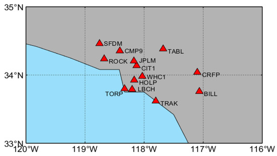
Figure 1.
IGS monitoring station distribution map. Note: The station names are BILL, CIT1, CMP9, CRFP, HOLP, JPLM, LBCH, ROCK, SFDM, TAB1, TORP, TRAK, and WHC1, and their corresponding station numbers are 1, 2, …, 13.
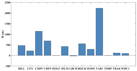
Figure 2.
IGS monitoring station elevation distribution.
2.2. Methods
2.2.1. K-Means Clustering-Assisted RBF Neural Network Region ZTD Modeling
RBF neural network is a three-layer feedforward network with a single hidden layer. The first layer corresponds to the input layer, which is composed of signal source nodes. The second layer is the hidden layer, and the number of nodes in this layer depends on the needs of the problem. The conversion function of neurons in the hidden layer, namely, the RBF, is a non-negative linear function with radial symmetry and attenuation to the center point. The third layer is the output layer, which is the response to the input mode. The basic idea is to use RBF as the “base” of the hidden unit to form the hidden layer space. The hidden layer transforms the input vector and transforms the low-dimensional input data into the high-dimensional space so that the linear indivisible problem in the low-dimensional space can be linearly separable in the high-dimensional space.
For ZTD region modeling, the problems to be solved are presented as follows. Giving a dataset and assuming that the dataset is generated by an unknown function , a function as close to as possible is learned by the dataset . For any feasible kernel functions , the function of the required solution can be expressed as:
where a is the parameter to be solved, and b is a constant.
From the sparse point of view, the RBF neural network adopts pruning ideas to achieve sparsity. First, an unsupervised learning process is performed on the input in the training data. A set of center vectors is selected in advance, and the number is less than the number of the original data. Subsequently, all the training data are used to learn the weights in Equation (1). The methods for selecting the RBF neural network center vector include orthogonal least-squares method [34], clustering method [35], and K-SVD method [36]. In the clustering method, not only the center vector can be determined, but also the sample covariances that belong to a certain type of data can be used as the covariance of RBF. In this paper, the K-means clustering method is used to obtain the center vector and covariance matrix [37]. The following anisotropic covariance matrix is defined as the kernel function:
where and represent the center vector and covariance matrix of the j-th RBF, which are obtained by K-means clustering, respectively:
- (1)
- Randomly select k objects, which indicate the initial centers of the k clusters to be divided. The number of k can be preferred by the k-fold cross-check or bootstrap method. In this paper, the value of k is selected as 1.
- (2)
- Calculate the distance between each point and the center point and find the center with the shortest distance as the new center point of each cluster.
- (3)
- Calculate the average value (centroid) of all objects in each cluster as the new center point of each cluster.
- (4)
- Calculate the distance between all objects and the new k centers again and redistribute all objects to each cluster according to the nearest distance principle.
- (5)
- Repeat the above steps until all cluster centers remain unchanged (the distance between the newly generated cluster and the previous cluster is less than a set threshold). This is the end of clustering.
After determining and , the function model to be established becomes:
where represents the weight vector.
It can be written in the form of the following observation equation:
where represents the true value of ZTD, e denotes other unmodeled noises, and the l × m matrix B is expressed as follows:
The m × 1 weight vector β in Equation (5) is estimated by using the least-squares method [14]:
The form of the observation equation can be seen as a trained estimator, that is, the regional ZTD model. In practical applications, the estimator is trained by using the ZTD data of the modeling station, and the corresponding ZTD can be estimated by inputting the coordinates and time of the prediction station inside or outside the area.
The ZTD region modeling flow chart is shown in Figure 3:
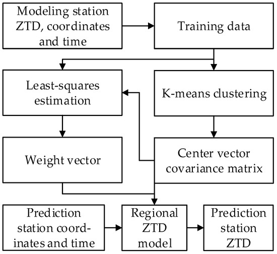
Figure 3.
ZTD region modeling flow chart.
2.2.2. Real-Time Parameters Updating LSTM Single-Station ZTD Modeling
LSTM neural network is a variant of recursive neural network (RNN), and LSTM expands its memory ability [38]. This feature enables LSTM to make ZTD prediction in an environment where meteorological information with evident advantages, stronger feasibility, and higher stability than the traditional ZTD acquisition method, such as Hopfield model, cannot be obtained [21].
However, the traditional LSTM cannot reasonably use the online ZTD value derived from GNSS techniques, such as PPP-RTK and RT-PPP. From the perspective of real-time ZTD modeling, a single-station ZTD modeling method with R-LSTM is given. The LSTM network refers to an online update mechanism for LSTM learning that minimizes the cost function. It can establish a practical model with only a small number of non-full life cycle samples (seconds to hours). The modeling idea is that: first, the reasonable use of known historical data is necessary to establish the LSTM prediction model. Second, when the actual online data are obtained, the corresponding prediction value can be achieved using the selected prediction. The new data at the next epoch can be used as the actual value of the prediction value. The error between the predicted value and the true value is added to the overall error of the sample. Finally, the error minimization method is used to update the model parameters iteratively. With the increasing use of online data, the model’s accuracy increases over time by updating the loop parameters. This modeling idea is more conducive to ZTD online modeling and prediction. The implementation steps of the R-LSTM prediction algorithm are presented as follows:
Assuming that the actual time series is , the improved LSTM calculation steps are presented as follows:
- (1)
- The actual time series is extended to , where n is the time series length, k is the sample dimension, n – k + 1 is the number of samples, and is the training data label. X is normalized:
- (2)
- Initialize network parameters and set super parameters:where and represent the initial weight and bias of the forgetting gate, respectively. The symbol rand ( ) represents a random function; and L and N represent the number of LSTM cell units and the number of neuron layers, respectively. Similarly, the initial weights and biases of the input gate, the output gate, the cell state, , , , , , , and other parameters also need to be initialized. Error_Cost and Max _ iter represent the error threshold and the maximum number of hyperparameter iterations, respectively.
- (3)
- Calculate what information needs to be forgotten from the cell state at time t – 1.where is the output of the forget gate. The symbol ( ) represents a sigmoid activation function. is the output value of the LSTM at the previous moment. is the input value of the network at the current moment. is the cell state at the previous moment. The symbol represents the point multiplication operation of the two vectors.
- (4)
- Calculate which input information can be left in the cell state at time t.where is the output of the input gate and determines what values will be updated. The symbol tanh ( ) represents a hyperbolic tangent activation function. is a vector of new candidate values created by the tanh function.
- (5)
- Calculate the cell state at time t.where is the result of the combined actions of the forget gate and the input gate on the cell states in Equations (9) and (10).
- (6)
- Calculate the network output at time t.where is the output of the output gate. is the predicted value at the current moment. Repeat Steps 3 to 6 to calculate the predicted values of all training samples.
- (7)
- Calculate the errors between the predicted values and the true values of all samples.where ( ) represents the cost function. The minimum value of the function in Equation (13), namely, the optimal solution error<Error_Cost, or the current number of iterations iter > Max_iter, are considered. Thus, the training ends. Otherwise, the BPTT algorithm is used to update the network parameters, and one is added to the number of iterations, and then the processing returns to Step 3 for circulation. It exits the loop until the error threshold or maximum number of iterations is reached. The following trained network parameters are saved:
- (8)
- Update parameters in real time according to online observation data. The new samples, and , perform the forward operation of the LSTM shown in Steps 3–6 to obtain the predicted value . When the data are collected, they can be used as the true value label of the predicted value to calculate the overall error:Then, the BPTT algorithm is used to update the model parameters to :where is the learning rate; and and are the gradient matrices and vectors of the weights and biases of each layer of neurons, respectively. The parameter initialization corresponds to the global optimal solution of the historical sample. Hence, when the new sample is added, the global optimal solution can be achieved again with only a few simple steps of updating.
The improved LSTM flow chart is shown in Figure 4:
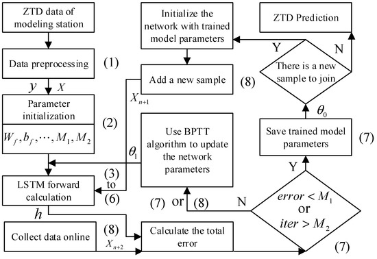
Figure 4.
ZTD single station modeling flow chart. Note: The serial number refers to the corresponding calculation steps.
In addition, the model can be applied to the early warning of severe convective weather. In Steps 6–8, when the predicted value of ZTD at the next sampling time reaches the warning value of severe convective weather, the warning information is issued to make emergency response in time. As a result, the economic losses to industrial and agricultural production will be reduced, and the utilization rate of water resources will be improved [39].
2.2.3. Regional/Single Station ZTD Combination Model
Based on the regional and single station ZTD model above, the regional/single station ZTD combination model is obtained by weighting:
where N is the total number of epochs. and represent the weights applied to the ZTD predicted by the regional and single station ZTD models in the i-th epoch, respectively. a and b represent the corresponding empirical weights, and a + b = 1. and represent the RMSE of the i − 1 predicted values of the regional and single station ZTD models before the i-th epoch, respectively.
The weights are gradually updated by comprehensively considering the new predicted value weights of the two models in the prediction process and the error level of the predicted values of the previous stage. According to the weighting scheme in Equation (18), the ZTD that corresponds to the combined model in the i-th epoch is presented as:
where represent the ZTD prediction values of the combined model, the regional model, and the single station model in the i-th epoch, respectively. is obtained by weighting the two other models.
2.2.4. Accuracy Evaluation Criteria
The RMSE, MAE, coefficient of determination (R2), and training time consumption (TTC) are used as the evaluation indexes of prediction model accuracy and efficiency. The computation is executed on a personal laptop with an Intel Core i7-10750H CPU at 2.60 GHz and with 16 GB of RAM. RMSE is used to measure the deviation between the predicted value and the true value of the model. MAE corresponds to the average of absolute error. No positive and negative offsets are observed because the deviation is absolute. Hence, the actual situation of the predicted value error can be reflected better. R2, also known as the goodness of fit in statistics, can measure the degree to which a variable is explained by another variable. Its value is between 0 and 1, which determines the degree of fitting among variables. The larger the value, the higher the correlation. TTC is used to measure the modeling efficiency of the model, which is particularly important for real-time modeling. The calculation formula of accuracy indicators, such as RMSE, MAE, and R2, are presented as follows:
where and are the true and predicted values on the test set, respectively. and are the corresponding average values; and N is the number of predicted samples.
3. Results
3.1. Regional Modeling Results
To verify the modeling accuracy and efficiency in the regional modeling, the modeling effects of different amounts of modeling data are compared and analyzed. Two sets of experiments were carried out. The first set of experiments (K-RBF-0) did not use historical data in the modeling process. The second set of experiments (K-RBF-5) used the five nearest consecutive epoch historical data in the modeling process. Figure 5 shows the accuracy and efficiency statistics results of 13 stations of K-RBF model for 90 days.
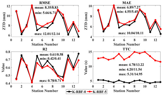
Figure 5.
K-RBF model accuracy and efficiency statistics results of K-RBF-0, K-RBF-5 experiments.
3.2. Single Station Modeling Results
The relationship between the amount of historical data and the accuracy and efficiency of modeling is analyzed using the conventional LSTM model as a reference to verify the modeling accuracy and modeling efficiency for the single station modeling. Taking the WHC1 station as an example, the ZTD data of the first 5, 12 × i (i = 1,2, …, 23) epochs of each day are selected for modeling, and the ZTD of the current epoch is used for accuracy verification. A total of 24 sets of experiments are recorded as Group1, Group2, …, Group24. Figure 6 shows the accuracy statistics results of R-LSTM and LSTM models for the 24 groups of experiments for 90 consecutive days. Figure 7 shows the true values, predicted values, and the differences of both changes in the two models in the Group1 experiment.
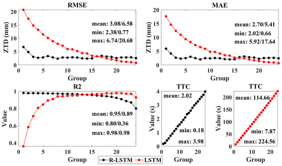
Figure 6.
Accuracy and efficiency statistics results of 24 groups of experiments of R−LSTM and LSTM models.
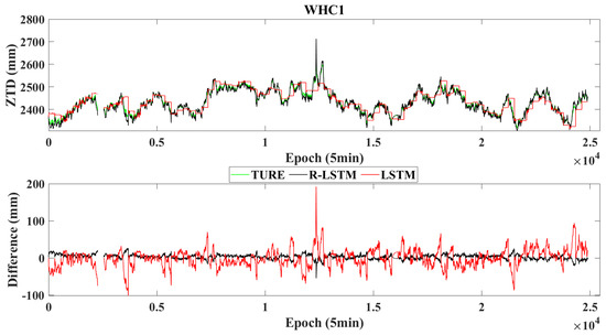
Figure 7.
Variations in the true values, predicted values, and errors of the R-LSTM and LSTM modeling in the Group1 experiment of WHC1 Station. Note: The data−free period in the figure is caused by the absence of true value data in this period.
3.3. Regional/Single Station Combination Modeling Results
To improve the real-time performance of modeling as much as possible, we select the K-RBF-0 group experimental method in the K-RBF regional modeling and the Group1 group experimental method in R-LSTM single station modeling for KR-RBF-STLM combined modeling. Table 1 and Figure 8 show the accuracy and efficiency statistics results of 13 stations for the three models for 90 days. The distribution of the modeling errors of various models is also compared and analyzed. Figure 9 shows the true values, predicted values, and the differences in the changes in the three models at the CIT1, JPLM, LBCH, and TORP stations. Figure 10 shows the error distribution of the three models at 13 stations for 90 days.

Table 1.
Statistical results of prediction accuracy and efficiency of K-RBF, R-LSTM, and KR-RBF-STLM models.
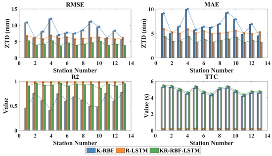
Figure 8.
Accuracy and efficiency changes in K-RBF, R-LSTM, and KR-RBF-STLM models at different stations.
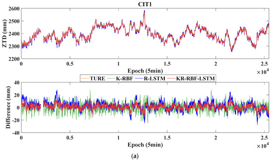
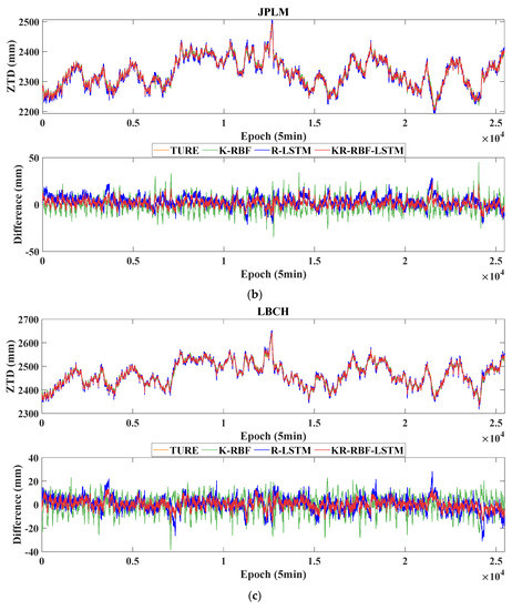
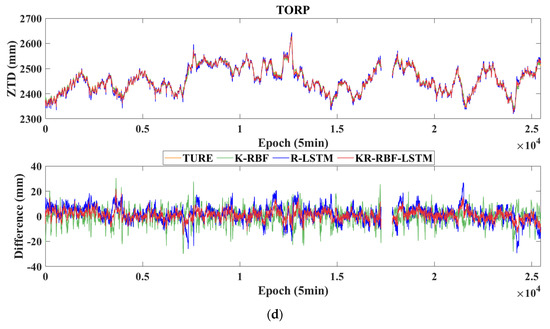
Figure 9.
Variations in the true values, predicted values, and errors of the K-RBF, R-LSTM, and KR-RBF-LSTM. (a) CIT1, Station number 2.; (b) JPLM, Station number 6.; (c) LBCH, Station number 7; (d) TORP, Station number 11. Note: The data−free period in the figure is caused by the absence of the true value data in this period.

Figure 10.
Error distribution of prediction results of K-RBF, R-LSTM, and KR-RBF-STLM models.
4. Discussion
4.1. Regional Modeling
(1) The mean, minimum (min), and maximum (max) of K-RBF-0 experiment are slightly higher than those of K-RBF-5. RMSE, MEA, and R2 are improved by 5.43%, 15.66%, 1.04%, 5.26%, 16.57%, 0.61%, 5.67%, 1.92%, and 8.22%. The mean, min, and max of TTC are greatly improved by 63.84%, 63.64%, and 64.49%, respectively. The main reason is that, with the increment in sample data, the total calculation time of the distance between each data and the center point in Equation (2) will increase. At the same time, the number of K-means clustering is not optimized and adjusted, thereby increasing time and slightly decreasing accuracy.
(2) The K-RBF-0 model has high accuracy and effectiveness. The means of RMSE, MAE, and R2 are 8.35 mm, 6.89 mm, and 0.61. Therefore, this model can meet the real-time forecasting needs for 4.78 s updates because the K-RBF model is simple, fast, robust, and highly accurate.
(3) For the K-RBF modeling, the accuracy of each station has certain differences. The distribution and density of the stations have a particular influence on the modeling accuracy. The accuracy of the station in the modeling area is higher than that outside the modeling area. For example, the accuracies of CIT1 (2), CMP9 (3), HOLP (5), and JPLM (6) stations are better than those of BILL (1), CRFP (4), SFDM (9), and TAB1 (10). The accuracy of the station in the dense area of the modeling station is higher than that in the sparse areas, such as TROP (11), TRAK (12) and BILL (1), and CRFP (4). Although they are all outside the modeling area, the modeling accuracy of the first two stations is better than those of the two latter stations because of the dense stations around the former. The main reason is that ZTD has a certain correlation in space. The more uniform the distribution of stations is, the higher the density is, and the higher the modeling accuracy is [40].
4.2. Single Station Modeling
(1) The RMSE and MAE of the R-LSTM model increase first and then stabilize with the increasing amounts of historical data. No significant increase was observed after the numbers of historical epochs exceeded 36. The mean values of the RMSE and MAE in Group3 to Group24 are 2.83 mm and 2.49 mm, respectively. R2 shows a slow downward trend, that is, from 0.98 to 0.80. TTC shows a gradual upward trend in mean, min, and max, which are equivalent to 2.02, 0.18, and 3.98 s, respectively.
(2) The RMSE, MAE, and TTC of the LSTM model show a gradual upward trend with increasing amounts of historical data, and R2 shows a gradual upward trend and a slow downward trend. When the number of historical epochs is 276, the RMSE and MAE are optimal at 0.77 mm and 0.66 mm, respectively. However, R2 is slightly lower than that of the previous group of experiment (Group23), and TTC is 56.44 times that of the R-LSTM model. When the number of historical epochs is 192, the accuracy of the two models is close, but the TTC difference is 56.81 times.
(3) When historical data are sufficient, the R-LSTM and LSTM prediction methods are effective. However, when the historical data are insufficient, the LSTM prediction effect is poor, and the R-LSTM method is still better. In the Group1 experiment (the experimental results are shown in Figure 8), the RMSE, MAE, R2, and TTC of the R-LSTM model are 6.74 mm, 5.92 mm, 0.98, and 0.18 s, respectively. Compared with those of the LSTM model, these values are improved by 67.43%, 66.42%, 63.33%, and 97.70%, respectively. The R-LSTM model can predict the trend of ZTD, whereas the prediction results of the LSTM model gradually changed linearly. For the epoch of dramatic changes in ZTD, such as the 3679th, 12,354th, and 21,489th epochs, the prediction results of R-LSTM are significantly better. The main reason is that the training samples of the LSTM model are insufficient in this case, and the parameters of the R-LSTM model can be updated in real time.
4.3. Regional/Single Station Combination Modeling
(1) The mean, min, and max of the RMS, MAE, R2, and KR-RBF-LSTM relative to K-RBF are improved by 47.70%, 33.94%, 56.22%, 47.72%, 31.20%, 56.16%, 33.51%, 51.54%, and 19.10%; TTC is increased by 3.71%, 4.28%, and 3.30%. Compared with R-LSTM, the mean, min, and max of RMS and MAE are improved by 28.48%, 34.47%, and 22.93%, as well as 31.29%, 36.43%, and 25.68%, respectively. R2 is reduced by 5.43%, 11.73%, and 2.24%, and TTC is increased by 96.29%, 95.94%, and 96.20%. In general, the accuracy of the KR-RBF-LSTM model is the best mainly because the combination model relates the advantages of the two models. That is, K-RBF can consider the spatial correlation of the stations, and R-LSTM can consider the temporal correlation of the stations. When the two are combined, the spatial and temporal correlations can be considered. Specifically, this advantage is more obvious in the epoch where the ZTD changes greatly. The R-LSTM model has the best real-time performance. The main reason is that the parameters of the model can be updated in real time and can quickly reach the global optimal state. Its training samples are only five historical data of a certain station, whereas the training data of other models are 2.40 or 3.40 times greater than that. Compared with the BP neural network model, the K-RBF model can avoid the problem of the unstable model and time-consuming training due to the lack of training samples. It exhibits a certain improvement in terms of accuracy and efficiency [24,41,42].
(2) The distribution of modeling stations will affect the K-RBF modeling effect to a certain extent, and the influence on the KR-RBF-LSTM model weakens. No significant difference is observed in the accuracy indicators of each R-LSTM station. The main reason is that the ZTD has spatial and temporal correlations. The strength of spatial correlation varies for the distribution of different stations. The regional model considers the spatial correlation of stations, and the combined model further considers the time correlation of stations. However, the influence of other stations is ignored in the single station model, which is only related to the small amount of historical data of the station and the physical change degree of the ZTD itself.
(3) The errors of the three models are subject to normal distribution, indicating that the models established in this paper are reasonable. At the same time, the error distribution of the KR-RBF-LSTM model is better than those of K-RBF and R-LSTM, and its standard deviation (STD) is improved by 50.98% and 28.43%, respectively.
(4) Although ZTD and station elevation are correlated [20] and the elevation of some stations in the study area fluctuates greatly, the prediction accuracy of the three models does not show a strong correlation with the station elevation. The main reason is that the K-RBF and KR-RBF-LSTM models consider the influence of elevation. The R-LSTM model can gradually optimize and update the established model parameters according to the ZTD data obtained at each epoch.
(5) The real-time/near real-time application of the three models can be selected according to the user’s needs. Under the condition that no historical data are in the prediction station, the real-time ZTD data of the regional monitoring station exist around it, and the K-RBF model can be selected to provide high-precision ZTD enhancement products for RTK, PPP-RTK, and other positioning modes. Under the condition that the prediction station has a small amount of historical data (which can be obtained by empirical model), but no ZTD data of regional monitoring stations are around it, the R-LSTM model can be selected to improve the prediction accuracy of real-time PPP-based ZTD and serve the extreme weather forecast. KR-RBF-LSTM model can be used to meet the needs of RTK, real-time PPP, PPP-RTK, and other high-precision real-time positioning modes under the condition that the prediction station has a small amount of historical data and real-time ZTD data of regional monitoring station around it. Specifically, in a short time (such as within 2 min), the demand for mm-level positioning accuracy in the elevation direction, such as mining subsidence monitoring, is urgent.
5. Conclusions
A regional/single station ZTD combination prediction model is proposed, aiming at the problem that the traditional BP neural network modeling is inefficient and has local optimum and that the traditional LSTM modeling cannot effectively use the data of a non-full life cycle to establish an excellent ZTD prediction model and cannot reasonably use the online data. The model considers the ZTD spatiotemporal information and applies algorithms of the RBF neural network based on K-means clustering and LSTM with real-time parameter updating. The model mainly solves the problem of online modeling and model correction of small sample data in regional real-time/near real-time ZTD modeling. Taking the ZTD data of 13 IGS stations in Southern California for 90 consecutive days as an example (5 min sampling interval), the prediction performance of the proposed combined model in regional real-time ZTD modeling is verified. Compared with K-RBF, the RMSE, MAE, and STD of KR-RBF-LSTM are improved by 47.70%, 47.20%, and 50.98%, respectively. Compared with R-LSTM, the RMSE, MAE, and STD are improved by 24.48%, 31.29%, and 28.43%, respectively. Compared with the traditional BP model, the accuracy and efficiency of K-RBF exhibited a certain improvement. Compared with LSTM, the RMSE and MAE of R-LSTM are improved by 66.43% and 66.42%, respectively.
The research results of this paper have high reference values for PPP-RTK, RT-PPP, RTK, and extreme weather forecasting based on regional atmospheric enhancement products. Based on the current work, we can perform further research in the future. First, the ZTD prediction value of the model with better historical RMSE performance is weighted higher, and the ZTD prediction value of the combined model may not necessarily take the optimal value. If the weight in the combined model is adaptively adjusted by using the relevant optimization algorithm, then the prediction accuracy and stability of the model can be improved further. Second, the accuracy and efficiency of the regional and single station models are further improved by optimizing the K-means algorithm and by seeking more effective R-LSTM parameter optimization methods. Third, due to the lack of clear physical mechanism of artificial intelligence algorithms, such as that in this paper, the research on the dynamic change and formation mechanism of atmospheric water vapor is strengthened. From the perspective of meteorology, hydrology, geography, and other disciplines, the prediction model is established on the basis of strict physical causes. It is the focus of extreme weather forecast and climate change research to serve the response and feedback of carbon, nitrogen, and water cycle to climate change and other multidisciplinary scientific research.
Author Contributions
Conceptualization, X.Y. (Xu Yang) and Y.L.; methodology, X.Y. (Xu Yang) and X.Y. (Xuexiang Yu); software, X.Y. (Xu Yang) and X.Y. (Xuexiang Yu); validation, X.Y. (Xu Yang), Y.L. and X.Y. (Xuexiang Yu); formal analysis, X.Y. (Xu Yang) and Y.L.; investigation, X.Y. (Xu Yang) and H.T.; resources, X.Y. (Xu Yang) and J.Y.; data curation, X.Y. (Xu Yang) and M.Z.; writing—original draft preparation, X.Y. (Xu Yang); writing—review and editing, X.Y. (Xu Yang), Y.L., X.Y. (Xuexiang Yu), H.T., J.Y. and M.Z.; visualization, X.Y. (Xu Yang) and M.Z.; supervision, Y.L. and M.Z.; project administration, X.Y. (Xu Yang); funding acquisition, X.Y. (Xu Yang), Y.L., X.Y. (Xuexiang Yu) and J.Y. All authors have read and agreed to the published version of the manuscript.
Funding
This work was supported by the “Key Laboratory of Aviation-aerospace-ground Cooperative Monitoring and Early Warning of Coal Mining-induced Disasters of Anhui Higher Education Institutes (Anhui University of Science and Technology) (No.KLAHEI202204)”, “Anhui Province Natural Science Foundation (No.2208085QD115, 2008085MD114)”, “Major Special Projects of Science and Technology in Anhui Province (No.202103a05020026)”, “Key Research and Development Projects of Anhui Province (No.202104a07020014)”, “Open Foundation of the Key Laboratory of Universities in Anhui Province for Prevention of Mine Geological Disasters (No.2022-MGDP-08)”, “Key Natural Science Projects of Anhui Provincial Department of Education (No.KJ2020A0311, 2022AH050820)”, “Coal Industry Engineering Research Center of Mining Area Environmental And Disaster Cooperative Monitoring, Anhui University of Science and Technology (Anhui University of Science and Technology) (No.KSXTJC202005, KSXTJC202207)”, and “Introduction of Talent Research Startup Fund Project of Anhui University of Science and Technology (No.2019, 13200458)”.
Institutional Review Board Statement
Not applicable.
Informed Consent Statement
Not applicable.
Data Availability Statement
The data used to support the findings of this study are available from the corresponding author upon request.
Acknowledgments
The authors appreciate the International GNSS Service for providing relevant data and products.
Conflicts of Interest
The authors declare no conflict of interest.
Abbreviations
| GNSS | Global navigation satellite system |
| GPS | Global positioning system |
| ZTD | Zenith tropospheric delay |
| ZHD | Zenith hydrostatic delay |
| ZWD | Zenith wet delay |
| BP | Back propagation |
| LSTM | Long short-term memory |
| LSTM E/D | Long short-term memory encoder decoder |
| RBF | Radial basis function |
| K-RBF | RBF neural network assisted by the K-means cluster algorithm |
| R-LSTM | LSTM of real-time parameter updating |
| KR-RBF-LSTM | K-RBF and R-LSTM |
| RMSE | Root-mean-square error |
| STD | Standard deviation |
| MAE | Mean absolute error |
| MAPE | Mean absolute percentage error |
| R2 | Coefficient of determination |
| TTC | Training time consumption |
| PWV | Precipitable water vapor |
| NWP | Numerical weather prediction |
| ML | Machine learning |
| ANFIS | Adaptive network-based fuzzy inference system |
| ANN | Artificial neural network |
| LSSVM | Least-squares support vector machine |
| PCA | Principal component analysis |
| ICA | Independent component analysis |
| GGOS | Global geodetic observing system |
| CNN | Convolutional neural network |
| KNN | K-nearest neighbor |
| GP | Gaussian processes |
| ERA5 | Fifth-generation European Center for Medium-range Weather Forecast reanalysis |
| PPP | Precision point positioning |
| RT-PPP | Real-time precision point positioning |
| RTK | Real-time kinematic positioning |
| CORS | Continuously-operating reference station |
| PPP-RTK | Integer ambiguity resolution-enabled precise point positioning |
| IGS | International GNSS Service |
| DOY | Day of the year |
References
- Van Baelen, J.; Aubagnac, J.P.; Dabas, A. Comparison of near-real time estimates of integrated water vapor derived with GPS, radiosondes, and microwave radiometer. J. Atmos. Ocean. Technol. 2005, 22, 201–210. [Google Scholar] [CrossRef]
- Brenot, H.; Neméghaire, J.; Delobbe, L.; Clerbaux, N.; Meutter, P.D.; Deckmyn, A.; Delcloo, A.; Frappez, L.; Roozendael, M.V. Preliminary signs of the initiation of deep convection by GNSS. Atmos. Chem. Phys. 2013, 13, 5425–5449. [Google Scholar] [CrossRef]
- Tunali, E. Water vapor monitoring with IGS RTS and GPT3/VMF3 functions over Turkey. Adv. Space Res. 2022, 69, 2376–2390. [Google Scholar] [CrossRef]
- Troller, M.; Geiger, A.; Brockmann, E.; Bettems, J.M.; Bürkia, B.; Kahle, H.-G. Tomographic determination of the spatial distribution of water vapor using GPS observations. Adv. Space Res. 2006, 37, 2211–2217. [Google Scholar] [CrossRef]
- Zangvil, A.; Portis, D.H.; Lamb, P.J. Investigation of the large-scale atmospheric moisture field over the midwestern United States in relation to summer precipitation. Part II: Recycling of local evapotranspiration and association with soil moisture and crop yields. J. Clim. 2004, 17, 3283–3301. [Google Scholar] [CrossRef]
- Park, H.J.; Shin, D.B.; Yoo, J.M. Atmospheric water balance over oceanic regions as estimated from satellite, merged, and reanalysis data. J. Geophys. Res.-Atmos. 2013, 118, 3495–3505. [Google Scholar] [CrossRef]
- National Research Council. New Research Opportunities in the Earth Sciences; National Academy Press: Washington, DC, USA, 2012; Available online: http://www.nap.edu/openbook.php?record_id=13236 (accessed on 31 October 2014).
- Suni, T.; Guenther, A.; Hansson, H.C.; Kulmala, M.; Andreae, M.O.; Arneth, A.; Artaxo, P.; Blyth, E.; Brus, M.; Ganzeveld, L.; et al. The significance of land-atmosphere interactions in the Earth system—iLEAPS achievements and perspectives. Anthropocene 2015, 12, 69–84. [Google Scholar] [CrossRef]
- Bevis, M.; Businger, S.; Herring, T.A.; Rocken, C.; Anthes, R.A.; Ware, R.H. GPS meteorology: Remote sensing of atmospheric water vapor using the Global Positioning System. J. Geophys. Res.-Atmos. 1992, 97, 15787–15801. [Google Scholar] [CrossRef]
- Guerova, G.; Jones, J.; Douša, J.; Dick, G.; Haan, S.D.; Pottiaux, E.; Bock, O.; Pacione, R.; Elgered, G.; Vedel, H.; et al. Review of the state of the art and future prospects of the ground-based GNSS meteorology in Europe. Atmos. Meas. Tech. 2016, 9, 5385–5406. [Google Scholar] [CrossRef]
- Zhang, K.; Manning, T.; Wu, S.; Rohm, W.; Silcock, D.; Choy, S. Capturing the Signature of Severe Weather Events in Australia Using GPS Measurements. IEEE J. Sel. Top. Appl. Earth Obs. Remote Sens. 2015, 8, 1839–1847. [Google Scholar] [CrossRef]
- Liu, J.; Chang, Z.; Zheng, H. Analysis on the performances of the GNSS tropospheric delay correction models. E3S Web Conf. 2022, 360, 01043. [Google Scholar] [CrossRef]
- Li, W.; Yuan, Y.; Ou, J.; He, Y. IGGtrop_SH and IGGtrop_rH: Two Improved Empirical Tropospheric Delay Models Based on Vertical Reduction Functions. IEEE Trans. Geosci. Remote Sens. 2018, 56, 5276–5288. [Google Scholar] [CrossRef]
- Ghaderpour, E.; Pagiatakis, S.D.; Hassan, Q.K. A Survey on Change Detection and Time Series Analysis with Applications. Appl. Sci. 2021, 11, 6141. [Google Scholar] [CrossRef]
- Ma, Y.; Liu, T.; Xu, G.; Lu, Z. Apparent Short-Period GNSS-ZTD Disturbance Correlated with Precipitation Events. IEEE Geosci. Remote Sens. 2022, 19, 1006305. [Google Scholar] [CrossRef]
- Ghaderpour, E. Least-squares Wavelet and Cross-wavelet Analyses of VLBI Baseline Length and Temperature Time Series: Fortaleza–Hartebeesthoek–Westford–Wettzell. Publ. Astron. Soc. Pac. 2021, 133, 014502. [Google Scholar] [CrossRef]
- Shamshiri, R.; Motagh, M.; Nahavandchi, H.; Haghighi, M.H.; Hoseini, M. Improving tropospheric corrections on large-scale Sentinel-1 interferograms using a machine learning approach for integration with GNSS-derived zenith total delay (ZTD). Remote Sens. Environ 2020, 239, 111608. [Google Scholar] [CrossRef]
- Wilgan, K.; Geiger, A. High-resolution models of tropospheric delays and refractivity based on GNSS and numerical weather prediction data for alpine regions in Switzerland. J. Geodesy 2019, 93, 819–835. [Google Scholar] [CrossRef]
- Chen, J.; Wang, J.; Wang, J.; Tan, W.; Observation, S.A. SHAtrop: Empirical ZTD Model Based on CMONOC GNSS Network. Geomat. Inf. Sci. Wuhan Univ. 2019, 44, 1588–1595. [Google Scholar]
- Zhao, Q.; Su, J.; Xu, C.; Yao, Y.; Zhang, X.; Wu, J. High-precision ZTD model of altitude-related correction. IEEE J. Sel. Top. Appl. Earth Obs. Remote Sens. 2023, 16, 609–621. [Google Scholar] [CrossRef]
- Chkeir, S.; Anesiadou, A.; Mascitelli, A.; Biondi, R. Nowcasting extreme rain and extreme wind speed with machine learning techniques applied to different input datasets. Atmos. Res. 2023, 282, 106548. [Google Scholar] [CrossRef]
- Zhang, H.; Yao, Y.; Hu, M.; Xu, C.; Su, X.; Che, D.; Peng, W. A Tropospheric Zenith Delay Forecasting Model Based on a Long Short-Term Memory Neural Network and Its Impact on Precise Point Positioning. Remote Sens. 2022, 14, 5921. [Google Scholar] [CrossRef]
- Xiao, X.; Lv, W.; Han, Y.; Lu, F.; Liu, J. Prediction of CORS Water Vapor Values Based on the CEEMDAN and ARIMA-LSTM Combination Model. Atmosphere 2022, 13, 1453. [Google Scholar] [CrossRef]
- Xu, T.; Li, S.; Wang, S.; Jiang, N. Improved tropospheric delay model for China using RBF neural network and meteorological data. Acta Geod. Cartogr. Sin. 2022, 51, 1690–1707. [Google Scholar]
- Wang, Y.; Zhang, L.; Yang, J. Study on prediction of zenith tropospheric delay by use of BP neural network. J. Geod. Geodyn. 2011, 31, 134–137. [Google Scholar]
- Xiao, G.; Ou, J.; Liu, G.; Zhang, H. Construction of a regional precise tropospheric delay model based on improved BP neural network. Chin. J. Geophys. 2018, 61, 3139–3148. (In Chinese) [Google Scholar]
- Li, S. GNSS Tropospheric Delay Modeling and Prediction Based on Machine Learning; Chang’an University: Xi’an, China, 2021. [Google Scholar]
- Shi, Y.; Wu, F.; Zhu, H.; Han, X. Prediction of tropospheric delay based on the LSTM model of Keras platform. GNSS World China 2020, 45, 115–122. [Google Scholar]
- Zhang, Q.; Li, F.; Zhang, S.; Li, W. Modeling and Forecasting the GPS Zenith Troposphere Delay in West Antarctica Based on Different Blind Source Separation Methods and Deep Learning. Sensors 2020, 20, 2343. [Google Scholar] [CrossRef] [PubMed]
- Li, S.; Xu, T.; Xu, Y.; Jiang, N.; Bastos, L. Forecasting GNSS Zenith Troposphere Delay by Improving GPT3 Model with Machine Learning in Antarctica. Atmosphere 2022, 13, 78. [Google Scholar] [CrossRef]
- Zhang, H.; Yao, Y.; Xu, C.; Xu, W.; Shi, J. Transformer-Based Global Zenith Tropospheric Delay Forecasting Model. Remote Sens. 2022, 14, 3335. [Google Scholar] [CrossRef]
- Zheng, Y.; Lu, C.; Wu, Z.; Liao, J.; Zhang, Y.; Wang, Q. Machine learning-based model for real-time GNSS precipitable water vapor sensing. Geophys. Res. Lett. 2022, 49, e2021GL096408. [Google Scholar] [CrossRef]
- Chen, B.; Liu, Z.; Wong, K.; Woo, W.C. Detecting Water Vapor Variability during Heavy Precipitation Events in Hong Kong Using the GPS Tomographic Technique. J. Atmos. Ocean. Technol. 2017, 34, 1001–1019. [Google Scholar] [CrossRef]
- Chen, S.; Cowan, C.F.N.; Grant, P.M. Orthogonal least squares learning algorithm for radial basis function networks. IEEE Trans. Neural Netw. 1991, 2, 302–309. [Google Scholar] [CrossRef] [PubMed]
- Moody, J.; Darken, C. Fast Learning in Networks of Locally-Tuned Processing Units. Neural Comput. 1989, 1, 281–294. [Google Scholar] [CrossRef]
- Aharon, M.; Elad, M.; Bruckstein, A. K-SVD: An Algorithm for Designing Overcomplete Dictionaries for Sparse Representation. IEEE Trans. Signal Process. 2006, 54, 4310–4323. [Google Scholar] [CrossRef]
- Jain, A.K. Data clustering: 50 years beyond K-means. Pattern Recognit. Lett. 2010, 31, 651–666. [Google Scholar] [CrossRef]
- Yu, Y.; Si, X.; Hu, C.; Zhang, J. A Review of Recurrent Neural Networks: LSTM Cells and Network Architectures. Neural Comput. 2019, 31, 1235–1270. [Google Scholar] [CrossRef]
- Li, L.; Kuang, C.; Zhu, J.; Chen, W.; Chen, Y.; Long, S.; Li, H. Rainstorm nowcasting based on GPS real-time precise point positioning technology. Chin. J. Geophys. 2012, 55, 1129–1136. [Google Scholar]
- Wang, S.; Li, B.; Gao, Y.; Gao, Y.; Guo, H. A comprehensive assessment of interpolation methods for regional augmented PPP using reference networks with different scales and terrains. Measurement 2020, 150, 107067. [Google Scholar] [CrossRef]
- Li, S.; Xu, T.; Jiang, N. Tropospheric Delay Modeling Based on Multi-source Data Fusion and Machine Learning Algorithms. In Proceedings of the China Satellite Navigation Conference (CSNC 2021), Nanchang, China, 26–28 May 2021; Lecture Notes in Electrical Engineering. Springer: Berlin/Heidelberg, Germany, 2021; Volume 772, pp. 145–158. [Google Scholar]
- Qiao, X.; Chang, W.; Zhou, S.; Lu, X. A prediction model of hard landing based on RBF neural network with K-means clustering algorithm. In Proceedings of the 2016 IEEE International Conference on Industrial Engineering and Engineering Management (IEEM), Bali, Indonesia, 4−7 December 2016; pp. 462–465. [Google Scholar]
Disclaimer/Publisher’s Note: The statements, opinions and data contained in all publications are solely those of the individual author(s) and contributor(s) and not of MDPI and/or the editor(s). MDPI and/or the editor(s) disclaim responsibility for any injury to people or property resulting from any ideas, methods, instructions or products referred to in the content. |
© 2023 by the authors. Licensee MDPI, Basel, Switzerland. This article is an open access article distributed under the terms and conditions of the Creative Commons Attribution (CC BY) license (https://creativecommons.org/licenses/by/4.0/).