Article

An Improved Ensemble-Strategy-Assisted Wind Speed Prediction Method for Railway Strong Wind Warnings

1
Chongqing Wukang Technology Co., Ltd., Chongqing 404100, China
2
School of Civil Engineering, Chongqing Jiaotong University, Chongqing 400074, China
3
College of Engineering and Technology, Southwest University, Chongqing 400715, China
*
Authors to whom correspondence should be addressed.
Atmosphere 2023, 14(12), 1787; https://doi.org/10.3390/atmos14121787
Submission received: 13 November 2023 / Revised: 23 November 2023 / Accepted: 1 December 2023 / Published: 5 December 2023

Abstract

:
Reliable short-term wind speed prediction is one of the core technologies in the strong wind warning system for railway applications, which is of great significance for ensuring the safety of high-speed train operations and ancillary railway facilities. To improve forecasting accuracy, decomposition-based methods have attracted extensive attention due to their superior ability to address complex data characteristics (e.g., nonstationarity and nonlinearity). Currently, there are two pre-processing schemes for decomposition-based methods, i.e., one-time decomposition and real-time decomposition. In order to apply them better, this paper first expounds the difference between them, based on a combination of DWT (discrete wavelet transform) and CKDE (conditional kernel density estimation). The results show that although the one-time decomposition-based method has an unexceptionable accuracy, it only can provide offline prediction and thus may not be practical. The real-time decomposition-based method possesses stronger practicability and is able to provide online prediction, but it has limited accuracy. Then, an improved ensemble strategy is developed by optimizing the selection of appropriate decomposed components to conduct the prediction on the basis of real-time decomposition. This improved ensemble strategy provides an effective guidance for this selective combination, including taking historical information into consideration in the data. Finally, numerical examples and practicality analysis using two groups of measured wind speed data demonstrate that the proposed method is effective in providing high-precision online wind speed prediction. For example, compared with CKDE, the average degrees of improvement achieved by the proposed method in terms of MAE, RMSE, and MRPE, are 16.25%, 17.66%, and 16.93, respectively, while those compared with the traditional real-time decomposition method are 17.11%, 18.54%, and 16.84, respectively.

1. Introduction

In recent years, a large number of high-speed rail projects have been constructed around the world, and the corresponding scale of development is very rapid [1,2]. According to a statistical report by China Railway, China’s railway service length had reached 155,000 km, including 42,000 km of high-speed railways, by the end of 2022. However, due to the light weight of high-speed train carriages and their high operating speeds, operational high-speed trains inevitably encounter large lift forces under the action of strong winds. Therefore, they are highly susceptible to derailment and overturning [3,4,5], which can lead to significant casualties and huge economic losses [6,7]. Meanwhile, safety and reliability of structures (e.g., bridges and transmission Lines) under the action of strong winds have also become an increasingly serious topic [8,9,10,11,12,13,14,15]. One of effective methods to addressing this predicament is the accurate prediction of strong winds (i.e., short-term wind speed prediction), which will enable the railway dispatching system to adjust dispatch plans in a timely manner [16]. Therefore, short-term wind speed prediction is one of the most important techniques in high-speed railway warning systems, which also plays a significant role in ensuring the operational safety of high-speed trains [17,18,19].
To perform short-term wind speed prediction, many attempts have been made to generate a plethora of forecasting methods [20,21]. Generally, these methods can be categorized into four different kinds, including physical models, statistical models, artificial intelligence- or machine learning-based models, and hybrid models [22]. Physical models mainly utilize meteorological data (such as temperature, humidity, air pressure, etc.) to carry out wind speed prediction. One representative model is the numerical weather prediction model (numerical weather prediction, NWP) [23]. However, this type of model requires a large amount of meteorological data and computational resources and is merely suitable for long-term wind speed prediction [24]. Statistical models (i.e., time series models) can directly analyze the linear relationship between historical wind speed records, from which the corresponding forecasting models are established. These models generally possess a simple and effective structure, and have been widely used in short-term wind speed prediction. They include the auto-regressive (AR) model, moving average (MA) model, auto-regressive moving average (ARMA) model, and difference auto-regressive integrated moving average (ARIMA) model [25,26]. However, these models usually perform well under the assumption of stationary time series and cannot address the prediction of wind speed data with high nonlinear features [27]. Fortunately, artificial intelligence- or machine learning-based models, such as Kalman filters [28], artificial neural networks (ANN) [29], fuzzy logic [30], support vector machines (SVM) [31], deep learning (DL) [32], etc., can effectively explain the nonlinear features embedded in the data. These models have been successfully applied in the field of wind speed prediction. However, the before-mentioned models mostly belong to the parametric model category and generally include complex parameter optimization processes [33,34]. Meanwhile, they easily fall into the problems of local optimization, overfitting, and low rate of convergence [35]. Recently, conditional kernel density estimation (CKDE) has been able to determine the probability density function (PDF) of the target variable and use it as a basis for addressing the time series prediction problem [36]. This method has data-driven attributes and can directly use the sample data to estimate the PDF without any parametric assumption. In addition to the simple single-modal density distribution problem, it can effectively deal with problems of multi-modal or skewed density distributions [22]. Therefore, the CKDE model can not only avoid errors and computational resources caused by parameter optimization processes, but also respond well to the non-linear and non-Gaussian characteristics hidden in wind speed time series [37]. Considering the advantages of CKDE, the integration of this method into wind speed prediction may be promising and challenging.
According to [38,39,40,41,42,43], wind speed time series usually present multiple characteristics (e.g., linearity, nonstationarity, nonlinearity, etc.). In this scenario, the above-mentioned single models may not provide satisfactory forecasting results. To pursue higher forecasting accuracy, the combination of different component methods (i.e., hybrid models) has attracted more and more attention. These hybrid methods can take advantage of the strength of each component model. There are four different hybrid models including decomposition-based models, parameter optimization-based models, weight allocation-based models, and error correction-based models [44]. Due to strong volatility and stationarity of wind speed time series, hybrid models based on signal pretreatment techniques are extensively employed. These pretreatment techniques main are empirical mode decomposition (EMD) [16], fast ensemble EMD (FEEMD) [45], discrete wavelet transform (DWT) [46], wavelet packet decomposition (WPD) [47], empirical wavelet transform (EWT) [48], variational mode decomposition (VMD) [49], and their developed versions. Generally, these types of hybrid models first apply signal pretreatment techniques to decompose the raw wind speed data into different stationary and regular subsequences. Then, one or several appropriate models are established for training each subsequence and performing the corresponding prediction. Finally, the summation of all individual predictions in a linear manner can be regarded as the target prediction result [50]. For example, Liu et al. [51] used four different decomposition techniques (i.e., EMD, FEEMD, DWT, and WPD) and extreme learning machine (ELM) to implement the prediction of short-term wind speeds, and the forecasting result indicated that the accuracy of these decomposition-based models was superior to that of single models. In most relevant studies, the decomposition is only conducted once for the original data, and each decomposed subsequence is divided into training and testing sets (i.e., one-time decomposition). Although one-time decomposition-based models feature extremely high accuracy, the decomposition takes the future information into consideration and can only provide offline prediction [52]. Therefore, this method may not be practical. In contrast, the real-time decomposition-based method has a stronger practicability and is able to provide online prediction, but it forecasting accuracy is generally limited and sometimes even inferior to that of single models [50]. The possible reasons for this limited accuracy may be ascribed to the effect of the endpoint effect, mode mixing, improper or varying decomposition level number, and illusory components [24]. Meanwhile, the ensemble pattern (i.e., the direct summation of all individual predictions) may not be effective, while the selective ensemble of several individual predictions generally presents satisfactory results [53]. However, the difference between one-time decomposition-based methods and real-time decomposition-based methods is rarely reported, and the selective ensemble pattern in these methods sometimes depends on the user’s experience, which generally lacks a theoretical basis.
From the above literature review, several main problems in the current methods of short-term wind speed prediction are summarized below: ① Physical models require a large quantity of meteorological data and computational resources, and are merely suitable for long-term wind speed prediction; ② statistical models only can perform well for the prediction of wind speed time series with strong linear and stationary characteristics; ③ artificial intelligence or machine learning models can capture linear and complex nonlinear characteristics in the wind speed data, but they cannot effectively address nonstationary characteristics in the data and their performance is vulnerable to model parameters; ④ although two kinds of decomposition-based methods have been widely used, the differences between then are rarely clarified, which sometimes brings about unsuitable applications. Meanwhile, forecasting accuracy is strongly related to the ensemble pattern of subsequence predictions, which generally lack a theoretical basis.
This paper first introduces the nonparametric CKDE model as the predictor and reviews the details of two traditional decomposition-based models and the differences between them on the basis of DWT. Then, the performance evaluation of these two methods is conducted based on measured wind speed data. Further, an improved ensemble-strategy-assisted real-time decomposition method is developed for short-term wind speed prediction, which can optimally select the decomposed components for ensemble predictions. Finally, numerical examples are performed to illustrate the performance of the proposed method. The forecasting results show that this improved method has higher prediction accuracy in comparison with traditional real-time decomposition-based models and the single CKDE model. For example, compared with CKDE, the average degrees of improvement realized by the proposed method in terms of MAE, RMSE, and MRPE are 16.25%, 17.66%, and 16.93, respectively, while those compared with the traditional real-time decomposition method are 17.11%, 18.54%, and 16.84, respectively.

2. Methodology

2.1. Discrete Wavelet Transform

As a convenient and efficient technique of multiscale signal processing, discrete wavelet transform (DWT) has been widely used in the analysis of nonlinear and nonstationary signals [54]. This technique can decompose the signal into specified quantity subsequences with different frequency bandwidths by employing a group of basis functions. These basis functions generally result from a series of translation and expansion operations based on the pre-specified mother wavelet function [54]. For the original wind speed time series v 1 , v 2 , , v n (denoted as v[n]), DWT can decompose this signal into a number of approximation and detail components, i.e., [55]
v n = D 1 + D 2 + . . . + D k + A k
where n represents the number of original data points; k + 1 represents the specified decomposition level of DWT; D1, D2,..., Dk represent the detail components; and Ak stands for the approximation component.
With the augmentation of decomposition level numbers, the frequency on the corresponding subsequence gradually decreases, and thus the frequency overlap between two adjacent subsequences can be addressed to some extent [54]. Meanwhile, the number of decomposition levels can be set in advance. Therefore, this technique has the ability to address the time-frequency analysis of both single-channel data and multi-channel data [56]. In this technique, the critical problem is determining the mother wavelet function. According to [54], the Daubechies 10 wavelet has exhibited superiority in analyzing the wind speed time series, which is still used for the decomposition and reconstruction in this paper. The detailed illustration of DWT can be found in [55].

2.2. Conditional Kernel Density Estimation

After the decomposition by DWT is completed, the CKDE model is established for every decomposed subsequence. In this model, any assumption regarding the relationship between input and output variables can be avoided [57]. In addition to having the ability to describe the linear characteristics in the data, this model embodies an obvious advantage in addressing the data with multimodal or skewed probability distributions, and thus can explain the nonlinear or non-Gaussian characteristics in the wind speed time series [44]. The following gives the detailed modeling process of CKDE in wind speed prediction.
For any decomposed subsequence x ( t ) , t = 1 , 2 , 3 , , n , a series of input–output pairs with the L-step ahead forecasting task can be constructed, i.e.,
x 1 x i x N = x ( 1 ) x ( m ) x ( i ) x ( i + m 1 ) x ( N ) x ( n L ) ;   y 1 y i y N = x ( m + L ) x ( i + L + m 1 ) x ( n )
where x i , i = 1 , 2 , , N ;   N = n m L + 1 denotes the m-dimensional input variable and y i stands for the one-dimensional output variable. On this basis, the joint probability density distribution of ( x , y ) can be expressed as:
f ^ ( x , y ) = 1 N H X H Y i = 1 N K m H X 1 ( x x i ) K H Y 1 ( y y t )
where K m is the m-dimensional kernel function and the Gaussian function is commonly used because of its simple structure and easy application; H X and H Y are the diagonal bandwidth matrixes for input and output variables, respectively [36]. These bandwidth matrixes are critical for ensuring modeling quality, and generally can be obtained via the normal reference criterion (NRC), i.e., [44]
H X = d i a g H q ; H Y = σ Y 4 / m + 2 N 1 / m + 4 ; H q = σ q 4 / m + 2 N 1 / m + 4 ,   q = 1 , 2 , , m ;
in which σ q and σ Y correspond to sample standard deviations regarding the time series of {x(q), x(q + 1), …, x(q + n-m-L), q = 1, 2, …, m} and {x(m + L), x(m + L + 1), …, x(n)}, respectively.
Based on conditional probability theory, the density distribution of the output variable on the basis of the input variable can be defined as:
f ^ y x = i = 1 N ω i x 1 H Y K H Y 1 y y i
ω i x = K m H X 1 x x i i = 1 N K m H X 1 x x i
and then the expectation of the output variable y can be given by
y ¯ = y f ^ y x d y = i = 1 N ω i x y i
When the input variable x is updated to x ( n m + 1 ) , x ( n m + 2 ) , , x ( n ) , which can be marked as x n + L , the expectation provided by Equation (7) can be considered to be the L-step ahead forecasting value, i.e., [44]
x ^ ( n + L ) = i = 1 N ω i ( x N + L ) y i
where x ^ ( n + L ) is the L-step ahead forecasting value of x ( n + L ) . More information about this CKDE model can be found in [36].

2.3. Evaluation Metrics

For the sake of evaluating the prediction performance of the model intuitively, three commonly used evaluation indicators are employed, i.e., mean absolute error (MAE), root mean square error (RMSE), and mean relative percentage error (MRPE). Their calculation formulas are given as follows [20]:
MAE = 1 n 1 i = n + 1 n + n 1 v i v ^ i
RMSE = 1 n 1 i = n + 1 n + n 1 v i v ^ i 2
MRPE = 1 n 1 i = n + 1 n + n 1 v i v ^ i v i × 100 %
where n 1 represents the number of the data used to evaluate the performance of the model, and for one-step ahead prediction, n 1 is equal to the number of the testing data (i.e., n1 = 75). v ^ i denotes the predicted value of the measured wind speed vi. In order to further exhibit the performance comparison, three indexes regarding the improved percentage between different forecasting methods in terms of the above indicators are defined as [16]:
P MAE = MAE 1 MAE 2 MAE 1 × 100 %
P RMSE = RMSE 1 RMSE 2 RMSE 1 × 100 %
P MRPE = MRPE 1 MRPE 2 MRPE 1 × 100 %
where MAE1, RMSE1, and MRPE1 are evaluation indicators of the method under consideration, while MAE2, RMSE2, and MRPE2 are those of the compared method.

3. Review of Traditional Decomposition-Based Prediction Models

There are two kinds of decomposition-based models in the field of wind speed prediction. This section takes the combination of DWT and CKDE to review the details of these two models and their differences. The specific illustration is presented below.

3.1. Steps of Traditional Prediction Methods

According to [52], there are two kinds of pretreatment manners in the traditional decomposition-based forecasting methods, i.e., the one-time decomposition-based forecasting method and the real-time decomposition based forecasting method. The main steps of the one-time decomposition-based forecasting method are shown in Figure 1a. In this method, DWT is employed only once to decompose all original wind speed data v 1 , v 2 , , v n into a number of subsequences with a fixed quantity, and then each decomposed subsequence is divided into the training set and the testing set for modeling and performance evaluation (i.e., the decomposition occurs before data set partitioning). The summation of all training sets is regarded as the training data, while that of all testing sets is considered to be the testing data. From Figure 1a, it can be seen that the one-time decomposition scheme simultaneously decomposes the known (training) data and the unknown (testing) data, i.e., the decomposition introduces an assumption that the expected data are available in advance. After the decomposition is completed, an appropriate forecasting model (i.e., CKDE) is established for training each decomposed subsequence and then performing the individual prediction. On this basis, the aggregation of all individual predictions, generally in a linear manner, is regarded as the final prediction. Updating all training sets using the corresponding testing set, the prediction is conducted based on the above procedures until all forecasting tasks are finished. Limited by the decomposition strategy, the one-time decomposition-based forecasting method can only provide offline prediction, and thus may not be directly applied in practice.
Differing from the above method, the real-time decomposition-based forecasting method can provide online prediction, and thus this method may have potential for railway strong wind warning systems. However, the performance of this method is unstable, and sometimes cannot generate satisfactory results because of the flaws of its component models, such as the end effect, mode aliasing, and redundancy in decomposition and the limited ability of the selected predictor. Figure 1b gives the details of the real-time decomposition-based forecasting method. In this method, all original data are divided into the training data and the testing data beforehand, and then the decomposition is implemented for the training data rather than all of the original data (i.e., the summation of the training data and the testing data), i.e., the decomposition occurs after data set partitioning. Therefore, the training data is equal to the training set and the testing data is equal to the testing set. Further, an appropriate predictor (i.e., CKDE) is selectively established for training and predicting each decomposed subsequence, and all individual predictions are summated to yield the final prediction. With the prediction being completed, the training data should be updated by inputting the testing data. Obviously, the decomposition is conducted in real-time and no future information is contained in the decomposition.

3.2. Experimental Data Illustration

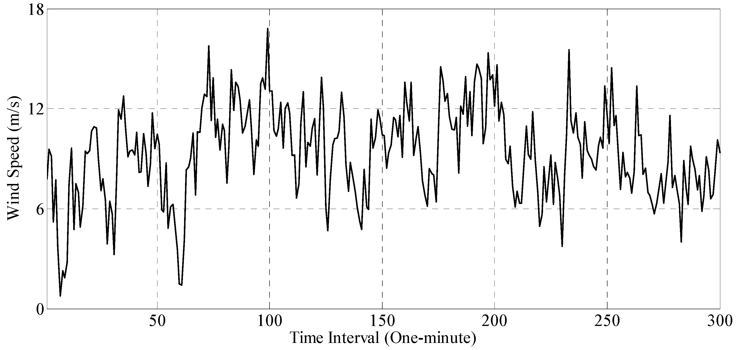
In order to illustrate the performance of the traditional decomposition-based forecasting methods, wind speed data measured by an ultrasonic anemometer the along one of the high-speed rail lines in China are employed as the experimental data. According to [16], sampling with a one-minute time interval is enough for the wind speed time series in high-speed rail wind warning systems. On this basis, the measured wind speed data with continuous 5 h records in 2014 are used where the sampling time interval still adopts a one-minute interval, and thus a total of 300 wind speed data points are contained in the experimental data. Among them, the first 225 data points are used as the initial training data for model training, while the later 75 data points are used as the testing data for model performance evaluation. Figure 2 presents the details of the experimental data in a visual way and these data may have a weak nonstationary characteristic. Table 1 gives the statistical features of these data. From the table, it can be seen that these statistical features of all the original data and the training data are similar, and are slightly different from those of the testing data. Their differences may contribute to reflecting the performance of traditional decomposition-based forecasting methods.

3.3. Performance Comparison of Traditional Decomposition-Based Forecasting Methods

Based on the experimental wind speed data (see in Figure 2), the above two traditional decomposition-based forecasting methods (i.e., a hybrid of one-time DWT decomposition and CKDE, and a hybrid of real-time DWT decomposition and CKDE) are used to perform short-term wind speed predictions. Taking one-step ahead prediction as an example, the impact of the decomposition level number on forecasting accuracy is preliminarily analyzed, where the number of decomposition levels changes from 3 to 11. The results show that the optimal numbers of decomposition levels for the one-time decomposition-based forecasting method and real-time decomposition-based forecasting method were 8 and 9, respectively.
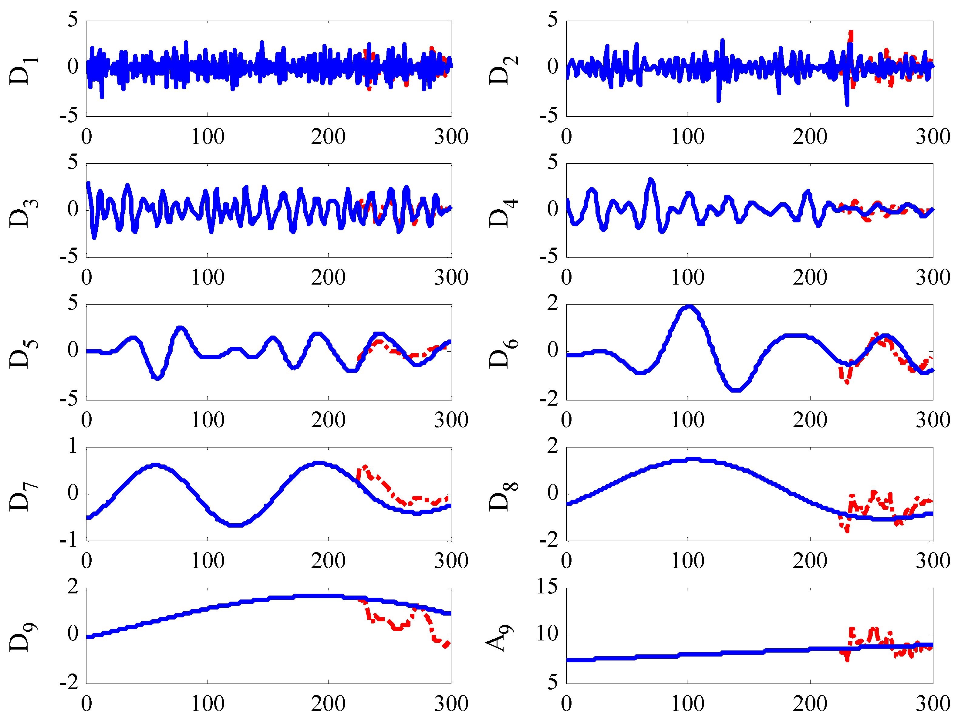
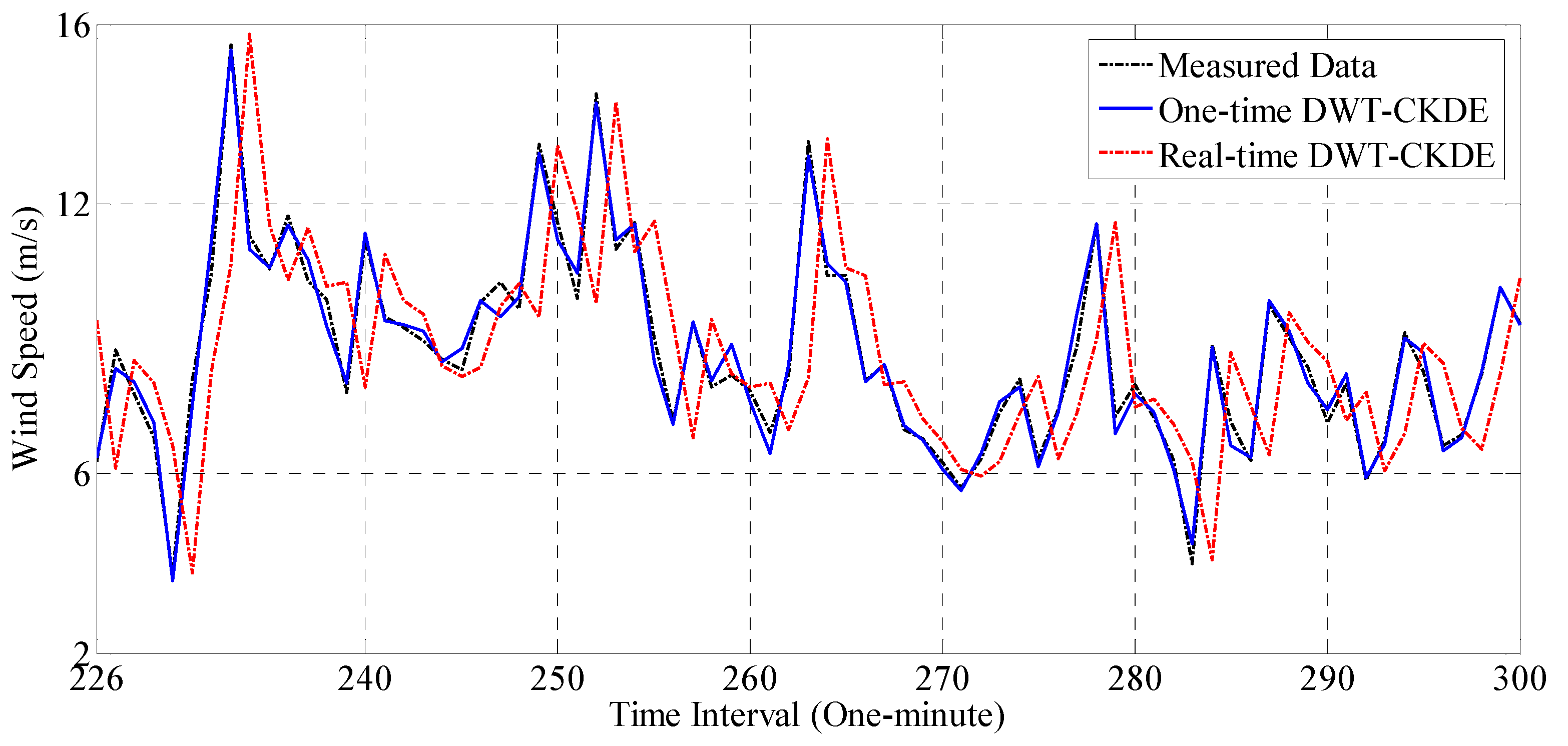
Figure 3 gives the decomposed results with two different decomposition schemes, where the number of decomposition levels is nine. In the figure, the solid line represents the decomposition in the one-time decomposition scheme for all original data, while the dashed line indicates the decomposition in the real-time scheme for the data in the testing set. Meanwhile, it can be observed that the decomposed results (i.e., the dashed lines in the right quarter) in the real-time decomposition scheme are significantly different from those in the one-time decomposition scheme, especially for the low-frequency items which exhibit stronger volatility than those of the one-time decomposition scheme. Figure 4 shows the forecasting results of these two decomposition-based forecasting methods, where both of them take their correspondingly optimal number of decomposition levels. Table 2 presents the corresponding error analysis results.
From Figure 4 and Table 2, it can be seen that the forecasting results of the one-time decomposition-based forecasting method are almost consistent with the trend of the actual wind speed, with the evaluation indexes of MAE, RMSE, and MRPE being 0.23, 0.30, and 2.78%, respectively. Compared with those indicators for the real-time decomposition-based forecasting method, the one-time decomposition-based forecasting method can realize an approximately 86% improvement in terms of these three indicators. On the surface, this method seems to have high potential. However, the decomposition in the one-time decomposition-based forecasting method takes the changing trend of unknown data into consideration, and thus fails to generate the actual required online prediction.
Fortunately, the real-time decomposition-based forecasting method can provide online prediction because the decomposition in this method takes the real-time pattern. However, its forecasting performance is not very stable, and sometimes even underperforms that of a single method. Table 3 summarizes the performance comparison between the real-time DWT-CKDE method and CKDE. It can be seen that the three error indicators of the former are 1.69, 2.15, and 19.69%, respectively, while those of the latter are 1.56, 2.01, and 18.28%, respectively, i.e., the decomposition brings out an obvious performance degradation. Therefore, in practical situations, the real-time decomposition-based forecasting method may not have an advantage. Although the decomposition scheme reduces the nonstationary and nonlinear characteristics hidden in the data, it may introduce other critical problems, such as strong volatility at the end of subsequences (see Figure 3), interferences of modal mixing and illusive components, which have some adverse effects on the performance of the involved predictor.

4. The Proposed Forecasting Method

This section first illustrates the details of the proposed method, then a numerical example based on the measured data in Figure 2 is conducted to exhibit the performance of this method. Finally, practicality analysis based on the other measured wind speed time series is carried out. The specific illustrations regarding these three parts are presented below.

4.1. Processes of the Proposed Method

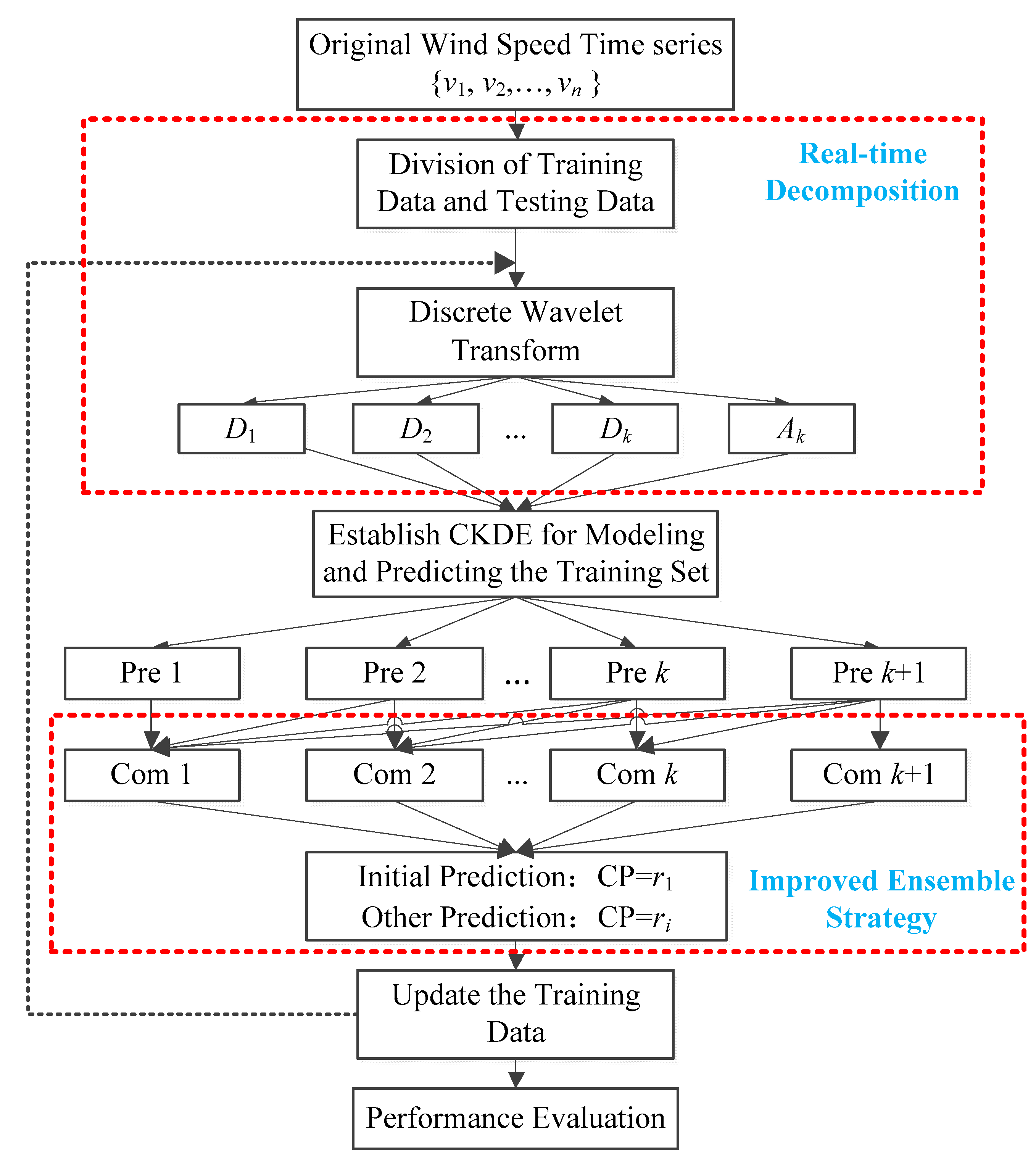
Considering that not all of the decomposed subsequences are beneficial to the overall prediction accuracy of the real-time decomposition-based forecasting method, prediction based on the combination of certain or several subsequence predictions may provide a satisfactory result [20,53]. However, in most existing investigations, the summation of all subsequence predictions in a linear manner is the main ensemble strategy to generate the final prediction, and relevant studies aiming at the ensemble strategy are rarely reported. On this basis, this study explores the combination pattern (CP) of subsequence predictions and develops an improved ensemble-strategy-assisted DWT-CKDE method. This improved ensemble strategy can provide optimization selection for decomposed subsequences for prediction. The specific processes of this developed method are shown in Figure 5, and the corresponding main modeling steps are listed as follows:
(1)
Divide the original wind speed time series v 1 , v 2 , , v n ; n = 300 into an initial training set v 1 , v 2 , , v 225 and a testing set v 226 , v 2 , , v 300 ;
(2)
Perform the DWT decomposition on the initial training samples (the specified number of decomposition levels is set as 9, i.e., k = 8) to obtain the approximation component A k and k detailed components D 1 ,   D 2 ,   ,   D k . Then, the CKDE model is established for training each decomposed subsequence and implementing individual one-step ahead prediction. The predicted values of all subsequences are combined based on the following combination pattern (CP), i.e., D ^ 1 + D ^ 2 + + D ^ k + A ^ k , D ^ 2 + D ^ 3 + + D ^ k + A ^ k , …, D ^ k + A ^ k , A ^ k . On this basis, it is obvious that there k + 1 different CPs (i.e., ensemble strategies) are reserved for ensemble prediction in the next moment (i.e., the result of v ^ 226 ). In above CPs, D ^ j ,   ( j = 1 ,   2 ,   ,   k ) denotes the one-step ahead forecasting value of the detailed component D j and A ^ k stands for the one-step ahead forecasting value of the approximation component A k ;
(3)
When the actual value of v 226 is known, the ideal ensemble strategy (marked as the CP r2) in Step (2) can be identified from k + 1 different CPs based on the minimum absolute deviation criterion, i.e., the prediction based on the ideal ensemble strategy has the smallest deviation with its corresponding actual value;
(4)
Update the training set to v 2 , v 3 , , v 226 (i.e., the known value of v 226 ) and perform the corresponding DWT decomposition where one approximation component A 8 and eight detailed components D 1 ,   D 2 ,   ,   D 8 can be obtained. Then, the CKDE model is established to yield nine individual one-step ahead predictions and nine different CPs. With these predictions and the previous CP r2, the one-step ahead prediction of the wind speed data point v 227 (i.e., the result of v ^ 227 ) can be generated;
(5)
When the actual value of v 227 is known, the ideal ensemble strategy (marked as the CP r3) in Step (3) can also be identified, and it has a similar deterministic process with that of CP r2. This CP r3 provides an ensemble strategy for the forecasting result v ^ 228 ;
(6)
Similarly, update the training set to v i , v i + 1 , , v i + 224 ;   i = 3 ,   4 ,   ,   76 and repeat Step (4) and combine the ensemble strategy CP ri to yield the forecasting result v ^ i + 225 . When the actual value of v i + 225 is known, the ensemble CP ri+1 can be obtained via a similar process with Step (5), which provides an ensemble strategy for the forecasting result v ^ i + 1 + 225 , otherwise the prediction should be terminated. Note that the ideal combination pattern at the previous moment is regarded as the ensemble strategy at the current moment;
(7)
As for the predicted value of v ^ 226 and CP r1, they can be obtained by the following procedures: ① perform the DWT decomposition for the wind speed time series v 1 , v 2 , , v 224 and establish the CKDE model for training and predicting each decomposed subsequence, thereby yielding nine different CPs; ② with the available of the value of v 225 , the ideal ensemble strategy CP r1 can be identified; ③ update the training set to v 1 , v 2 , , v 225 and repeat Step (4), then the predicted value of v ^ 226 can be generated;
(8)
Perform the error analysis based on the performance evaluation indictors given in Section 3.1.
From the above illustration, the proposed method is a hybrid of the real-time DWT decomposition, CKDE, and an improved ensemble strategy. Differing from traditional decomposition-based forecasting methods that generally require all decomposed subsequences involved in the prediction, this method has an ability to take a selective combination of individual predictions. The improved ensemble strategy provides effective guidance for this selective combination with consideration of the historical information in the data. Considering that the updating of training sets may lead to changes in data characteristics and the implied original information of each decomposed subsequence, the ensemble strategy may not be always the same. Therefore, it is necessary to update the combination pattern of the selected individual components in every real-time prediction. This time-varying ensemble strategy and the real-time decomposition scheme may be more beneficial to reflecting the actual complex wind environment.

4.2. Numerical Example

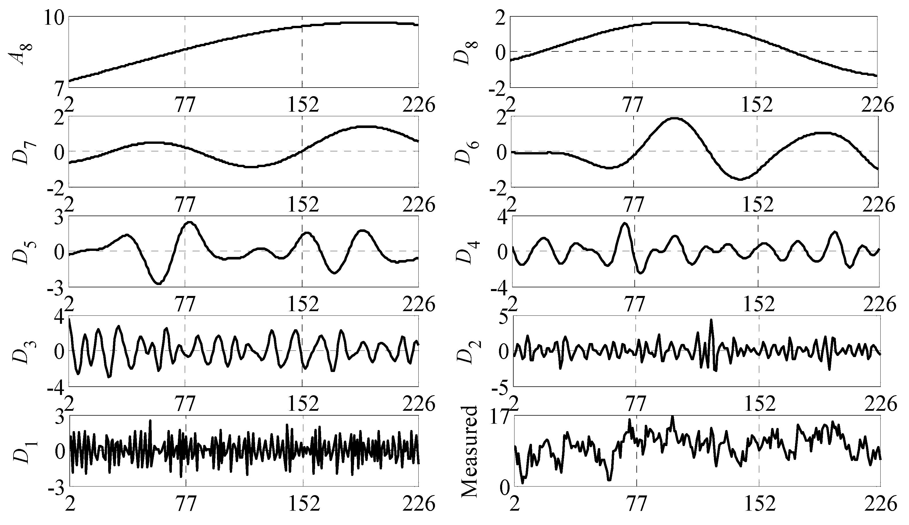
Based on the experimental data in Figure 2, the one-step ahead wind speed prediction is performed. Figure 6 takes the wind speed time series v 2 , v 3 , , v 226 as example to exhibit the decomposed results of DWT. In the figure, it is obvious that the decomposed subsequences are more stationary and regular than the original data. Therefore, the use of DWT to perform the pre-processing operation is effective in reducing the nonstationarity of the original data, which can lay a strong foundation for the application of statistical models, artificial or machine learning models for the prediction. For the sake of exhibiting the effectiveness of the selected combination, Table 4 presents the real-time prediction taking the ideal CP (i.e., each prediction adopts the optimal ensemble strategy which can make the prediction have the smallest deviation from its correspondingly actual value). Meanwhile, the influence of the number of decomposition levels on the forecasting accuracy is also examined. Table 5 gives the comparison of the prediction in the optimal ensemble strategy, real-time DWT-CKDE, and CKDE.
From Table 4 and Table 5, it can be observed that the parameter of k = 8 (i.e., the number of decomposition levels is nine) corresponds to the minimum value of the evaluation indictors, and the prediction in the optimal ensemble strategy presents a higher accuracy than those of the real-time DWT-CKDE method and the CKDE method. For example, the values of three evaluation indicators in terms of the optimal ensemble strategy are 0.73 (MAE), 1.21 (RMSE), and 8.99% (MRPE), respectively. Meanwhile, the corresponding improved degrees of PMAE, PRMSE, and PMRPE in comparison with the real-time DWT-CKDE method are 56.21%, 43.72%, and 54.34, respectively, while those compared with CKDE are 53.21%, 39.80%, and 50.82%, respectively. Obviously, these results demonstrate that the selective ensemble strategy (i.e., the selective combination of several individual predictions) is an effective way to improve the traditional real-time decomposition-based forecasting method. However, due to the lack of selection criteria, it is impossible to obtain an ideal CP in every time prediction.
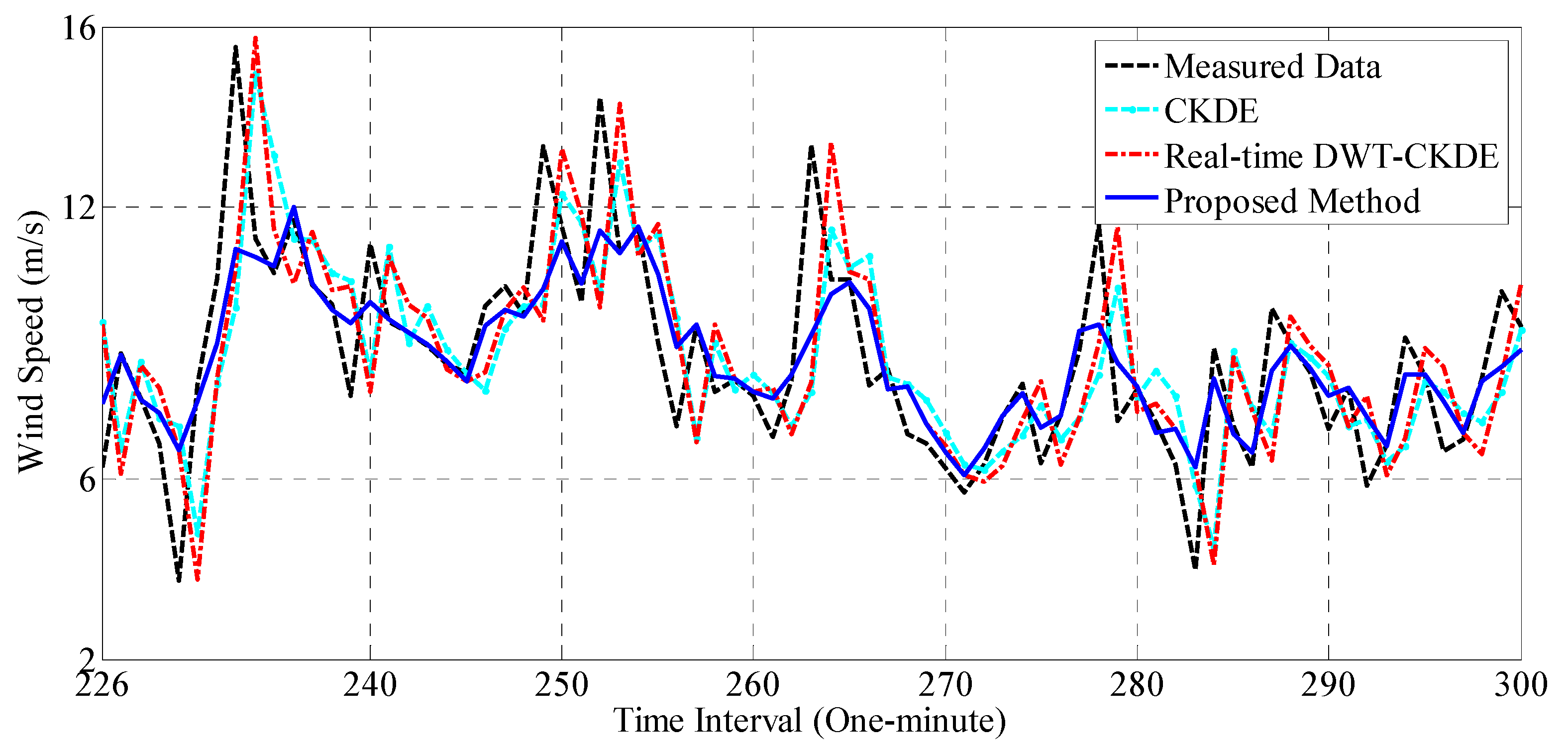
The improved ensemble strategy provides effective guidance to determine the selection criterion. In this strategy, the ideal CP for the previous moment is regarded as the ensemble pattern for the current moment. Table 6 presents all the subsequence predictions D ^ j ,   ( j = 1 ,   2 ,   ,   8 ) and A ^ 8 where the training set is updated to v 2 , v 3 , , v 226 , i.e., the prediction of v ^ 227 . In the table, it can be seen that the idea combination strategy in this moment is D ^ 8 + A ^ 8 (i.e., r3) when the value of v 227 is known, which can be used for the prediction of v ^ 228 . To show the superiority of the proposed method, the real-time DWT-CKDE method and CKDE are used for comparison. Figure 7 intuitively shows the forecasting results of these three methods and the corresponding evaluation indicators are summarized in Table 7. From the figure, it can be seen that there is an apparent time-delaying effect in the prediction, and the proposed method is least affected. Meanwhile, the statistical results in Table 7 also demonstrate that the proposed method outperforms those compared methods. For example, the improved degrees realized by the proposed method in comparison with the real-time DWT-CKDE method regarding the indexes PMAE, PRMSE, and PMRPE are 19.05%, 16.74%, and 16.66%, respectively, while those in comparison with CKDE are 12.82%, 10.95%, and 11.40%, respectively.

4.3. Practicality Analysis

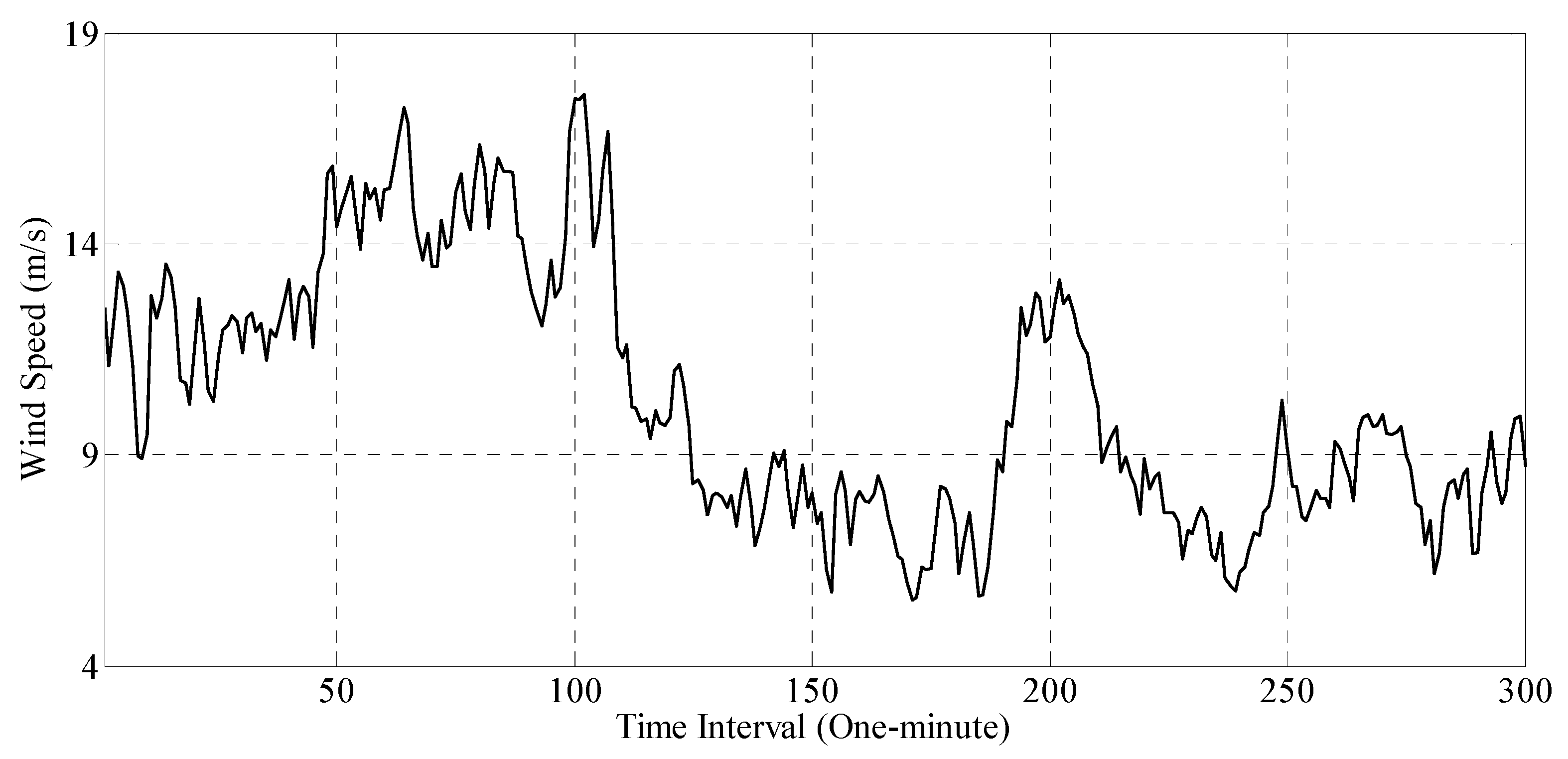
In order to further express the practicability of the proposed method, an additional case study based on the measured wind speed date is performed. Figure 8 and Table 8 give some illustrations regarding the experimental data. From Table 8, it can be seen that the data characteristics in this experiment are significantly different from those in Figure 2 and Table 1. By comparison, these data may have stronger nonstationarity and non-Gaussianity. This difference is conducive to demonstrating the superiority of the proposed method in a more comprehensive way.
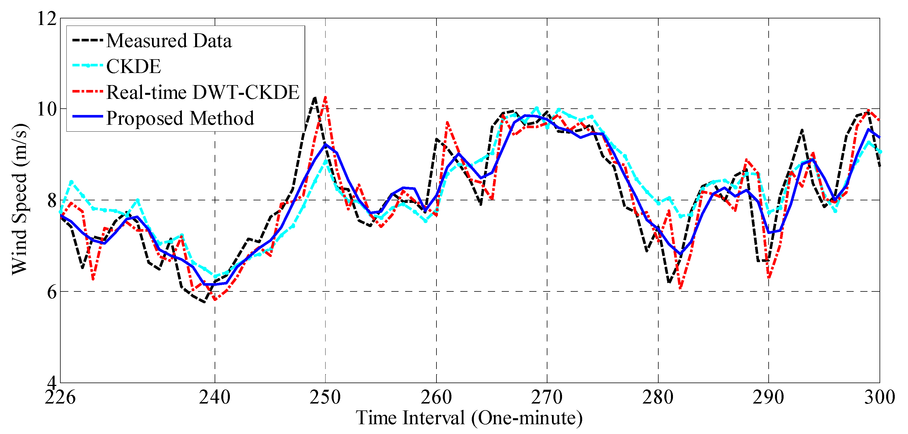
Based on these wind speed data, the one-step ahead prediction is performed, on the basis of which the forecasting performance comparison between CKDE, real-time DWT-CKDE, and the proposed method is also conducted. Figure 9 intuitively presents the forecasting results of these methods, where all of them reflect the main trend of the actual wind speed. By comparison, the proposed method exhibits a higher consistence with the actual wind speed data. Table 9 quantificationally lists the forecasting performance comparison in terms of the evaluation indictors used in this paper. From the table, it can be seen that the proposed method has a higher forecasting accuracy than the other compared methods. For example, the indexes MAE, RMSE, and MRPE of the proposed method are 0.43, 0.54, and 5.38%, respectively, while those of CKDE are 0.54, 0.71, and 6.94%, respectively. Interestingly, in this experiment, the real-time DWT-CKDE method outperforms the single CKDE method, which is the opposite of the corresponding observation in Table 3. The reason for this observation may be ascribed to the advantages of the real-time DWT method (e.g., a good time frequency ability to address nonstationarity and nonlinearity), which contributes more to the forecasting accuracy than the adverse effect of the disadvantages of the real-time DWT on the accuracy (e.g., the adverse impacts of the end effect, modal aliasing, and illusory components).
Computational complexity is another index by which to evaluate the practicality of the model. To this end, Table 10 gives a comparison of the computational costs of all of the involved models in each time prediction, where the time consumption is the average value of 10 operations. From the table, it can be found that the CKDE model generally has the lowest computational cost, while the proposed method possesses the largest time consumption. The reason for this observation is that the proposed method has the highest model complexity. Meanwhile, the difference in computation between one-time DWT-CKDE and real-time DWT-CKDE is very small, indicating that the DWT operation in the experiment takes very little time. Indeed, this time consumption will increase with increases in the amount of wind speed data. In addition, the computational burden of one-time DWT-CKDE is approximately equal to nine times the calculation time of CKDE, i.e., nine different CKDE models are, respectively, established for the corresponding subsequences in the one-time DWT-CKDE.

5. Conclusions

Short-term wind speed prediction is critical for the safe operation of high-speed railways and many methods have been put forward to improve forecasting accuracy. Among them, decomposition-based forecasting methods are widely applied due to their better data processing ability. On this basis, this paper first clarifies the procedures of traditional decomposition-based forecasting methods (i.e., the one-time decomposition-based method and real-time decomposition-based method) as well as their differences based on the commonly used discrete wavelet transform (DWT) and conditional kernel density Estimation (CKDE). To further enhance forecasting accuracy, the paper proposes an improved ensemble-strategy-assisted forecasting method, which is a hybrid of real-time DWT, CKDE, and an improved ensemble strategy. Finally, a numerical example and practicality analysis based on two groups of measured wind speed time series are employed to demonstrate the superiority of the proposed method. Some main observations and conclusions are summarized below.
(1)
The one-time decomposition-based forecasting method has an extremely good forecasting performance. However, this method cannot provide online prediction because the one-time decomposition operation takes future data into consideration.
(2)
The real-time decomposition-based forecasting method can provide online prediction, and thus may have the potential to be implemented in practice. However, the forecasting accuracy of this method is not stable and is sometimes unsatisfactory. Although decomposition methods reduce the nonstationary and nonlinear characteristics of data, they may also greatly increase the volatility of decomposed subsequences (especially for the end part of subsequences), thereby increasing the difficulty of prediction and ultimately leading to poor forecasting results.
(3)
CKDE is still effective in the prediction of short-term wind speeds. This method can be regarded as the nonparametric model to some extent, and thus has a powerful applicability in addressing the time series problem. The numerical case in this paper shows that it even performs better than the decomposition-based forecasting method in some scenarios.
(4)
The combination of several individual predictions (i.e., the prediction of each decomposed subsequence) may have a higher accuracy than the summation of all predictions in the short-term wind speed prediction. Along with this design concept, an improved ensemble strategy is developed which can perform selective combination prediction by analyzing information in the historical data. The experimental results indicate this strategy can clearly improve the forecasting accuracy of real-time decomposition-based methods and the single method. For example, compared with CKDE, the average degrees of improvement realized by the proposed method in terms of MAE, RMSE, and MRPE are 16.25%, 17.66%, and 16.93, respectively, while those in comparison with the traditional real-time DWT-CKDE method are 17.11%, 18.54%, and 16.84, respectively. Therefore, the proposed method may have great potential for railway strong wind warning systems.
Although the proposed method can provide satisfactory forecasting accuracy, it requires the largest computational burden because it possesses the highest model complexity, and its time consumption will increase with increases in the amount of wind speed data. Meanwhile, this method ignores the impact of the inherent limitations of DWT (e.g., the end effect, modal aliasing, illusory components, etc. [19]) on prediction accuracy. In addition, it fails to perform probabilistic prediction, which is critical for risk-orientated decision-making and safety scheduling in high-speed railways.

Author Contributions

Conceptualization, J.L., C.C. and Y.J.; data curation, C.C., J.L., X.C. and Y.J.; formal analysis, J.L., C.C., X.C. and Y.J.; funding acquisition, Y.J.; investigation, J.L., C.C. and X.C.; methodology, C.C. and J.L.; resources, J.L. and Y.J.; software, J.L. and C.C.; supervision, X.C. and C.C.; validation, J.L.; visualization, C.C. and Y.J.; writing—original draft, J.L., C.C., X.C. and Y.J.; writing—review and editing, C.C., J.L., X.C. and Y.J. All authors have read and agreed to the published version of the manuscript.

Funding

This research was funded by “China Postdoctoral Science Foundation (grant number: 2023M730431)”, “Special Funding of Chongqing Postdoctoral Research Project (grant number: 2022CQBSHTB2053)”, “the Science and Technology Research Program of Chongqing Municipal Education Commission (grant number: KJZD-M202300201)”, “State Key Laboratory of Mountain Bridge and Tunnel Engineering (grant number: SKLBT-2202)”, “Chongqing graduate education teaching reform research general project (grant number: YJG233030), “Wind Engineering Research Center of Sichuan Key Laboratory (grant number: WEKLSC202303)” and “the Fundamental Research Funds for the Central Universities (grant number: SWU-KT22021)”.

Institutional Review Board Statement

Not applicable.

Informed Consent Statement

Not applicable.

Data Availability Statement

The data presented in this study are available on request from the corresponding author.

Conflicts of Interest

The authors declare no conflict of interest. Authors Jian Liu and Cheng Cheng are employees of the company Chongqing Wukang Technology Co., LTD. The company had no roles in the design of the study; in the collection, analysis, and interpretation of data; in the writing of the manuscript or in the decision to publish the article. The paper reflects the views of the scientists and not the company.

References

  1. Wang, M.; Wang, X.; Li, X.; Wang, P. Influence of spatial track alignment of long-span arch bridge on train operational stability. Veh. Syst. Dyn. 2023, 61, 3161–3180. [Google Scholar] [CrossRef]
  2. Li, X.; He, H.; Wang, M.; Wang, P. Influence of long-span bridge deformation on driving quality of high-speed trains. Int. J. Rail Transp. 2023, 1–19. [Google Scholar] [CrossRef]
  3. Liu, D.; Wang, T.; Liang, X.; Meng, S.; Zhong, M.; Lu, Z. High-speed train overturning safety under varying wind speed conditions. J. Wind. Eng. Ind. Aerodyn. 2020, 198, 104111. [Google Scholar] [CrossRef]
  4. Yan, N.; Chen, X.; Li, Y. Assessment of overturning risk of high-speed trains in strong crosswinds using spectral analysis approach. J. Wind. Eng. Ind. Aerodyn. 2018, 174, 103–118. [Google Scholar] [CrossRef]
  5. Wang, M.; Chen, X.; Li, X.; Yan, N.; Wang, Y. A frequency domain analysis framework for assessing overturning risk of high-speed trains under crosswind. J. Wind. Eng. Ind. Aerodyn. 2020, 202, 104196. [Google Scholar] [CrossRef]
  6. Chen, R.; Zeng, Q.; Huang, Y.; Xiang, J.; Wen, Y.; Guo, X.; Yin, C.; Dong, H.; Zhao, G. Analysis theory of random energy of train derailment inwind. China Phys. Mech. Astron. 2010, 53, 751–757. [Google Scholar] [CrossRef]
  7. Cheli, F.; Ripamonti, F.; Rocchi, D.; Tomasini, G.I.S.E.L.L.A. Aerodynamic behaviour investigation of the new EMUV250 train to cross wind. J. Wind. Eng. Ind. Aerodyn. 2010, 98, 189–201. [Google Scholar] [CrossRef]
  8. Duan, F.; Song, Y.; Gao, S.; Liu, Y.; Chu, W.; Lu, X.; Liu, Z. Study on Aerodynamic Instability and Galloping Response of Rail Overhead Contact Line Based on Wind Tunnel Tests. IEEE Trans. Veh. Technol. 2023, 72, 7211–7220. [Google Scholar] [CrossRef]
  9. Fang, C.; Li, Y.; Wei, K.; Zhang, J.; Liang, C. Vehicle–bridge coupling dynamic response of sea-crossing railway bridge under correlated wind and wave conditions. Adv. Struct. Eng. 2019, 22, 893–906. [Google Scholar] [CrossRef]
  10. Montenegro, P.A.; Barbosa, D.; Carvalho, H.; Calçada, R. Dynamic effects on a train-bridge system caused by stochastically generated turbulent wind fields. Eng. Struct. 2020, 211, 110430. [Google Scholar] [CrossRef]
  11. Song, Y.; Zhang, M.; Øiseth, O.; Rønnquist, A. Wind deflection analysis of railway catenary under crosswind based on nonlinear finite element model and wind tunnel test. Mech. Mach. Theory 2022, 168, 104608. [Google Scholar] [CrossRef]
  12. Song, Y.; Zhang, M.; Wang, H. A response spectrum analysis of wind deflection in railway overhead contact lines using pseudo-excitation method. IEEE Trans. Veh. Technol. 2021, 70, 1169–1178. [Google Scholar] [CrossRef]
  13. Reis, E.D.; Carvalho, H.; de Oliveira, C.C.; de Vasconcelos, J.A.; Adriano, R.L.D.S.; Lopes, D.C. Geometric Nonlinear Analysis of Self-Supporting Structures for Overhead Transmission Lines. Pract. Period. Struct. Des. Constr. 2023, 28, 04023003. [Google Scholar] [CrossRef]
  14. Aly, A.M.; Chapain, S. Large-scale open-jet testing for cladding design in high-rise buildings: Higher peak pressures compared to wind tunnels. Pract. Period. Struct. Des. Constr. 2022, 27, 04022016. [Google Scholar] [CrossRef]
  15. Arvan, P.A.; Raju, R.D.; Arockiasamy, M. Offshore Wind Turbine Monopile Foundation Systems in Multilayered Soil Strata under Aerodynamic and Hydrodynamic Loads: State-of-the-Art Review. Pract. Period. Struct. Des. Constr. 2023, 28, 03123001. [Google Scholar] [CrossRef]
  16. Liu, H.; Tian, H.Q.; Li, Y.F. An EMD-recursive ARIMA method to predict wind speed for railway strong wind warning system. J. Wind. Eng. Ind. Aerodyn. 2015, 141, 27–38. [Google Scholar] [CrossRef]
  17. Gou, H.; Chen, X.; Bao, Y. A wind hazard warning system for safe and efficient operation of high-speed trains. Autom. Constr. 2021, 132, 103952. [Google Scholar] [CrossRef]
  18. Liu, H.; Liu, C.; He, S.; Chen, J. Short-term strong wind risk prediction for high-speed railway. IEEE Trans. Intell. Transp. Syst. 2021, 22, 4243–4255. [Google Scholar] [CrossRef]
  19. Hoppmann, U.; Koenig, S.; Tielkes, T.; Matschke, G. A short-term strong wind prediction model for railway application: Design and verification. J. Wind. Eng. Ind. Aerodyn. 2002, 90, 1127–1134. [Google Scholar] [CrossRef]
  20. Jiang, Y.; Huang, G. Short-term wind speed prediction: Hybrid of ensemble empirical mode decomposition, feature selection and error correction. Energy Convers. Manag. 2017, 144, 340–350. [Google Scholar] [CrossRef]
  21. Tao, T.; Shi, P.; Wang, H.; Ai, W. Short-term prediction of downburst winds: A double-step modification enhanced approach. J. Wind. Eng. Ind. Aerodyn. 2021, 211, 104561. [Google Scholar] [CrossRef]
  22. Jiang, Y.; Liu, S.; Peng, L.; Zhao, N. A novel wind speed prediction method based on robust local mean decomposition, group method of data handling and conditional kernel density estimation. Energy Convers. Manag. 2019, 200, 112099. [Google Scholar] [CrossRef]
  23. Landberg, L. Short-term prediction of the power production from wind farms. J. Wind. Eng. Ind. Aerodyn. 1999, 80, 207–220. [Google Scholar] [CrossRef]
  24. Yu, C.; Li, Y.; Chen, Q.; Lai, X.; Zhao, L. Matrix-based wavelet transformation embedded in recurrent neural networks for wind speed prediction. Appl. Energy 2022, 324, 119692. [Google Scholar] [CrossRef]
  25. Xin, J.; Jiang, Y.; Zhou, J.; Peng, L.; Liu, S.; Tang, Q. Bridge deformation prediction based on SHM data using improved VMD and conditional KDE. Eng. Struct. 2022, 261, 114285. [Google Scholar] [CrossRef]
  26. Erdem, E.; Shi, J. ARMA based approaches for forecasting the tuple of wind speed and direction. Appl. Energy 2011, 88, 1405–1414. [Google Scholar] [CrossRef]
  27. Jiang, Y.; Liu, S.; Zhao, N.; Xin, J.; Wu, B. Short-term wind speed prediction using time varying filter-based empirical mode decomposition and group method of data handling-based hybrid model. Energy Convers. Manag. 2020, 220, 113076. [Google Scholar] [CrossRef]
  28. Bossanyi, E.A. Short-term wind prediction using Kalman filters. Wind. Eng. 1985, 9, 1–8. [Google Scholar]
  29. Wang, D.; Yang, S.X. Intelligent feature extraction, data fusion and detection of concrete bridge cracks: Current development and challenges. Intell. Robot. 2022, 2, 391–406. [Google Scholar] [CrossRef]
  30. Khasanzoda, N.; Zicmane, I.; Beryozkina, S.; Safaraliev, M.; Sultonov, S.; Kirgizov, A. Regression model for predicting the speed of wind flows for energy needs based on fuzzy logic. Renew. Energy 2022, 191, 723–731. [Google Scholar] [CrossRef]
  31. Zhou, J.; Shi, J.; Li, G. Fine tuning support vector machines for short-term wind speed forecasting. Energy Convers. Manag. 2011, 52, 1990–1998. [Google Scholar] [CrossRef]
  32. Wang, S.; Wang, J.; Lu, H.; Zhao, W. A novel combined model for wind speed prediction–Combination of linear model, shallow neural networks, and deep learning approaches. Energy 2021, 234, 121275. [Google Scholar] [CrossRef]
  33. Lai, L.; Hajirasouliha, I.; Pilakoutas, K.; He, X.; Smyl, D. Applying the Continuous Hidden Markov Model to Structural State Estimation. Pract. Period. Struct. Des. Constr. 2023, 28, 04022073. [Google Scholar] [CrossRef]
  34. Nayak, D.K.; Verma, G.; Dimri, A.; Kumar, R.; Kumar, V. Predicting the Twenty-eight day compressive strength of OPC-and PPC-prepared concrete through hybrid GA-XGB model. Pract. Period. Struct. Des. Constr. 2023, 28, 04023020. [Google Scholar] [CrossRef]
  35. Sun, S.; Cao, Z.; Zhu, H.; Zhao, J. A survey of optimization methods from a machine learning perspective. IEEE Trans. Cybern. 2019, 50, 3668–3681. [Google Scholar] [CrossRef] [PubMed]
  36. Hyndman, R.J.; Bashtannyk, D.M.; Grunwald, G.K. Estimating and visualizing conditional densities. J. Comput. Graph. Stat. 1996, 5, 315–336. [Google Scholar]
  37. Han, Q.; Meng, F.; Hu, T.; Chu, F. Non-parametric hybrid models for wind speed forecasting. Energy Convers. Manag. 2017, 148, 554–568. [Google Scholar] [CrossRef]
  38. Méndez-Gordillo, A.R.; Cadenas, E. Wind speed forecasting by the extraction of the multifractal patterns of time series through the multiplicative cascade technique. Chaos Solitons Fractals 2021, 143, 110592. [Google Scholar] [CrossRef]
  39. Jiang, Y.; Zhao, N.; Peng, L.; Zhao, L.; Liu, M. Simulation of stationary wind field based on adaptive interpolation-enhanced scheme. J. Wind. Eng. Ind. Aerodyn. 2019, 195, 104001. [Google Scholar] [CrossRef]
  40. Liu, M.; Peng, L.; Huang, G.; Yang, Q.; Jiang, Y. Simulation of stationary non-Gaussian multivariate wind pressures using moment-based piecewise Hermite polynomial model. J. Wind. Eng. Ind. Aerodyn. 2020, 196, 104041. [Google Scholar] [CrossRef]
  41. Zhao, N.; Jiang, Y.; Peng, L.; Chen, X. Fast simulation of nonstationary wind velocity fields by proper orthogonal decomposition interpolation. J. Wind. Eng. Ind. Aerodyn. 2021, 219, 104798. [Google Scholar] [CrossRef]
  42. Chen, X.; Jiang, Y.; Zhao, N.; Jia, S.; Wang, X.; Tan, S. Simulation of stationary and nonstationary wind velocity field along a long-span bridge using a numerical truncation method. J. Wind. Eng. Ind. Aerodyn. 2022, 231, 105206. [Google Scholar] [CrossRef]
  43. Li, B.; Peng, L.; Jiang, Y.; Wu, F.; Hui, Y.; Luo, Y. Simulation of stationary non-Gaussian stochastic vector processes using an eigenvalue-based iterative translation approximation method. Mech. Syst. Signal Process. 2022, 175, 109128. [Google Scholar] [CrossRef]
  44. Jiang, Y.; Huang, G.; Yang, Q.; Yan, Z.; Zhang, C. A novel probabilistic wind speed prediction approach using real time refined variational model decomposition and conditional kernel density estimation. Energy Convers. Manag. 2019, 185, 758–773. [Google Scholar] [CrossRef]
  45. Sun, W.; Liu, M. Wind speed forecasting using FEEMD echo state networks with RELM in Hebei, China. Energy Convers. Manag. 2016, 114, 197–208. [Google Scholar] [CrossRef]
  46. Li, Y.; Peng, T.; Zhang, C.; Sun, W.; Hua, L.; Ji, C.; Shahzad, N.M. Multi-step ahead wind speed forecasting approach coupling maximal overlap discrete wavelet transform, improved grey wolf optimization algorithm and long short-term memory. Renew. Energy 2022, 196, 1115–1126. [Google Scholar] [CrossRef]
  47. Meng, A.; Ge, J.; Yin, H.; Chen, S. Wind speed forecasting based on wavelet packet decomposition and artificial neural networks trained by crisscross optimization algorithm. Energy Convers. Manag. 2016, 114, 75–88. [Google Scholar] [CrossRef]
  48. Gilles, J. Empirical wavelet transform. IEEE Trans. Signal Process. 2013, 61, 3999–4010. [Google Scholar] [CrossRef]
  49. Tang, Q.; Jiang, Y.; Xin, J.; Liao, G.; Zhou, J.; Yang, X. A novel method for the recovery of continuous missing data using multivariate variational mode decomposition and fully convolutional networks. Measurement 2023, 220, 113366. [Google Scholar] [CrossRef]
  50. Jiang, Y.; Huang, G.; Peng, X.; Li, Y.; Yang, Q. A novel wind speed prediction method: Hybrid of correlation-aided DWT, LSSVM and GARCH. J. Wind. Eng. Ind. Aerodyn. 2018, 174, 28–38. [Google Scholar] [CrossRef]
  51. Liu, H.; Tian, H.Q.; Li, Y.F. Four wind speed multi-step forecasting models using extreme learning machines and signal decomposing algorithms. Energy Convers. Manag. 2015, 100, 16–22. [Google Scholar] [CrossRef]
  52. Wang, Y.; Wu, L. On practical challenges of decomposition-based hybrid forecasting algorithms for wind speed and solar irradiation. Energy 2016, 112, 208–220. [Google Scholar] [CrossRef]
  53. Guo, Z.; Zhao, W.; Lu, H.; Wang, J. Multi-step forecasting for wind speed using a modified EMD-based artificial neural network model. Renew. Energy 2012, 37, 241–249. [Google Scholar] [CrossRef]
  54. Su, Y.; Huang, G.; Xu, Y.L. Derivation of time-varying mean for non-stationary downburst winds. J. Wind. Eng. Ind. Aerodyn. 2015, 141, 39–48. [Google Scholar] [CrossRef]
  55. Sundararajan, D. Discrete Wavelet Transform: A Signal Processing Approach; John Wiley & Sons: Hoboken, NJ, USA, 2016. [Google Scholar]
  56. Huang, G.; Su, Y.; Kareem, A.; Liao, H. Time-frequency analysis of nonstationary process based on multivariate empirical mode decomposition. J. Eng. Mech. 2016, 142, 04015065. [Google Scholar] [CrossRef]
  57. Liu, S.; Luo, Y.; Peng, L.; Jiang, Y.; Meng, E.; Li, B. Wind pressure field reconstruction based on unbiased conditional kernel density estimation. J. Wind. Eng. Ind. Aerodyn. 2022, 223, 104947. [Google Scholar] [CrossRef]
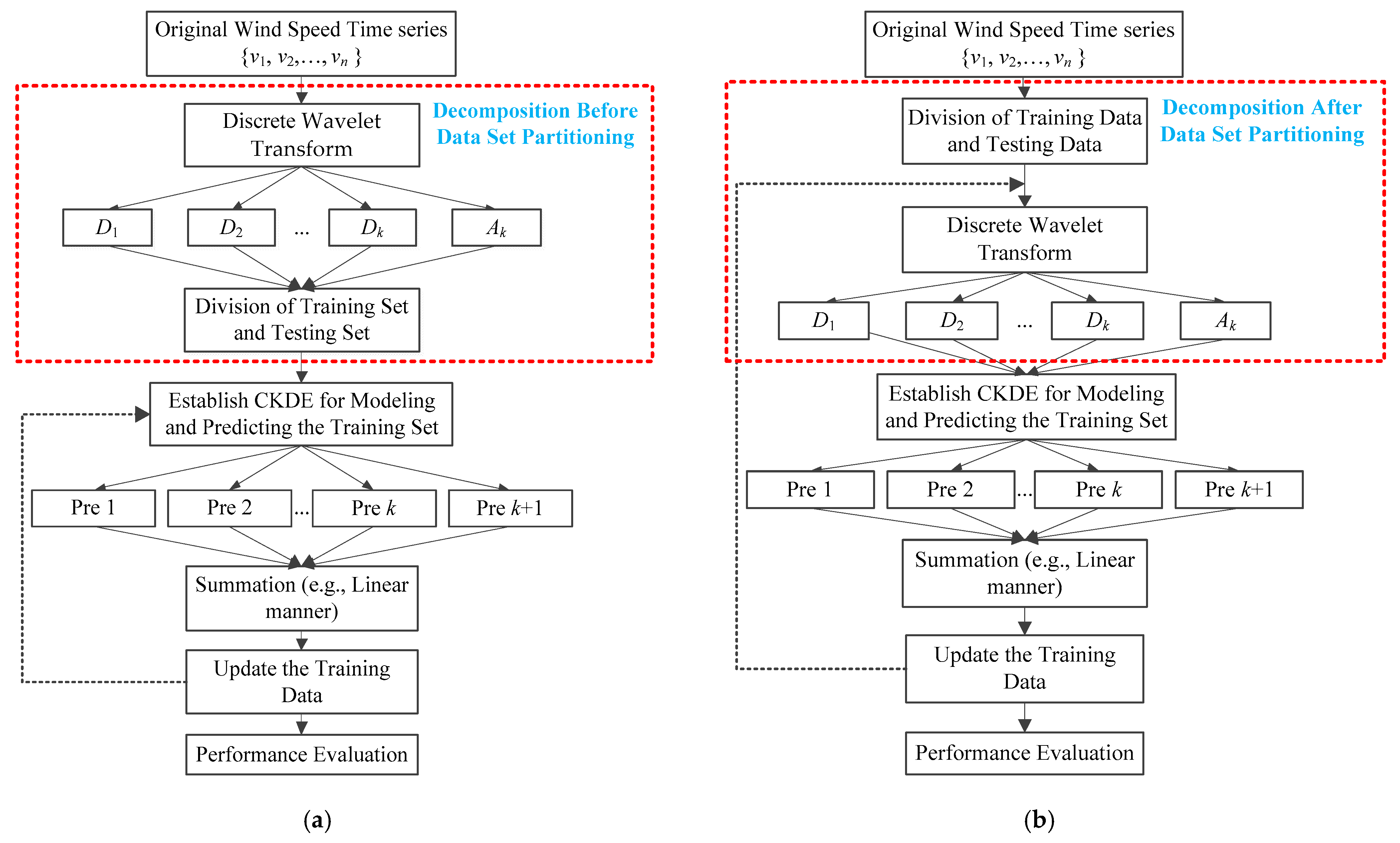
Figure 1. Flowchart of traditional decomposition-based forecasting methods. (a) One-time decomposition-based method. (b) Real-time decomposition-based method.
Atmosphere 14 01787 g001
Figure 2. Original wind speed time series (continuous 5 h records).
Atmosphere 14 01787 g002
Figure 3. Subsequences from one-time decomposition (blue) and real-time decomposition (red).
Atmosphere 14 01787 g003
Figure 4. Forecasting results of the two traditional DWT-CKDE methods.
Atmosphere 14 01787 g004
Figure 5. Flowchart of the proposed model.
Atmosphere 14 01787 g005
Figure 6. Decomposed subsequences of the wind speed time series v 2 , v 3 , , v 226 .
Atmosphere 14 01787 g006
Figure 7. Forecasting results of the proposed model, real-time DWT-CKDE, and CKDE.
Atmosphere 14 01787 g007
Figure 8. Original wind speed time series (additional case).
Atmosphere 14 01787 g008
Figure 9. Forecasting results of the proposed model, real-time DWT-CKDE, and CKDE.
Atmosphere 14 01787 g009
Table 1. Statistical analysis of the experimental wind speed data.
StatisticsMean (m/s)Standard Deviation (m/s)Maximum (m/s)Minimum (m/s)SkewnessKurtosis
All Original Data9.332.7916.820.76−0.223.10
Training Data9.542.9416.820.76−0.483.09
Testing Data8.692.1715.543.740.633.89
Table 2. Comparison of the two traditional DWT-CKDE methods.
Error IndicatorsOne-Time DWT-CKDEReal-Time DWT-CKDEAbsolute Error
MAE0.231.691.46
RMSE0.302.151.85
MRPE/%2.7819.6916.91
Table 3. Comparison of the real-time DWT-CKDE method and CKDE.
Error IndicatorCKDEReal-Time DWT-CKDEAbsolute ErrorPMAE, PRMSE, PMRPE
MAE1.561.69−0.13−7.69%
RMSE2.012.15−0.14−6.51%
MRPE/%18.2819.69−1.41−7.16%
Table 4. Forecasting results by the ideal CP considering the effect of decomposition level number.
Error Indicator34567891011
MAE1.051.000.950.870.840.770.730.780.86
RMSE1.521.471.411.351.321.231.211.241.37
MRPE/%12.5211.9011.3010.4110.109.378.999.2110.19
Table 5. Performance comparison of the ideal CP, CKDE, and real-time DWT-CKDE.
Error IndicatorIdeal EnsembleCKDEReal-Time DWT-CKDE
ResultAbsolute ErrorImproved DegreeResultAbsolute ErrorImproved Degree
MAE0.731.560.8353.21%1.690.9556.21%
RMSE1.212.010.8039.80%2.150.9443.72%
MRPE/%8.9918.289.2950.82%19.6910.7054.34%
Table 6. Forecasting results of all decomposed subsequences and the ideal CP.
Subsequences D ^ 1 D ^ 2 D ^ 3 D ^ 4 D ^ 5 D ^ 6 D ^ 7 D ^ 8 A ^ 8 True   Value   v 227
Prediction−0.690.55−0.19−1.85−0.810.531.18−1.069.708.76 m/s
Ideal CP D ^ 8 + A ^ 8 = 8.64 m/s
Table 7. Performance comparison of the proposed method, CKDE, and real-time DWT-CKDE.
Error IndicatorProposed MethodCKDEReal-Time DWT-CKDE
ResultAbsolute Error Improved DegreeResultAbsolute ErrorImproved Degree
MAE1.361.560.2012.82%1.680.3219.05%
RMSE1.792.010.2210.95%2.150.3616.74%
MRPE/%16.4118.281.8711.40%19.693.2816.66%
Table 8. Statistical analysis of the additional wind speed data.
StatisticsMean (m/s)Standard Deviation (m/s)Maximum (m/s)Minimum (m/s)SkewnessKurtosis
All Original Data10.343.0217.545.550.502.17
Training Data11.103.0817.545.550.121.94
Testing Data8.091.1610.285.7702.10
Table 9. Performance comparison of the proposed method, CKDE, and real-time DWT-CKDE.
Error IndicatorProposed MethodCKDEReal-Time DWT-CKDE
ResultAbsolute Error Improved DegreeResultAbsolute ErrorImproved Degree
MAE0.430.540.1119.67%0.510.0815.17%
RMSE0.540.710.1724.36%0.680.1420.33%
MRPE/%5.386.941.5622.46%6.481.1017.01%
Table 10. Performance comparison of the proposed method, CKDE, and real-time DWT-CKDE.
MethodsOne-Time DWT-CKDEReal-Time DWT-CKDECKDEProposed
Time (s)4.724.800.524.95
Disclaimer/Publisher’s Note: The statements, opinions and data contained in all publications are solely those of the individual author(s) and contributor(s) and not of MDPI and/or the editor(s). MDPI and/or the editor(s) disclaim responsibility for any injury to people or property resulting from any ideas, methods, instructions or products referred to in the content.