A Neural-Network Based MPAS—Shallow Water Model and Its 4D-Var Data Assimilation System

Abstract

The technique of machine learning has been increasingly applied in numerical weather predictions. The aim of this study is to explore the application of a neural network in data assimilation by making use of the convenience in obtaining the tangent linear and adjoint (TL/AD) of a neural network (NN) and formulating a NN-based four-dimensional variational (4D-Var) DA system. A NN-based shallow water (SW) model is developed in this study. The NN model consists of three layers. The weights and biases in the NN-based SW model are trained with 60 years of hourly ERA5 geopotentials and wind field at 500 hPa as initial conditions and the corresponding 12-h forecasts by Model for Prediction Across Scales (MPAS)-SW, in total of 534,697 sets of samples. The 12-h forecasts from independent dates made by NN-based SW prove to closely emulate the simulations by the actual MPAS-SW model. This study further shows that the TL/AD of an NN model can be easily developed and validated. The ease of obtaining the TL/AD makes NN conveniently applicable in various aspects within a data assimilation (DA) system. To demonstrate such, a continuous 4D-Var DA system is also developed with the forward NN and its adjoint. To demonstrate the functionality of the NN-based 4D-Var DA system, the results from a higher resolution simulation will be treated as observations and assimilated to analyze the low resolution initial conditions. The forecasts starting from the analyzed initial conditions will be compared with those without assimilation to demonstrate improvements.

1. Introduction

Forecasts of future atmospheric state has mainly been accomplished by numerical weather predictions (NWP), which is a technology and capability after five decades of development and improvement [1]. Data assimilation (DA) further promoted the capability of NWP to more accurately predict future weather, which is achieved by better capturing initial conditions for NWP and quantifying its uncertainties [2]. In recent years, machine learning (ML), especially neural networks (NN), has been increasingly applied in the atmospheric sciences and has shown great potential [3,4,5,6]. Its capability of recognizing patterns in high-dimensional data sets without needing underlying theoretical equations has been appealing and has benefited various research disciplines [7,8].

Various previous studies have applied ML to NWP. One area is postprocessing NWP model outputs to reduce systematic biases. Ref. [9] used logistic regression and random forests to calibrate the probabilistic precipitation forecasts and improve verification statistics. Ref. [10] applied machine learning to postprocess NWP outputs in high-impact weather events to further improve the forecast skill. Ref. [11] trained a nonlinear NN to predict physical variables such as 2 m temperatures and achieved significant improvement compared to conventional postprocessing methods. Ref. [12] applied deep learning in precipitation nowcasting and 1-hour predictions from radar images. In [13], a deep NN was trained with ensemble weather forecasts for postprocssing, which achieved a relative improvement in ensemble forecast skill of over 14%. Ref. [3] developed a global prediction model using a Fourier Forecasting Neural Network that takes the atmospheric state in the initial conditions and predicts a few 2D variable in future times. Ref. [14] proposed a deep neural network in the form of Graph Neural Network (GNN) [15] to make forecasts in six-hour increments and trained with ERA5 dataset. The forecast performance was shown to outperform the global high resolution operational product, HRES, by the European Centre for Medium-Range Weather Forecasts.

Hybrid modeling combining ML and NWP has also been explored in numerous recent studies. Ref. [16] investigated the possibility of replacing the longwave radiative transfer model with a NN-based model and achieved an accuracy comparable to the conventional algorithm in a general circulation model. Ref. [17] emulated the longwave radiation parameterization for the National Center for Atmospheric Research (NCAR) Community Atmospheric Model with a NN and produced almost identical results 50–80 times faster. Ref. [18] trained a deep neural network to resolve atmospheric subgrid processes in climate modeling by learning from a multiscale model with explicit convections. As promising as the results in these studies show, Ref. [19] pointed out that in hybrid modeling, the feedback between the NN and the General Circulation Model (GCM) can cause instability in simulations and make the experiment crash within days. Similarly, hybrid approaches in DA have been explored in a few studies. Ref. [20] emulated the nonorographic gravity wave drag parametrization with a NN and developed the corresponding tangent linear and adjoint components, which were successfully used in a 4D-Var DA system. Ref. [21] formulated a Lorenz96 model emulator with a NN, generated its Jacobians using the emulator, and applied them in the contexts of 4D-Var DA.

In this study, we develop a feedforward NN [22] with an input layer, one hidden layer, and the output layer to emulate the global shallow water (SW) dynamics in the Model for Prediction Across Scales (MPAS) framework. We train the model on fluid heights and winds from real atmospheric states and then developed the tangent linear and adjoint models of the trained neural network to formulate a continuous 4D-Var DA system, which are described in details in Section 2. The performance in analyzing initial conditions of this DA system as well as the forecast improvements are examined and shown in Section 3. Finally, Section 4 summarizes the study.

2. Methodology

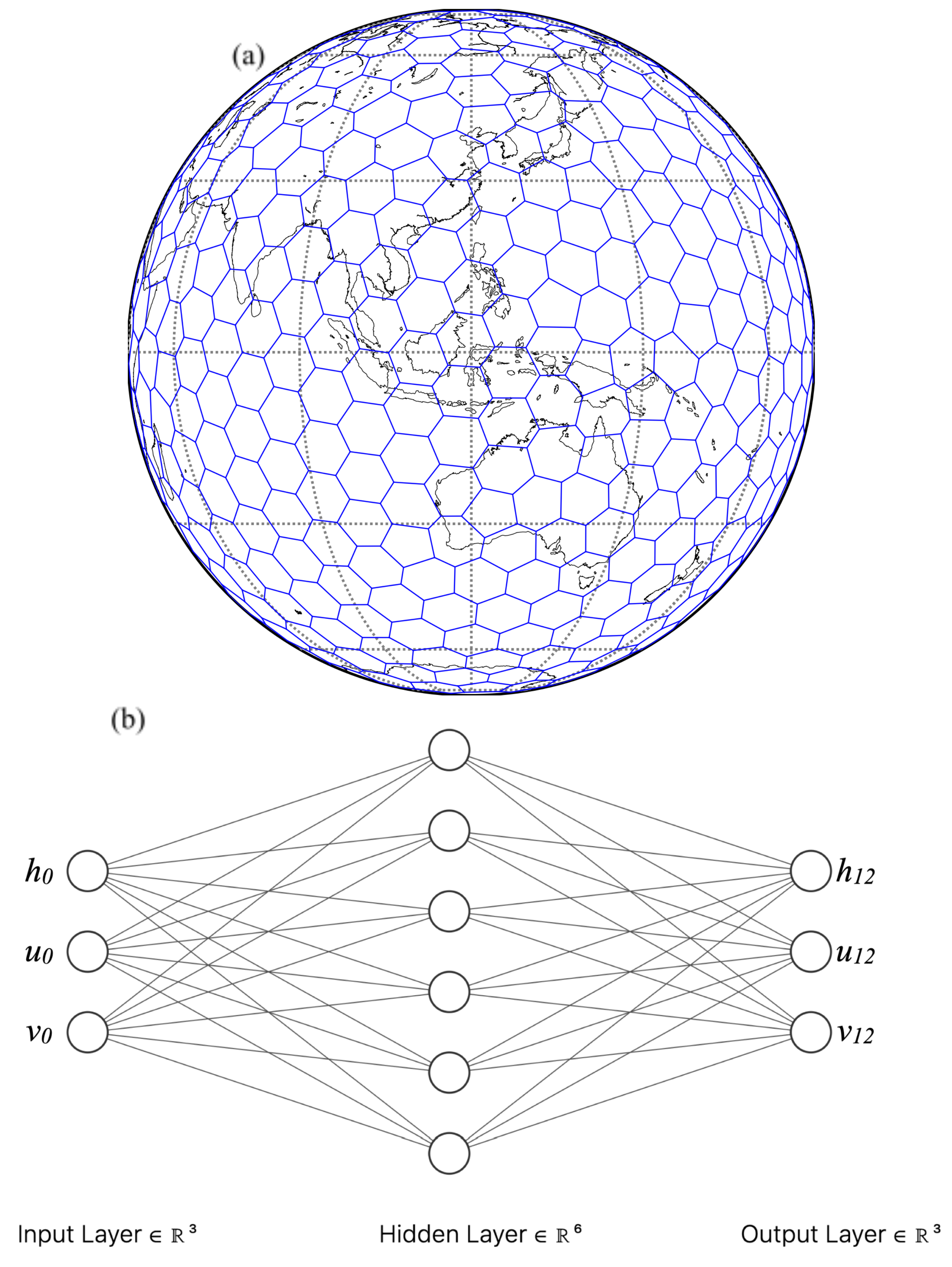
2.1. MPAS-SW Dynamics

The SW dynamics under the MPAS spherical centroidal Voronoi tessellation (SCVT) was developed in [23,24]. The forward nonlinear continuous SW dynamics can be written as:

$$\frac{\partial h}{\partial t}+\nabla \left(h\mathbf{u}\right)=0,$$

(1)

$$\frac{\partial \mathbf{u}}{\partial t}+(\mathbf{u}\nabla )\mathbf{u}+f\mathbf{k}\times \mathbf{u}=-g\nabla (h+b)$$

(2)

where the fluid height h and edge-normal wind $\mathbf{u}$ are the model prognostic variables, f the Coriolis parameter $\theta$ being latitudes, and b the bottom height. This dynamical relationship has been widely applied in meteorology and oceanography. In this study, the height and wind fields at 500 hPa from ERA5 (European Centre for Medium-Range Weather Forecasts Reanalysis v5) [25] will first be interpolated into a 1000 km resolution mesh consisting of 611 cells (shown in Figure 1a) and the MPAS-SW model will make forecasts forward in time.

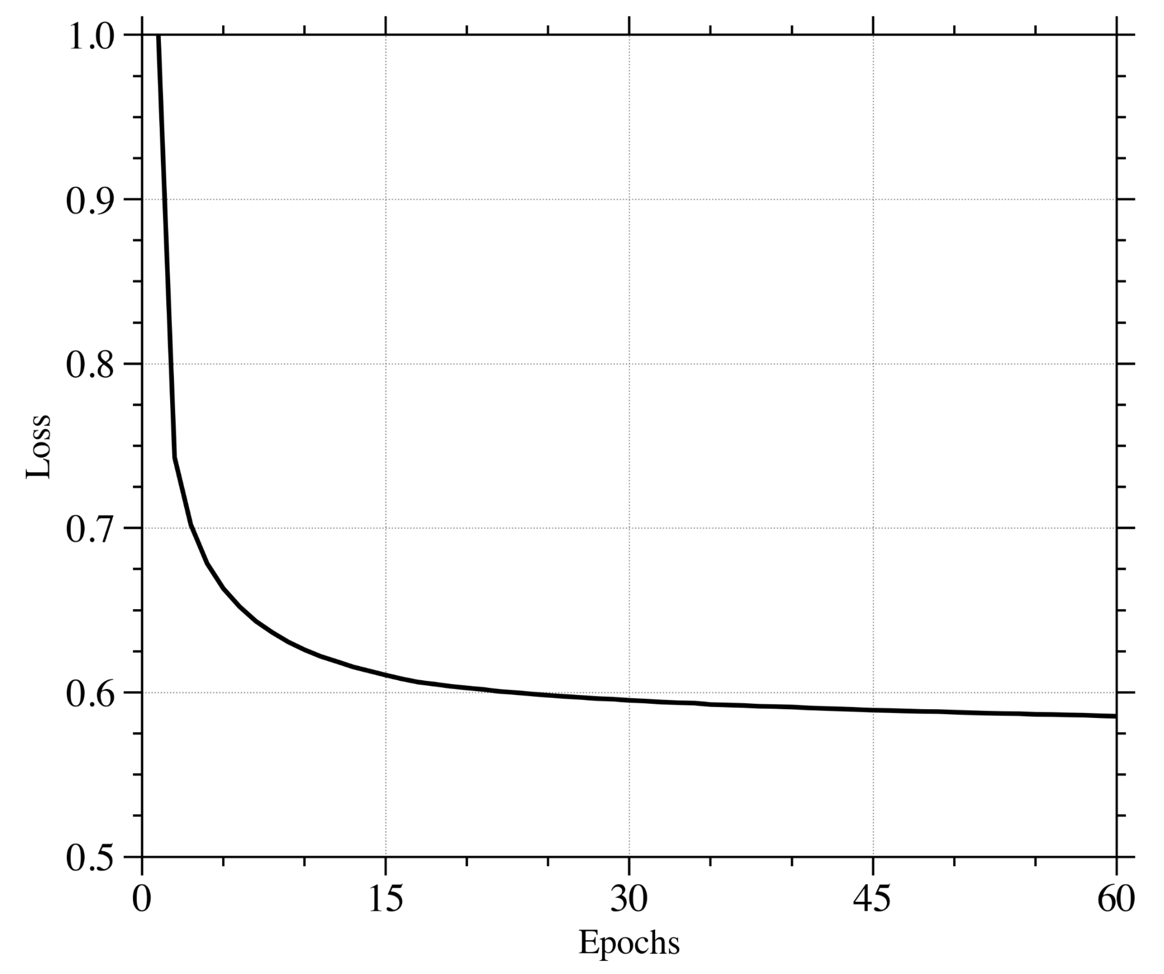
2.2. NN Emulator of MPAS-SW

A feedforward NN is first formulated to emulate the SW dynamical behaviors reflected in MPAS-SW simulations. The atmospheric state in MPAS-SW is essentially represented by vectors. The forecasts are also vectors projected from those from a previous time. Similar to the GNN [15], the benefits of such as representation include intrinsical handling of the global spherical structure of the Earth, allowing to resolve the underlying multiscale interactions between cells, and the potential of learning multiresolution models. Thus, densely connected NN layers are chosen in this study. The NN model consists of three layers: an input layer of 1833 values, a hidden layer with 3666 neurons, and an output layer with 1833 neurons. The input layer holds the three variables including height h, zonal wind velocity u, and meridional wind velocity v over the global domain in the initial condition, all three of which are sampledat the 611 cell centers in the mesh shown in Figure 1a. Thus, each layer has 1833 ($611\times 3$) neurons. The output layer of the same 1833 dimension holds the same three variables (h, u, and v) of the 12-h forecast. The number of neurons in the hidden layer, 3666, was determined based on heuristics. The hidden layer had an ELU activation function [26] and 10% dropout [27], where ELU can be denoted as

$$y=\left\{\begin{array}{cc}\alpha (e^x-1)\hfill & \mathrm{if}x\le 0\hfill \\ x\hfill & \mathrm{if}x>0\hfill \end{array}\right.$$

(3)

where $\alpha =1$ in this study, making both ELU and its derivative continuous. The authors also experimented with various other choices of continuous activation functions including identity, tanh, sigmoid, and Sigmoid linear unit. The ELU proves to yield the best performances emulating the shallow water dynamics. The structure of the NN model is illustrated in Figure 1b.

The NN is trained and validated with hourly 500 hPa height h, zonal u, and meridional wind velocities v from the ERA5 dataset over a 60 years (1959–2019) as features and the corresponding 12-h MPAS-SW as targets, totaling 534,697 samples. The training underwent 60 epochs and a learning rate of $3\times {10}^{-4}$ using the Adam optimizer. Training took 0.5 h on 1 NVIDIA T4 GPU.

The variations of the mean square error as the loss function with respect to the epochs is shown in Figure 2. The model was then independently tested on hourly 500 hPa height and wind fields from 2020 and 2021. The root mean squared error (RMSE) compared with the 12-h MPAS-SW forecasts were 6.32 m and 0.58 m/s in height and wind fields, respectively. Taking the 500 hPa atmospheric state at 00 UTC on 1 January 2021 (shown in Figure 3a) as the initial conditions, the 12-hour forecasts rendered by the NN and the MPAS-SW are given in Figure 3b and Figure 3c, respectively. The distribution of the atmospheric wave patterns from the NN visually resembles the MPAS-SW result to some extent. To further demonstrate the NN emulation of SW dynamics, Figure 4 shows the the differences between the 12-h forecasts and the initial conditions in the case of NN (Figure 4a) and MPAS-SW (Figure 4b). It can be seen that most of the variations in the 12-h forecasts from the initial conditions are captured in the NN results when compared with the actual MPAS-SW simulations.

2.3. The Tangent Linear and Adjoint Models

A nonlinear forward forecast model can denoted as:

$$\mathbf{x}\left(t_r\right)=\mathcal{M}\left(\mathbf{x}\left(t_0\right)\right)$$

(4)

It takes the initial model state $\mathbf{x}\left(t_0\right)$ at time $t_0$ as the initial conditions and predicts the model state $\mathbf{x}\left(t_r\right)$ at time $t_r$. The corresponding tangent linear model is then:

$$\Delta \mathbf{x}\left(t_r\right)=\mathbf{M}\left(\mathbf{x}\left(t_0\right)\right)\Delta \mathbf{x}\left(t_0\right)=\frac{\partial \mathit{M}\left(\mathbf{x}\left(t_0\right)\right)}{\partial \mathbf{x}}\Delta \mathbf{x}\left(t_0\right).$$

(5)

The tangent linear model predicts the perturbation distributions forward in time following the nonlinear trajectory given by the nonlinear forward model in Equation (4). The adjoint model is simply the transpose of the tangent linear model as follows [28,29]:

$$\Delta \widehat{\mathbf{x}}\left(t_0\right)={\mathbf{M}}^T\left(\mathbf{x}\right)\Delta \widehat{\mathbf{x}}\left(t_r\right)$$

(6)

The adjoint model simulates backward in time following the nonlinear trajectory and yields the sensitivity distributions in initial conditions at $t_0$ to a user-specified response function at time t where $t>t_0$. In the cases where prediction models simulate complex behaviors, the tangent linear and adjoint models are developed at source code levels line-by-line. When the adjoint model is applied in a 4D-Var data assimilation system, the simulation propagated forward in time by the nonlinear forecast model will first be compared with existent observation at the observation time. The discrepency, as a sensitivy or forcing term, will then be taken by the adjoint model and be propagated backward in time in a dynamically consistent manner to the model initial time to inform how the initial condition should be adjusted so the simulation at the observation time can agree closer to the observation. The same forward-backward implementation will be repeated with multiple iterations until an optimal solution is found, which will be discussed further in the next subsection.

In the case of densely connected neural networks, an individual layer in the forward model can be rewritten as:

$$\mathbf{y}=F(\mathbf{xW}+\mathbf{b})$$

(7)

where $\mathbf{x}$ is the input of the layer, $\mathbf{W}$ and $\mathbf{b}$ the weights and biases resulted from the training, and F denotes activation functions. The tangent linear model in this case becomes:

$$\delta \mathbf{y}=\frac{\partial F}{\partial (\mathbf{xW}+\mathbf{b})}\delta \mathbf{xW}$$

(8)

The adjoint model is then:

$$\delta \widehat{\mathbf{x}}=\delta \widehat{\mathbf{y}}{\mathbf{W}}^T{[\frac{\partial F}{\partial (\mathbf{xW}+b)}]}^T$$

(9)

A multilayer or deep NN is simply a repetition of the described above. In this study, the hidden layer has an ELU activation function and the output layer has a linear activation function, Equations (7)–(9) can be further reduced to:

$$\mathbf{y}=\mathbf{xW}+\mathbf{b}$$

(10)

$$\delta \mathbf{y}=\delta \mathbf{xW}$$

(11)

$$\delta \widehat{\mathbf{x}}=\delta \widehat{\mathbf{y}}{\mathbf{W}}^T$$

(12)

It is to be noted that, when a variational data assimilation system is aimed to be developed, the activation function of choice is preferred to be continuous, such as the ELU defined in Equation (3), as discontinuity (like in the case of Rectified Linear Unit) in activation functions or models in general will make the tangent linear approximation invalid and cause the data assimilation system difficulty or failure to converge when searching for the optimal solution.

2.4. A Continuous 4D-Var DA System

Given the forward and adjoint models, a 4D-Var DA framework can be built to minimize the the following scalar cost function [30,31,32]:

$$\begin{array}{cc}\hfill J& =J_b+J_o\hfill \\ \hfill & =\frac{1}{2}{({\mathbf{x}}_0-{\mathbf{x}}_b)}^T{\mathbf{B}}^{-1}({\mathbf{x}}_0-{\mathbf{x}}_b)\hfill \\ \hfill & +\frac{1}{2}\sum _{r=0}^N{(H_r\left({\mathbf{x}}_r\right)-{\mathbf{y}}_r)}^T{\mathbf{O}}_r^{-1}(H_r\left({\mathbf{x}}_r\right)-{\mathbf{y}}_r),\hfill \end{array}$$

(13)

where ${\mathbf{x}}_0$ is the analysis to be solved for, ${\mathbf{x}}_b$ the first guess, ${\mathbf{y}}_r$ observations available within the assimilation window, ${\mathbf{x}}_r$ the model state advanced by model $\mathcal{M}$ from ${\mathbf{x}}_0$ to observation time $t_r$, and $H_r$ is the observation operator that maps the model state $\mathbf{x}$ at the observation time $t_r$ to the observation space. The matrices $\mathbf{B}$ and $\mathbf{O}$ are the background and observation error covariance matrices, respectively. Essentially, the term $J_b$ measures the discrepency between the analysis and the model background, weighted by the inverse of the background error covariances, and the term $J_o$ the discrepency between the analysis and the observation weighted by the inverse of observation errors. The solved analysis ${\mathbf{x}}_0$ with the minimum of J yields the minimum variance estimate. The gradient of the scalar J with respect to ${\mathbf{x}}_0$ can be obtained following:

$${\nabla }_{{\mathbf{x}}_0}J={\mathbf{B}}^{-1}({\mathbf{x}}_0-{\mathbf{x}}_b)+\sum _{r=0}^N{\mathbf{M}}_r^T{\mathbf{H}}_r^T{\mathbf{O}}_r^{-1}(H_r\left({\mathbf{x}}_r\right)-{\mathbf{y}}_r),$$

(14)

where ${\mathbf{M}}^T$ denotes the adjoint model and ${\mathbf{x}}_r$ is obtained by advancing analysis ${\mathbf{x}}_0$ forward in time to the observation time with the forward model. In the presence of any observations, the correctness of the overall gradient calculation can be validated with the following:

$$\Phi \left(\alpha \right)=\frac{J({\mathbf{x}}_0+\alpha \Delta \mathbf{x})-J\left({\mathbf{x}}_0\right)}{\alpha \Delta {\mathbf{x}}^T\nabla J\left({\mathbf{x}}_0\right)}=1+O\left(\alpha \right),$$

(15)

3. Experiment Design

The forward NN and its adjoint in Section 2.3 are applied into the equations in Section 2.4 describing the 4D-Var DA system. The NN-based 4D-Var DA system is then used to analyze the initial condition. As described in Section 2, the NN-based SW model is trained with MPAS-SW simulation results at 1000 km resolutions. MPAS-SW was run at 250 km resolution initialized with the ERA5 500 hPa atmospheric state at 00 UTC on 1 January 2021. The simulation results at 12 and 24 h will be interpolated into the 1000 km mesh and assimilated as observations to help analyze the initial conditions at the NN native resolutions. The matrices $\mathbf{B}$ and $\mathbf{O}$ are both kept diagonal and assigned with values of RMSE from the test dataset described in Section 2.2. Taking the entire model state (h, u, and v over the globe) as observations, the correctness of the gradient calculation is first checked following Equation (15), the result of which are shown in Figure 5. As the scaling factor decreases in magnitude, the quantity $\Phi \left(\alpha \right)$ linearly approaches unity, as expected, proving the accuracy of the calculated gradient of the cost function with respect to the model state vector $\mathbf{x}$. As the accuracy in gradient calculation is an essential and necessary step to ensure that the 4D-Var DA system will perform as expected, the results in Figure 5 is a reassuring signal for a working DA system.

3.1. A Single Observation Experiment

The value of height at a single location of $[35.{24}^{\circ }$ N, 164.48${}^{\circ }$ W] from the high-resolution simulations 12 h into the forecast is assimilated. The minimum of the cost function was reached after four iterations as shown in Figure 6a. The norm of the gradient decreased by nearly five orders of magnitude, indicating a local minimum. The analysis increment in both heights and winds are plotted in Figure 6b, with the observation location marked as a white cross. It can be seen that an anticyclonic adjustment was generated near the observation location with some additional adjustments away from the observation location due to the gravity wave mode in the SW dynamics. Notice that only the height at the given location is observed and the background error covariance is kept diagonal in this study, both height and wind adjustments are generated in the analyzed solution, demonstrating the flow dependency in 4D-Var solutions. As simple as this experiment is, a single point observation experiment can be a rather straightforward way of showing the function and feasibility of a DA system.

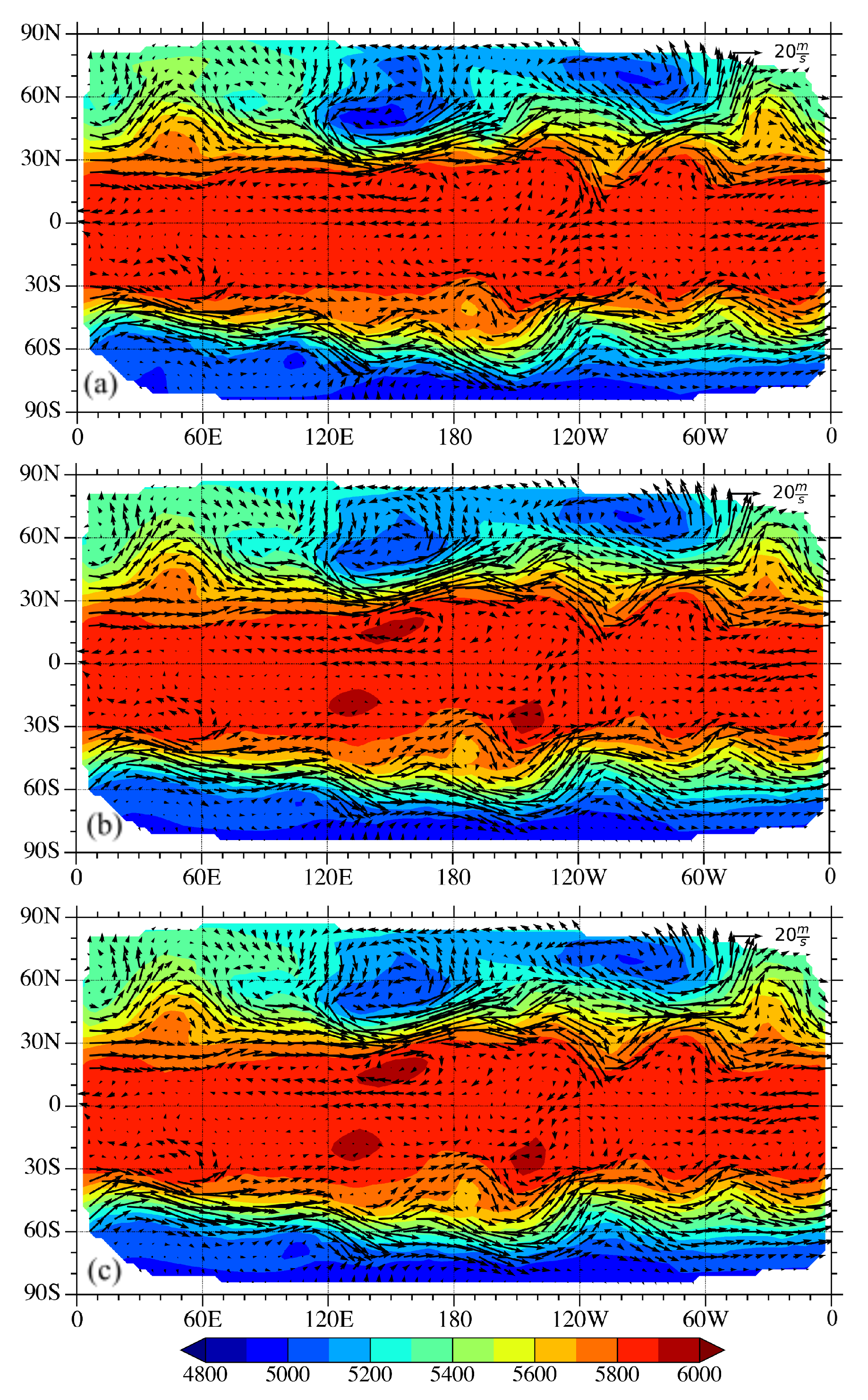
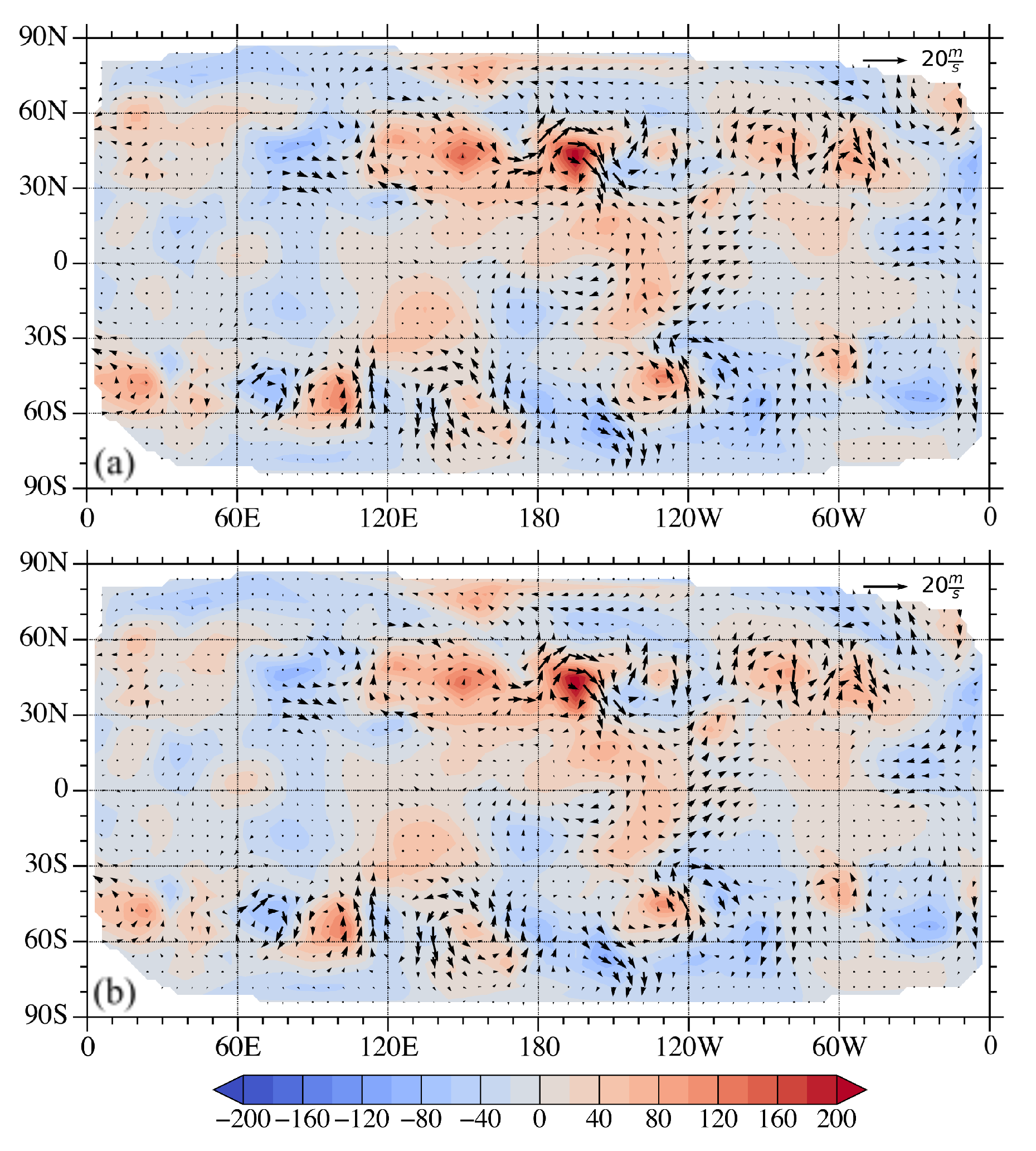
3.2. Full Vector Observation Experiment

The entire atmospheric state (h, u, and v over the global domain) 12 and 24 h after the analysis time simulated by the 250 km resolution MPAS-SW run will be assimilated with the NN-based 4D-Var DA system. The analyzed initial conditions will be used to make forecasts with MPAS-SW at 1000 km resolutions. A control experiment of 1000 km forecast will be made without assimilating any observations, to demonstrate the improvements when observations are assimilated. The predictions with and without DA will be compared against the 250 km simulation results. The evolution of the cost function (solid curve) and the norm of its gradient (dashed curve) are plotted in Figure 7a. After 25 iterations, the value of the gradient norm decreased by more than four orders of magnitude, indicating an extreme point with the solved model state $\mathbf{x}$. The corresponding analysis increment calculated after convergence is given in Figure 7b. Most of the adjustments are located in mid to high latitude regions, especially in the Northern Hemisphere.

Two MPAS-SW simulations at 1000 km are then initialized with the atmospheric state with and without assimilating observations. As the observations come from the 250 km resolution experiment, the 1000 km forecast results from both simulations are compared against the 250 km forecasts in the form of RMSE. Figure 8 shows the differences in RMSE between the control run and that with DA. It shows that in the first four days, the control outperforms the DA experiment when compared with the 250 km simulation results. However, starting from day four, the DA experiment becomes better than the control and this advantage is maintained over 20 days of forecasts. To compare the forecasts from the two experiments spatially, the differences in forecasts between the control and the 250 km simulation are shown in Figure 9a and those between the DA run and the 250 km simulation are shown in Figure 9b. It can be visually seen that the magnitude of differences in Figure 9b is greater than those in Figure 9a, indicating an inferior performance as also illustrated in Figure 8. The same comparison with the 5-day forecasts are shown in Figure 10. In contrast, the magnitude of differences in both heights and winds in the control run are greater than those in the DA experiment, proving forecasts improvements after assimilating observations with the NN-based DA system.

3.3. Discussion

In some of the previous studies, the applications of NN techniques in data assimilation has been explored such as replacing physics parameterization components with a NN [20] or a DA system with Lorenz 96 model [21]. Some studies were even exploring the possibility of scaling ML to the entire NWP system like in [3,14]. This study endeavors to extend the application of NN and make use of the convenience in obtaining the TL/AD of an NN with a global shallow water model to formulate a 4D-Var DA system. The convenience of obtaining the TL/AD from a NN is applicable and can potentially benefit various components in a NWP and DA system demonstrated in the aforementioned studies. One example can be to use NN to approximate certain parts of moist physics parameterizations in the nonlinear forward model, which is a process that often involve nonlinear and/or discontinuous calculations and will make the tangent linear approximation invalid and thus make the 4D-Var technique fail. NN can potentially be useful to emulate the physical process while mitigate the nonlinearity/discontinuity. The tangent linear and adjoint of the physics NN can then be conveniently obtained and more reliably incorporated in a variational DA system. The analyses obtained from the purely NN-based 4D-Var DA prove to improve the forecast performances compared with a control experiment, demonstrating the promising prospect of further applications of NN in DA systems.

The potential next steps for this research are numerous. The NN design in this setup was relatively straight forward since it only had a single hidden layer. Additional hidden layers with more sophisticated NN techniques may be experimented in later studies to produce better emulating results. Similar techniques are readily applicable in substituting moise physics parameterizations or observation operators in a DA system. Furthermore, the analyzed results produced in this study may also be compared with a 4D-Var DA system that needs be developed with the traditional MPAS-SW model adjoint. Finally, applying these techniques to larger models such as the MPAS-Atmosphere model will demonstrate whether these techniques are feasible for NWP operations. The recent advances of ML applications in NWP are especially encouraging in this aspect.

4. Conclusions

This study proposes a NN-based SW model that emulates SW dynamics and makes predictions given an initial condition. The NN-based SW model was trained with 60 years (1959 to 2019) of hourly ERA5 atmospheric state and the corresponding 12-h predictions made with MPAS-SW at 1000 km resolution. Taking the ERA5 atmospheric state in 2020 and 2021 and their MPAS-SW predictions as an independent evaluation, the predictions made with the trained NN have an RMSE value of 6.32 m in fluid heights and 0.58 m/s in wind field. An example of the NN-based prediction result is shown to well capture the atmospheric evolution simulated by shallow water dynamics.

The tangent linear and adjoint models of a NN can be conveniently developed, the process of which is described in this study. The NN-based SW model and its adjoint are used to formulate a continuous 4D-Var DA system. Synthetic observations are made with a MPAS-SW experiment at 250 km resolution that is four times higher than the trained NN native 1000 km resolution. In the presence of observations, the calculation of the gradient of the cost function is checked for correctness to ensure that the minimum of the cost function can be found in the 4D-Var DA system.

In a single point observation experiment, the height value at a single point is assimilated as observation. A convergence is achieved rapidly in five iterations. The analysis increment by differing the analyzed initial conditions from the first guess show both local and remote impacts propagated by gravity waves, indicating flow dependency in the solution, even with a simple diagonal background error covariance. In the second DA experiment, the entire model state vectors, i.e., both height and wind fields over the global domain, 12 and 24 h into the forecasts are assimilated. A convergence was achieved with 25 iterations, in which the norm of the cost function gradient decreased by nearly five orders of magnitude. The analysis increments show adjustments throughout the global domain with greater magnitudes in mid and high latitude regions. Forecasts are created with MPAS-SW at 1000 km initialized with the first guess and the analyzed initial conditions. These forecasts are shown to be closer to the 250 km simulations that served as observations. These encouraging results demonstrate the feasibility of the tangent linear and adjoint components obtained from neural networks and the potential value of the proposed DA system.

References

1. Bauer, P.; Thorpe, A.; Brunet, G. The quiet revolution of numerical weather prediction. Nature 2015, 525, 47–55. [Google Scholar] [CrossRef] [PubMed]
2. Zhang, Z.; Moore, J.C. Mathematical and Physical Fundamentals of Climate Change; Elsevier: Amsterdam, The Netherlands, 2014. [Google Scholar]
3. Pathak, J.; Subramanian, S.; Harrington, P.; Raja, S.; Chattopadhyay, A.; Mardani, M.; Kurth, T.; Hall, D.; Li, Z.; Azizzadenesheli, K. Fourcastnet: A global data-driven high-resolution weather model using adaptive fourier neural operators. arXiv 2022, arXiv:2202.11214. [Google Scholar]
4. Schultz, M.G.; Betancourt, C.; Gong, B.; Kleinert, F.; Langguth, M.; Leufen, L.H.; Mozaffari, A.; Stadtler, S. Can deep learning beat numerical weather prediction? Philos. Trans. R. Soc. A 2021, 379, 20200097. [Google Scholar] [CrossRef] [PubMed]
5. Irrgang, C.; Boers, N.; Sonnewald, M.; Barnes, E.A.; Kadow, C.; Staneva, J.; Saynisch-Wagner, J. Towards neural Earth system modelling by integrating artificial intelligence in Earth system science. Nat. Mach. Intell. 2021, 3, 667–674. [Google Scholar] [CrossRef]
6. Scher, S.; Messori, G. Predicting weather forecast uncertainty with machine learning. Q. J. R. Meteorol. Soc. 2018, 144, 2830–2841. [Google Scholar] [CrossRef]
7. Bildirici, M.; Ersin, O.O. Improving forecasts of GARCH family models with the artificial neural networks: An application to the daily returns in Istanbul Stock Exchange. Expert Syst. Appl. 2009, 36, 7355–7362. [Google Scholar] [CrossRef]
8. Bildirici, M.; Ersin, O. Modeling Markov switching ARMA-GARCH neural networks models and an application to forecasting stock returns. Sci. World J. 2014, 2014, 497941. [Google Scholar] [CrossRef]
9. Gagne, D.J.; McGovern, A.; Xue, M. Machine learning enhancement of storm-scale ensemble probabilistic quantitative precipitation forecasts. Weather Forecast. 2014, 29, 1024–1043. [Google Scholar] [CrossRef] [Green Version]
10. McGovern, A.; Elmore, K.L.; Gagne, D.J.; Haupt, S.E.; Karstens, C.D.; Lagerquist, R.; Smith, T.; Williams, J.K. Using artificial intelligence to improve real-time decision-making for high-impact weather. Bull. Amer. Meteor. Soc. 2017, 98, 2073–2090. [Google Scholar] [CrossRef]
11. Rasp, S.; Lerch, S. Neural networks for postprocessing ensemble weather forecasts. Mon. Weather Rev. 2018, 146, 3885–3900. [Google Scholar] [CrossRef] [Green Version]
12. Agrawal, S.; Barrington, L.; Bromberg, C.; Burge, J.; Gazen, C.; Hickey, J. Machine learning for precipitation nowcasting from radar images. arXiv 2019, arXiv:1912.12132. [Google Scholar]
13. Grönquist, P.; Yao, C.; Ben-Nun, T.; Dryden, N.; Dueben, P.; Li, S.; Hoefler, T. Deep learning for post-processing ensemble weather forecasts. Philos. Trans. R. Soc. A 2021, 379, 20200092. [Google Scholar] [CrossRef] [PubMed]
14. Lam, R.; Sanchez-Gonzalez, A.; Willson, M.; Wirnsberger, P.; Fortunato, M.; Pritzel, A.; Ravuri, S.; Ewalds, T.; Alet, F.; Eaton-Rosen, Z. GraphCast: Learning skillful medium-range global weather forecasting. arXiv 2022, arXiv:2212.12794. [Google Scholar]
15. Keisler, R. GraphCast: Forecasting Global Weather with Graph Neural Networks. arXiv 2022, arXiv:2202.07575. [Google Scholar]
16. Chevallier, F.; Chéruy, F.; Scott, N.A.; Chédin, A. A neural network approach for a fast and accurate computation of a longwave radiative budget. J. Appl. Meteor. Climatol. 1998, 37, 1385–1397. [Google Scholar] [CrossRef]
17. Krasnopolsky, V.M.; Fox-Rabinovitz, M.S.; Chalikov, D.V. New approach to calculation of atmospheric model physics: Accurate and fast neural network emulation of longwave radiation in a climate model. Mon. Weather Rev. 2005, 133, 1370–1383. [Google Scholar] [CrossRef] [Green Version]
18. Rasp, S.; Pritchard, M.S.; Gentine, P. Deep learning to represent subgrid processes in climate models. Proc. Natl. Acad. Sci. USA 2018, 115, 9684–9689. [Google Scholar] [CrossRef] [Green Version]
19. Brenowitz, N.D.; Bretherton, C.S. Spatially extended tests of a neural network parametrization trained by coarse-graining. J. Adv. Model. Earth Syst. 2019, 11, 2728–2744. [Google Scholar] [CrossRef] [Green Version]
20. Hatfield, S.; Chantry, M.; Dueben, P.; Lopez, P.; Geer, A.; Palmer, T. Building Tangent-Linear and Adjoint Models for Data Assimilation With Neural Networks. J. Adv. Model. Earth Syst. 2021, 13, e2021MS002521. [Google Scholar] [CrossRef]
21. Nonnenmacher, M.; Greenberg, D.S. Deep emulators for differentiation, forecasting, and parametrization in Earth science simulators. J. Adv. Model. Earth Syst. 2021, 13, e2021MS002554. [Google Scholar] [CrossRef]
22. Scher, S.; Messori, G. Generalization properties of feed-forward neural networks trained on Lorenz systems. Nonlinear Process. Geophys. 2019, 26, 381–399. [Google Scholar] [CrossRef] [Green Version]
23. Ringler, T.; Ju, L.; Gunzburger, M. A multiresolution method for climate system modeling: Application of spherical centroidal Voronoi tessellations. Ocean Dyn. 2008, 58, 475–498. [Google Scholar] [CrossRef] [Green Version]
24. Ringler, T.D.; Thuburn, J.; Klemp, J.B.; Skamarock, W.C. A unified approach to energy conservation and potential vorticity dynamics for arbitrarily-structured C-grids. J. Comput. Phys. 2010, 229, 3065–3090. [Google Scholar] [CrossRef] [Green Version]
25. Hoffmann, L.; Günther, G.; Li, D.; Stein, O.; Wu, X.; Griessbach, S.; Heng, Y.; Konopka, P.; Müller, R.; Vogel, B. From ERA-Interim to ERA5: The considerable impact of ECMWF’s next-generation reanalysis on Lagrangian transport simulations. Atmos. Chem. Phys. 2019, 19, 3097–3124. [Google Scholar] [CrossRef]
26. Clevert, D.A.; Unterthiner, T.; Hochreiter, S. Fast and Accurate Deep Network Learning by Exponential Linear Units (ELUs). arXiv 2015, arXiv:1511.07289. [Google Scholar] [CrossRef]
27. Srivastava, N.; Hinton, G.; Krizhevsky, A.; Sutskever, I.; Salakhutdinov, R. Dropout: A Simple Way to Prevent Neural Networks from Overfitting. J. Mach. Learn. Res. 2014, 15, 1929–1958. [Google Scholar]
28. Tian, X. Evolutions of Errors in the Global Multiresolution Model for Prediction Across Scales - Shallow Water (MPAS-SW). Q. J. Royal Meteorol. Soc. 2020, 734, 382–391. [Google Scholar] [CrossRef]
29. Tian, X.; Ide, K. Hurricane Predictability Analysis with Singular Vectors in the Multiresolution Global Shallow Water Model. J. Atmos. Sci. 2021, 78, 1259–1273. [Google Scholar] [CrossRef]
30. Zou, X.; Kuo, Y.H.; Guo, Y.R. Assimilation of atmospheric radio refractivity using a nonhydrostatic adjoint model. Mon. Weather Rev. 1995, 123, 2229–2250. [Google Scholar] [CrossRef]
31. Zou, X.; Vandenberghe, F.; Pondeca, M.; Kuo, Y.H. Introduction to Adjoint Techniques and the MM5 Adjoint Modeling System; NCAR Technical Note; NCAR: Boulder, CO, USA, 1997. [Google Scholar]
32. Tian, X.; Zou, X. Validation of a Prototype Global 4D-Var Data Assimilation System for the MPAS-Atmosphere Model. Mon. Weather Rev. 2021, 149, 2803–2817. [Google Scholar] [CrossRef]
Figure 1. (a) Spatial distribution of the Spherical Centroidal Voronoi Tessellation (SCVT) mesh at 1000 km with 611 cells globally. (b) The neural network diagram showing the structure of the NN-based MPAS-SW model. The actual number of the neurons for the input and output layers is N = 1833, and N = 3666 for the hidden layer.
Atmosphere 14 00157 g001
Figure 2. Variations of the loss function with respect to the epochs in the NN training.
Atmosphere 14 00157 g002
Figure 3. (a) The spatial distribution of the fields of height (shaded) and wind (vectors) at 00 UTC 1 January 2021. (b,c) The 12-h forecasts made by (b) the NN-based SW model and (c) MPAS-SW model.
Atmosphere 14 00157 g003
Figure 4. The differences in height (shaded) and wind (vectors) between the 12-h forecasts by (a) NN-based SW and (b) MPAS-SW with respect to the initial conditions.
Atmosphere 14 00157 g004
Figure 5. Variations in the gradient-check results l o g ( | Φ ( α ) 1 | ) as a function of the log of the scaling factor α .
Atmosphere 14 00157 g005
Figure 6. (a) Variation of the cost function (solid curve) and the norm of the gradient (dashed curve) with respect to the number of iterations when assimilating a single point observation. (b) The analysis increment in height (shaded) and wind (vectors) after assimilating only the height at the location marked with a white cross.
Atmosphere 14 00157 g006
Figure 7. (a) Variation of the cost function (solid curve) and the norm of the gradient (dashed curve) with respect to the number of iterations when assimilating the observations of the entire model state. (b) The analysis increment in height (shaded) and wind (vectors).
Atmosphere 14 00157 g007
Figure 8. The differences in root mean squared errors (RMSE) between the control and DA experiments with respect to the forecast lead time.
Atmosphere 14 00157 g008
Figure 9. Differences in 2-day forecasts (a) between the control experiment and referenced high resolution simulations and (b) between the DA experiment and the referenced high-resolution simulations.
Atmosphere 14 00157 g009
Figure 10. Differences in 5-day forecasts (a) between the control experiment and referenced high resolution simulations and (b) between the DA experiment and the referenced high-resolution simulations.
Atmosphere 14 00157 g010
Disclaimer/Publisher’s Note: The statements, opinions and data contained in all publications are solely those of the individual author(s) and contributor(s) and not of MDPI and/or the editor(s). MDPI and/or the editor(s) disclaim responsibility for any injury to people or property resulting from any ideas, methods, instructions or products referred to in the content.