Article

Estimating Site-Specific Wind Speeds Using Gridded Data: A Comparison of Multiple Machine Learning Models

1
School of Atmospheric Sciences, Chengdu University of Information Technology, Chengdu 610103, China
2
Institute of Urban Meteorology (IUM), China Meteorological Administration (CMA), Beijing 100081, China
*
Authors to whom correspondence should be addressed.
Atmosphere 2023, 14(1), 142; https://doi.org/10.3390/atmos14010142
Submission received: 22 December 2022 / Revised: 3 January 2023 / Accepted: 5 January 2023 / Published: 9 January 2023
(This article belongs to the Section Atmospheric Techniques, Instruments, and Modeling)

Abstract

:
Accurate site-specific estimations of surface wind speeds (SWS) would greatly aid clean energy development. The quality of estimation depends on the method of interpolating gridded SWS data to derive the wind speed at a given location. This work uses multiple machine learning (ML) and deep learning (DL) methods to estimate wind speeds at locations across eastern China using the gridded fifth-generation data from the European Centre for Medium-Range Weather Forecasts. The root-mean-square error (RMSE) of these models’ estimates for summer and winter are, respectively, reduced by 23% and 16% on average against simple linear interpolation. A deep convolution neural network (DCNN) consistently performs best among the considered models, reducing the RMSE by 26% and 23% for summer and winter data, respectively. We further examine the dependence of the models’ estimations on altitude, land use category, and local mean SWS. And found that the DCNN can reflect the nonlinear relationships among these variables and SWS. Threfore, it can be used for site-specific wind speed estimates over a large area like eastern China.

1. Introduction

The development of atmospheric models and data assimilation systems has made gridded meteorological data popular, as their wide geographical coverage and long timespans make them convenient for large-scale analyses. As gridded meteorological data represent regional averages within each grid, different horizontal resolutions would mean large differences between the gridded and actual data for a specific site. Current typical reanalysis datasets have a horizontal resolution of 0.25–1°, hindering their direct use in fine analyses.
Surface wind speed (SWS) is a variable that often needs site data that are more accurate than gridded values. For example, site assessment for a prospective wind farm needs accurate, long-term, in situ SWS data [1], outdoor sporting events such as the Winter Olympics are directly affected by the SWS at the location [2], and airports need the wind speed on the runway to ensure aircraft safety [3]. However, the complexities of ground conditions can make SWS vary sharply in the horizontal direction, resulting in significant differences between gridded SWS and in situ observations. Therefore, for a given location without in situ measurements, the gridded SWS data must be mapped to the location by one of a variety of methods. A uniformly applicable grid-to-site conversion scheme will greatly expand the applicability of gridded SWS data.
Interpolation is traditionally used for such conversion. There are various interpolation methods, but most of them, such as kriging, inverse distance weight interpolation, spline interpolation, etc., are mostly used to map discrete variables into a predicted surface [4]. Therefore, these methods are mostly used in meteorology for site-to-grid interpolation calculations. However, in this paper, we choose to interpolate from grid points to sites, so we choose two commonly linear methods (LM), nearest interpolation (NI) and bilinear interpolation (BI) [5,6]. The former directly uses the values for the nearest grid point to a site, whereas the latter performs linear interpolation in each of the east–west and north–south directions. As these linear methods cannot consider factors such as terrain height or land use at a site. They also cannot employ a nonlinear relationship between the grid and site SWS data. Therefore, their estimation accuracy varies sharply grid-by-grid [5,7]. Regression models (RMs), including ridge regression and least absolute shrinkage and selection operator (LASSO) regression, partly overcome the constraints of linear interpolation because they can introduce estimating factors and nonlinearity by adding regularization terms [8,9]. However, such weak nonlinearity cannot reproduce the complex relationship between gridded and site SWS data. Previous studies have reported that linear interpolation and RMs often perform well in regions with generally homogeneous meteorological and land surface conditions but become worse in regions with complex land surface conditions [10,11]. Therefore, a grid-to-site conversion scheme for SWS is required to include more nonlinearities and various factors and to be widely applicable across a large region.
Machine learning (ML) has recently shown strong capabilities for handling nonlinear problems in a variety of fields [12,13]. Compared with traditional linear methods, ML can also conveniently introduce additional factors such as terrain height and land use; it is thus expected to give better interpolation results. For example, some studies have applied various ML models to interpolate data for earthquakes, solar radiation, and sea surface height [14,15,16]. Examples include ML-based missing values filling and resolution downscaling [17,18]. These prior studies all showed that ML improves the interpolation accuracy.
ML has also been used for SWS modeling, but mainly with a focus on forecasting including nowcasts [19,20,21,22], short-range forecasts [23,24,25], and correcting numerical weather prediction models’ outputs for sites [26,27] and grid points [28,29]. Many variables related to SWS are incorporated into ML models to reduce SWS forecasting errors: these include meteorological data (e.g., surface pressure, air temperature, and humidity 2 m above ground level) and static data (e.g., terrain height and land use). Studies of ML-based grid-to-site conversion have focused mainly on small areas and been aimed at SWS data downscaling [30,31]. These studies have used ML methods to statistically downscale wind speeds over the UK, the Korean Peninsula in general, and South Korea specifically. Validation results have demonstrated that this method produces better results compared with any previous statistical method applied to wind resource assessment and that it is comparable to the results of dynamic downscaling.
Some unresolved problems with grid-to-site conversion remain. First, previous studies have considered a single site or small areas, rather than large areas [32]. Although some commonly used ML models, such as random forests (RF), extreme gradient boosting (XGBoost), and various deep learning (DL) models, perform well in small areas [33,34], there is a lack of studies applying them to large areas with complex ground surface conditions, such as China. Second, previous studies have mainly aimed to propose a given model rather than discuss the differences among various ML models, and thus they considered only a few models [35]. Therefore, it is necessary to systematically compare the commonly used ML models in a broad study. Third, owing to the significant differences in meteorological conditions, ML models should be trained separately for different seasons. For example, Liu et al. [29] established models based on RF for grid-to-site conversion in four seasons in the Beijing area and reported better performances in summer and autumn than in spring and winter. The potentially varying seasonal applicability is worth discussing for other commonly used ML models.
Eastern China is influenced by the East Asian monsoon and has continuous and stable wind resources. Therefore, there is high demand for SWS data at potential wind farm sites. We would like to discuss the usability of using machine learning methods for the uniform modeling of wind speed estimation over a large area such as eastern China by taking advantage of the fact that machine learning methods are computationally fast and can handle nonlinear problems. This study investigates grid-to-site conversion models for this region using gridded data from the fifth-generation European Centre for Medium-Range Weather Forecasts global climate reanalysis dataset (ERA5) and 3 h measured wind speed at 10 m above ground level (WS10) from the China National Meteorological Observation Network. We estimate the site WS10 from ERA5 winter and summer data using various ML models, including decision tree (DT), RF, XGBoost, multilayer perceptron (MLP), and DCNN. We compare them with linear interpolation and two RMs, ridge and LASSO. The results show that the ML methods are significantly better than linear interpolation and the RMs, especially for summer data. Among the ML models, XGBoost and DCNN perform best. The effects of altitude, land use category (LUC), and mean WS10 on the performance of these models are also discussed. We find that the DCNN outperforms the other models in estimating data for complex terrain and areas with high wind speed.

2. Data and Methods

2.1. Data and Samples

We use the ERA5 with a horizontal resolution of 0.25° × 0.25° as the input gridded data. Six gridded surface meteorological variables are used to estimate WS10 at the given locations: east–west wind (U10), north–south wind (V10), WS10, air temperature (T2), dew point temperature (D2) at 2 m, and surface pressure (P0). We also introduce two additional quasi-static variables, altitude (H) and LUC (Table S1), owing to their close relationship to WS10 [36,37,38,39,40]. There are 30 LUCs. Unlike the other seven variables, LUC is a discrete variable labeled by number and cannot be input directly. Therefore, we use one-hot encoding to encode it into 30 LUC variables, each corresponding to one category. For an example grid cell with a LUC of water body, the water body variable has a value of 1, and the rest of the LUC variables have a value of 0. The target variable is the site-specific WS10 observations over 2102 basic sites in eastern China (10–60° N, 105–152° E), and the time resolution of 3 h. The data are obtained from the China National Meteorological Observation Network (https://data.cma.cn/, accessed on 20 November 2021.) and are subject to strict quality control [37,41,42].
Linear interpolation uses only the WS10 of the grid points near each site as input variables. The RMs and tree models (TM) have input variables that include all six gridded meteorological variables on a 5 × 5 grid around each site, the two static variables, and the LUC of the grid where the site is located. In addition, the distance between the site and each grid point is added as an input variable to introduce the relative position of the site in the grid. For the DCNN model, the input variables include all 38 variables on a 5 × 5 grid around each site given that the convolution can learn the spatial pattern around the sites.

2.2. Models

We compare nine grid-to-site conversion models for WS10 data (Table 1). The LMs are simple NI and BI, which have shown similar performance for wind speed interpolation [6]. The traditional RMs are ridge regression and LASSO regression. Both models add a regularization term after the loss function of the linear regression, and thus their complexity can be effectively controlled to prevent overfitting [43]. Ridge and LASSO regression use L2 and L1 regularization, respectively. The former has less weight constraint than the latter [44,45]. Weight constraint allows a model to efficiently utilize spatial information, reduce the training time, and improve its estimation accuracy [8,9].
The DT uses a bifurcation structure to fit the target value by traversing all features to determine the optimal decision option [46]. RF and XGBoost are based on DTs, but employ integrated algorithms, i.e., the final estimates are obtained by constructing multiple DTs and integrating all the results for voting. RF uses DTs that are independent of each other and are constructed by randomly sampling the dataset. The final output is obtained using a weighted average of the results obtained from all trees [47]. In the XGBoost models, the DTs are connected in series with each other. The later constructed DTs would fit the residuals of the previous tree to get the final output value by continuously reducing the residuals [48,49]. TMs are widely used for predicting wind speed and revising predictions [50,51].
The DL methods are the MLP and the DCNN. The MLP adds multiple hidden layers between the input and output layers and connects them with nonlinear activation functions [52]. The MLP used here has six hidden layers, the largest having up to 2048 hidden units, and the rectified linear unit (ReLU) as the activation function in each layer. Dropout [53] technology is used to increase the robustness of the model. The DCNN used here follows Zhu et al. [54]. This model is based mainly on DenseNet [55,56], but with the introduction of convolutional block attention modules (CBAM) [57]. Here we use the DCNN with three dense blocks. Each block is connected to the other two using CBAM and transition layers with the 1 × 1 convolution kernel.
We establish uniform modeling instead of point-by-point modeling for all seven non-linear models. This is because unified modeling allows a model to be applied over a large range and quasi-static data (i.e., altitude and LUC) cannot be introduced into a point-by-point model as input variables given a fixed value of these variables at a specified location.In another word, regardless of whether the input grid data are dynamic or static, these models can convert them to wind speeds at the specified site at the corresponding time.
This work uses three metrics to assess the performance of the models. The root-mean-square error (RMSE), mean bias (MB), and the coefficient of determination (R2). The two traditional RMs (Ridge and Lasso) and three TMs (DT, RF, XGBoost) were implemented on the Python platform using the scikit-learn library. The MLP and DCNN were implemented on the Python platform using the Pytorch library.

2.3. Training and Validation

All seven non-linear models use big data for training and validation. Considering the large sample size in this study, we use the leave-out method of validation, which directly divides the data into two mutually exclusive sets, one for training and the other for validation, to reduce the computation time. For summer data, we use values from June, July, and August 2019 and June 2020 for training and those from July 2020 for validation. The winter training data are from December 2019 and January, February, and December 2020; January 2021 data are for validation. The training and validation set contains about 2 million and 0.52 million samples, respectively, for both winter and summer (Table 2). Both RMs select the best regularization coefficients using 10-fold cross-validation. The three DT-based TMs have a maximum depth of 50 layers. The MLP and DCNN are trained over 20 epochs. All these models use the mean-square error as the loss function.
Figures S1 and S2 show scatter plots for the seven models on the training and validation sets in the summer. Ridge regression has an R2 of 0.43, MB of 0.02, and RMSE of 1.26 on the training set. LASSO regression has similar results on the training set (R2 = 0.42, MB = 0.02, and RMSE = 1.27). The performances of both RMs with the validation set are slightly poorer than for the training set, but there is no significant overfitting: R2 = 0.38, MB = 0.06, and RMSE = 1.24.
Compared with the two RMs, the three TMs have fewer errors. The DT has R2 = 0.51, MB = 0.02, and RMSE = 1.17; XGBoost has R2 = 0.59, MB = 0.2, and RMSE = 1.06. The results for DT and XGBoost are also consistent for the training and validation sets, indicating no significant overfitting. In contrast, RF performs very inconsistently on the training and test sets. The R2 and RMSE on the training set are 0.92 and 0.46, respectively, and the corresponding values for the validation set are 0.54 and 1.06, respectively. This inconsistency indicates severe overfitting. Moreover, tuning the hyperparameter cannot reduce the overfitting.
The two DL models perform more consistently than the other models on the training and validation sets. The MLP has R2 values of 0.45 and 0.45, MBs of −0.09 and −0.02, and RMSEs of 1.24 and 1.16, respectively, for the training and validation sets. DCNN shows the best and the most stable performance among all seven models, with R2 values of 0.6 and 0.56, MBs of 0.03 and 0.1, and RMSEs of 1.05 and 1.04, respectively, for the training and validation sets.
Figures S3 and S4 show the seven models’ results for the training and validation datasets for winter. The results are like those for summer: the DCNN outperforms the other models, and RF suffers from overfitting (albeit more severely than for the summer data). The overall RMSEs are slightly larger for winter than for summer. All models except the MLP show overestimation (positive MB) for the winter training set just like summer. For the validation set, all the models except the MLP overestimate WS10 for summer but underestimate it in winter. This is attributable to the magnitude and variability of wind speed being greater in winter than in summer.

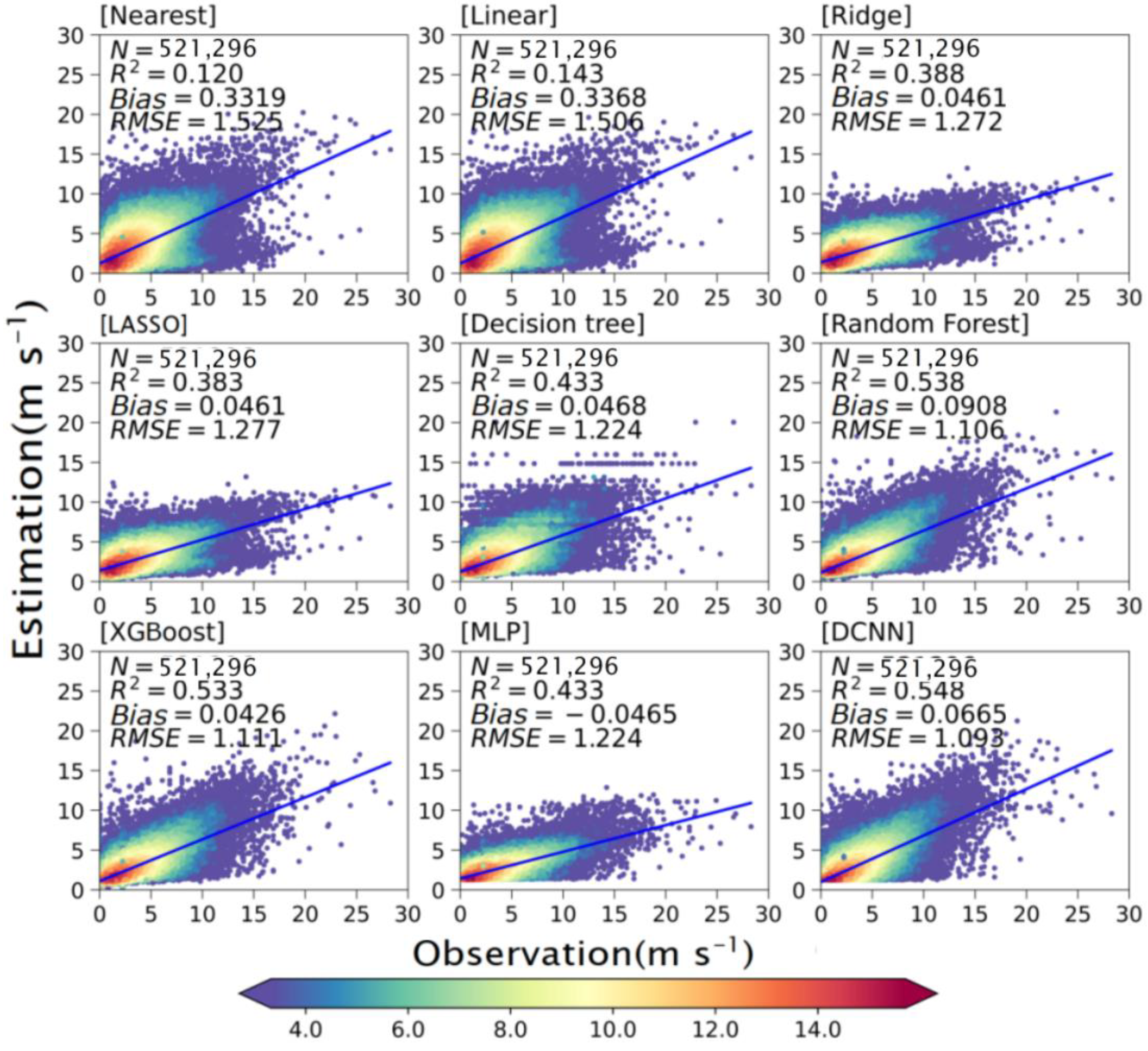
3. Results for the Test Dataset

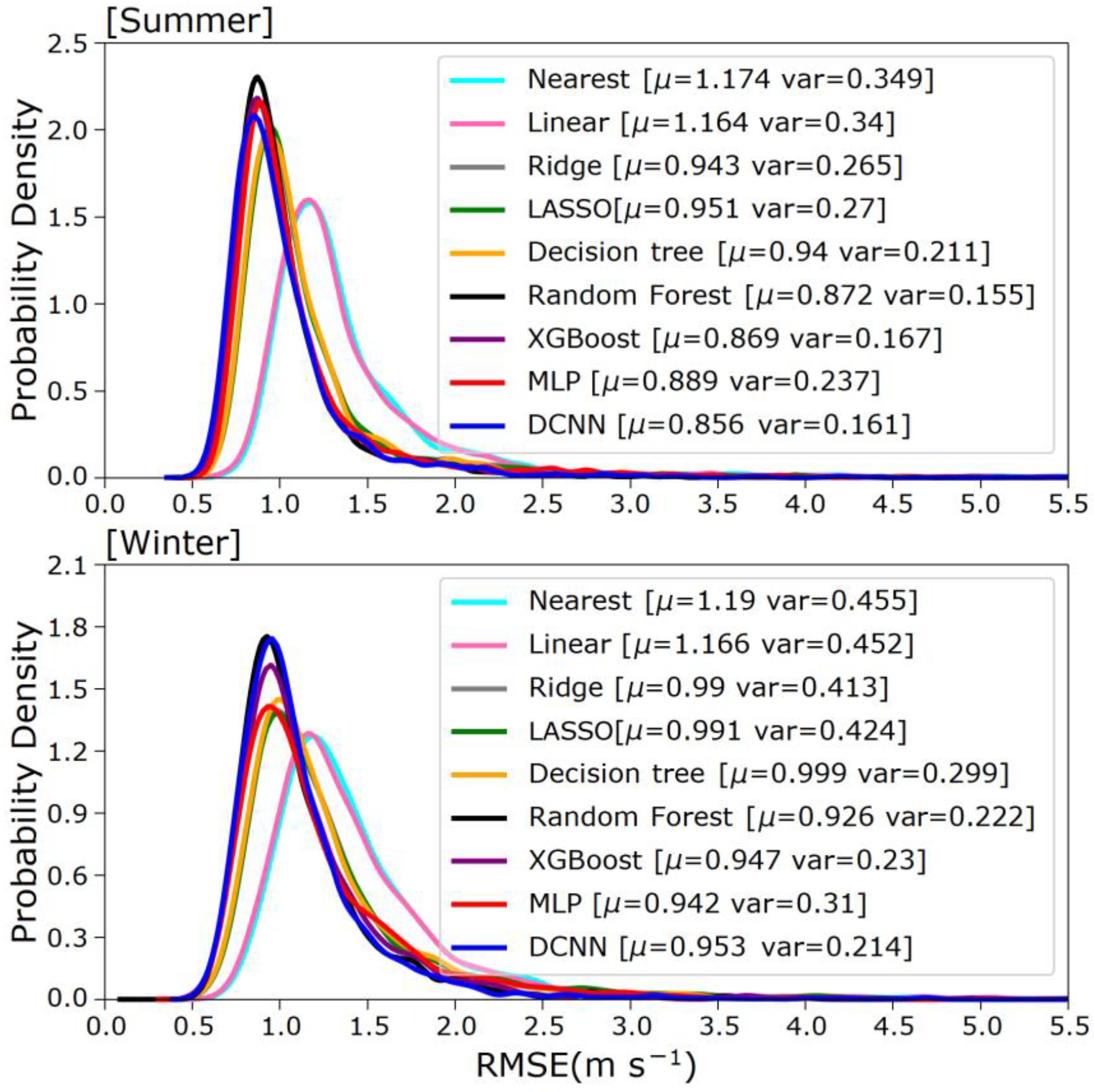
3.1. Regional Averaged Estimation Error

The August 2020 (about 0.52 million samples) and February 2021 (about 0.47 million samples) datasets are the test sets for summer and winter, respectively (Table 2). Figure 1 and Figure 2 show scatter plots of the observations and predictions for all the winter and summer test samples, respectively. For both winter and summer, the RMs have lower errors than the LMs, whereas the DL models and the TMs outperform the RMs. For summer, the DCNN has the highest predictive power among all schemes, with an R2 value of 0.55 and RMSE of 1.09, better than ridge regression (the better regression scheme; R2 = 0.39, RMSE = 1.27) and RF (the best TM; R2 = 0.54, RMSE = 1.11). The results for winter and summer are similar, with the DCNN’s R2 of 0.64 and RMSE of 1.21 also outperforming the other schemes.
For summer, almost all models overestimate the WS10 to varying degrees; only MLP underestimates WS10. In terms of error amplitudes, all models have small errors (less than 0.1) except for the two traditional LMs, which significantly overestimate the WS10 (nearest, MB = 0.33; linear, MB = 0.34). For winter, all the models except the LMs underestimate the WS10. The DCNN performs slightly better (MB = −0.12) than the RMs (MB = −0.25) and RF (the best of the TMs; MB = −0.13).
Comparing each model’s results for winter and summer shows that R2 is higher for winter than for summer; however, RMSE shows the same trend. For example, DCNN has a better R2 in winter than in summer (0.64 vs. 0.55) but a larger RMSE in winter (1.21 vs. 1.09). This is mainly attributed to the absolute WS10 being greater in winter: the mean summer wind speed is 2.23 m s−1, less than the winter average of 2.51 m s−1.
To further characterize the distribution of RMSE, Figure 3 shows the probability density distributions (PDFs) of the RMSE of WS10 in summer and winter for different models. In general, the means of the PDFs for both winter and summer are shifted to smaller values with smaller spreads for the ML methods in comparison with those for the conventional interpolation methods. For example, the mean RMSE for conventional interpolation is around 1.2 m s−1, whereas the mean RMSEs for RM and DT are 0.9–1.0 m s−1, and the XGBoost, RF, and DCNN models show even smaller values. The error distribution of these three models is also more concentrated.

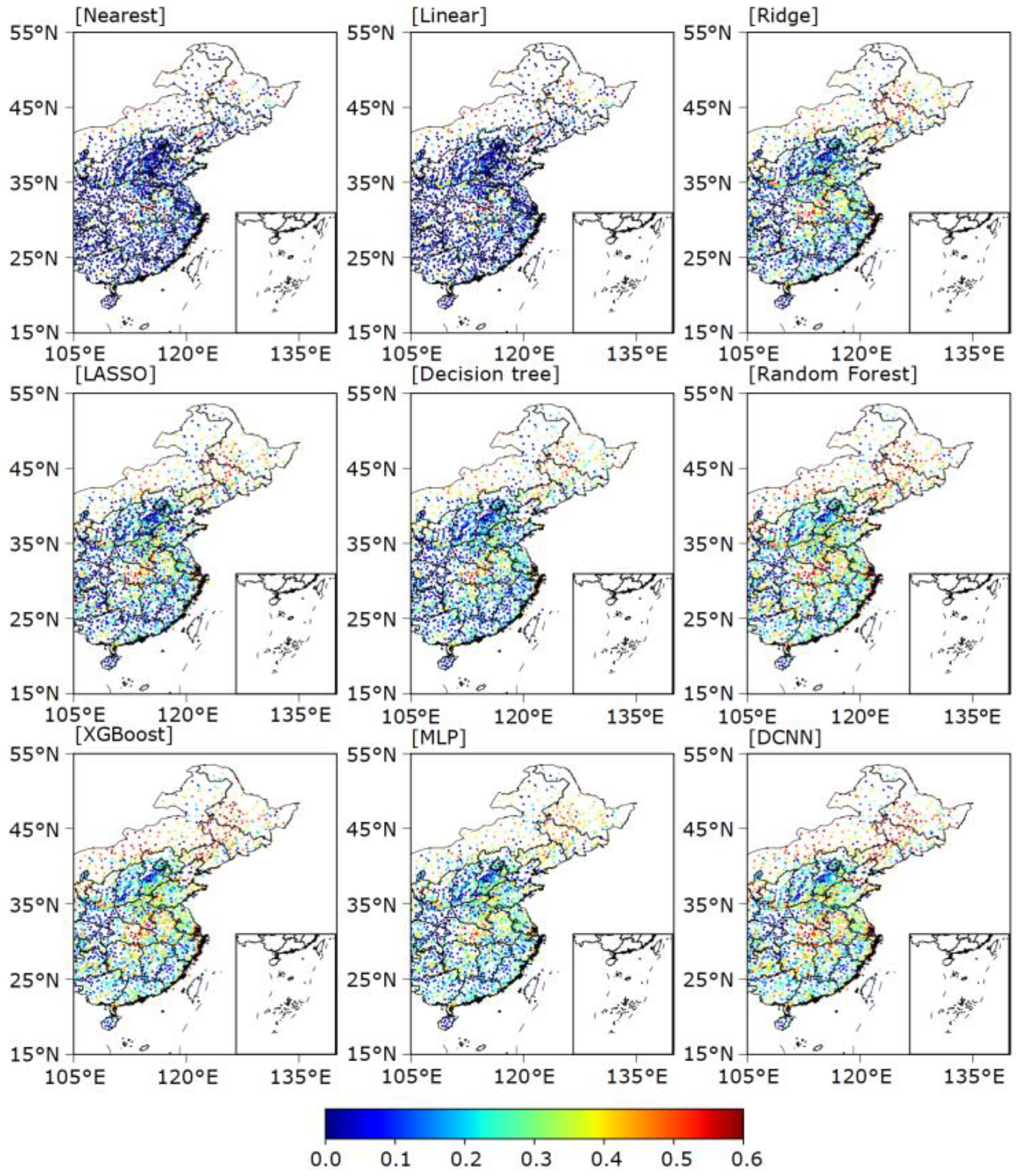
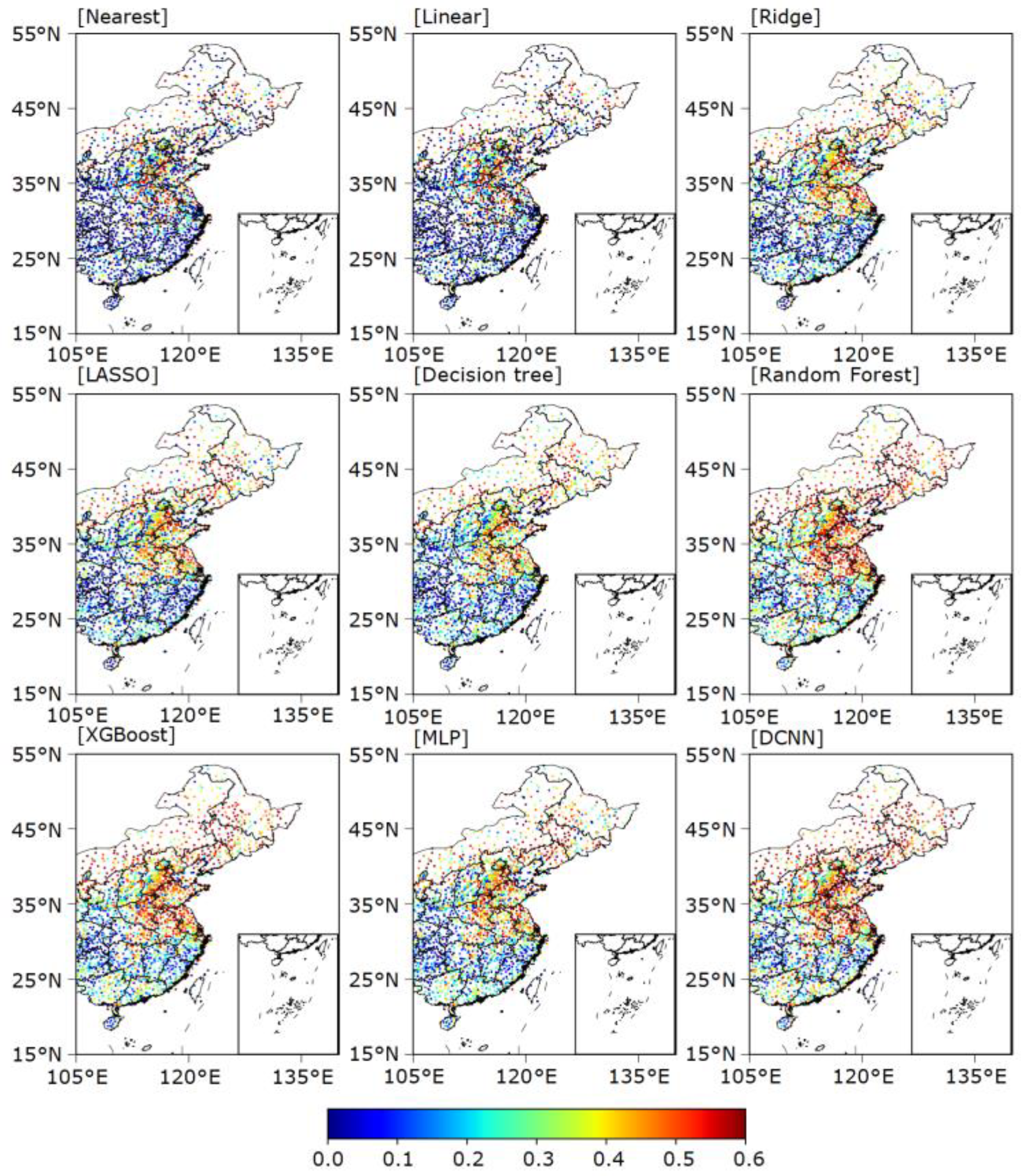
3.2. Spatial Distribution of Estimation Errors

To further assess the performance of the models in different regions, we show the spatial distributions of the RMSEs of wind speeds estimated for summer (Figure 4) and winter (Figure 5) across eastern China. To quantify the effectiveness of estimation by these models in different regions, eastern China is divided into three regions using the 123° E line of longitude and the 32° N line of latitude (Figure 4): the three regions containing land are labeled South, Northeast (NE), and Northwest (NW). For the summer data, the two LMs perform poorly overall, with similar error distributions. The regions with large errors are mainly concentrated in coastal areas, Inner Mongolia, and the Yunnan–Guizhou plateau. The RMSEs for the Yunnan–Guizhou plateau and Inner Mongolia are greater than 1.6 m s−1. The RMSE for the NE (1.2–1.6 m s−1) is better than that for Inner Mongolia and the Yunnan–Guizhou Plateau, but worse than that for Central China. The large errors for these regions indicate strong nonlinearities in the subgrid distribution of WS10. This makes it difficult to resolve such errors by simple linear interpolation. Compared with simple interpolation, both RMs significantly reduce the RMSEs for site-specific WS10 estimation. Compared with the poor performances of the LMs for Inner Mongolia, the Yunnan–Guizhou Plateau, and the NE, the RMSEs of the RMs are reduced by approximately 0.5, 0.2, and 0.2 m s−1, respectively. In plains areas such as the NW, the RMSEs of the RMs are 0.6–1.0 m s−1, significantly better than those of the LMs. The TM and the DL models yield better estimation results than the RMs, with RF, XGBoost, and the DCNN performing significantly better in almost all areas of eastern China. The spatial distributions of RMSE for winter are similar to those for summer, but with slightly larger values. For winter, the DCNN always has the smallest RMSEs among all the models for all three sub-regions (Table 3).
Figure 6 and Figure 7 show the spatial distribution of R2 values between the observed and estimated values for summer and winter. Similar to the distributions of RMSE, the R2 values show that the RMs outperform the LMs but are worse than the ML or DL methods. For the summer data, the RMs show small R2 values (0.15–0.3) for South China coastal provinces. The R2 values for the TMs and DL models are above 0.2 for most sites; RF and the DCNN show yet greater values, above 0.35. For the winter data, RF, XGBoost, and DCNN have R2 values above 0.45, better than those of the LMs (0.2–0.4) and RMs (0.35–0.5). In addition, the R2 of each model is higher for winter than for summer. This is related to the difference in wind speed between the two seasons.
To evaluate the accuracy of the estimated spatial distribution of WS10, Figure 8 and Figure 9 show scatter plots of observations and estimations for the time-averaged WS10 at each site in summer and winter. For the summer, the RMs and TMs show RMSEs that are about 17% and 18% lower than those of the LMs; that of the DCNN, the best model, is 26% lower. Each ML and DL model shows a significantly larger R2 value than the LMs and RMs: those of the LMs are all below 0.09, and those of the RMs are around 0.5. The R2 values of the RF, XGBoost, and DCNN are 0.85, 0.86, and 0.85, respectively, which indicates that these ML and DL models can appropriately handle the spatial distribution of WS10.
For the winter data, the RMSEs of the RMs are at least 10.3% lower than those of the LMs. The reductions of the RMSEs relative to those of the LMs range from 13% for DT to 23% for the DCNN. The RF, XGBoost, and DCNN show the best performance: their respective R2 values are 0.84, 0.82, and 0.83, similar to those for summer.
Overall, the RF, XGBoost, and DCNN outperform the other models for both winter and summer grid-to-site WS10 conversion in eastern China. The DCNN performs best in most areas.

4. Dependence of Estimation Error on Altitude, LUC, and Mean WS10

The ground condition significantly influences the WS10. Previous studies have shown that errors in WS10 estimation for China are strongly correlated with altitude, land use conditions, and WS10 climate values [58]. Therefore, we analyze the dependence of estimation errors on different altitudes, LUC, and temporal mean WS10 when using different grid-to-site WS10 conversion models. The analyses illustrate the extent to which these various models can reflect the influence of these factors and thus assess the applicability of the models to different ground conditions.

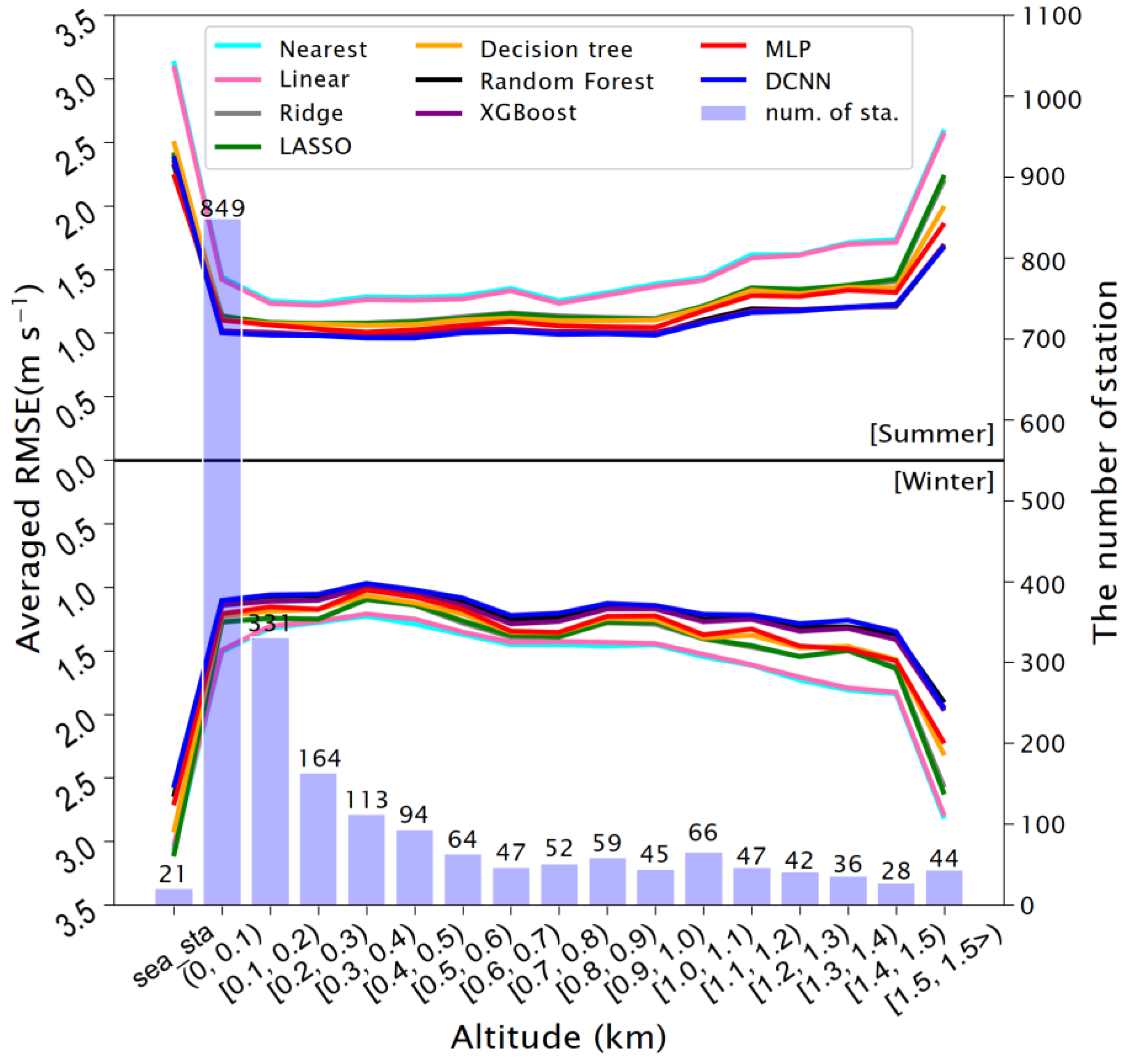
4.1. Dependence of Estimation Error on Altitude

All the sites are grouped into 17 bins at 100 m intervals by elevation. The highest bin represents sites higher than 1500 m. Those with zero elevation are listed separately to show results for sites on the coast and on islands.
Figure 10 shows the averaged RMSEs for WS10 in summer and winter for the altitude bins. The error in estimating WS10 at zero elevation is the largest for both winter and summer. This may be related to the large errors in WS10 values at sea level in the ERA5 datasets [59,60]. For summer, all models have the smallest RMSEs for sites at 200–300 m. For the sites with altitudes over 200 m, the RMSEs essentially increase with increasing height. For the RMs, TMs, and DL models, the RMSEs do not vary significantly for the 0–500 m bins, as they all introduce the altitude as an estimation factor, but their RMSEs increase with altitude for sites above 500 m. In contrast, the DCNN performs best for all altitude bins and does not show significantly varying error with altitude. The results for winter are similar to those in summer.

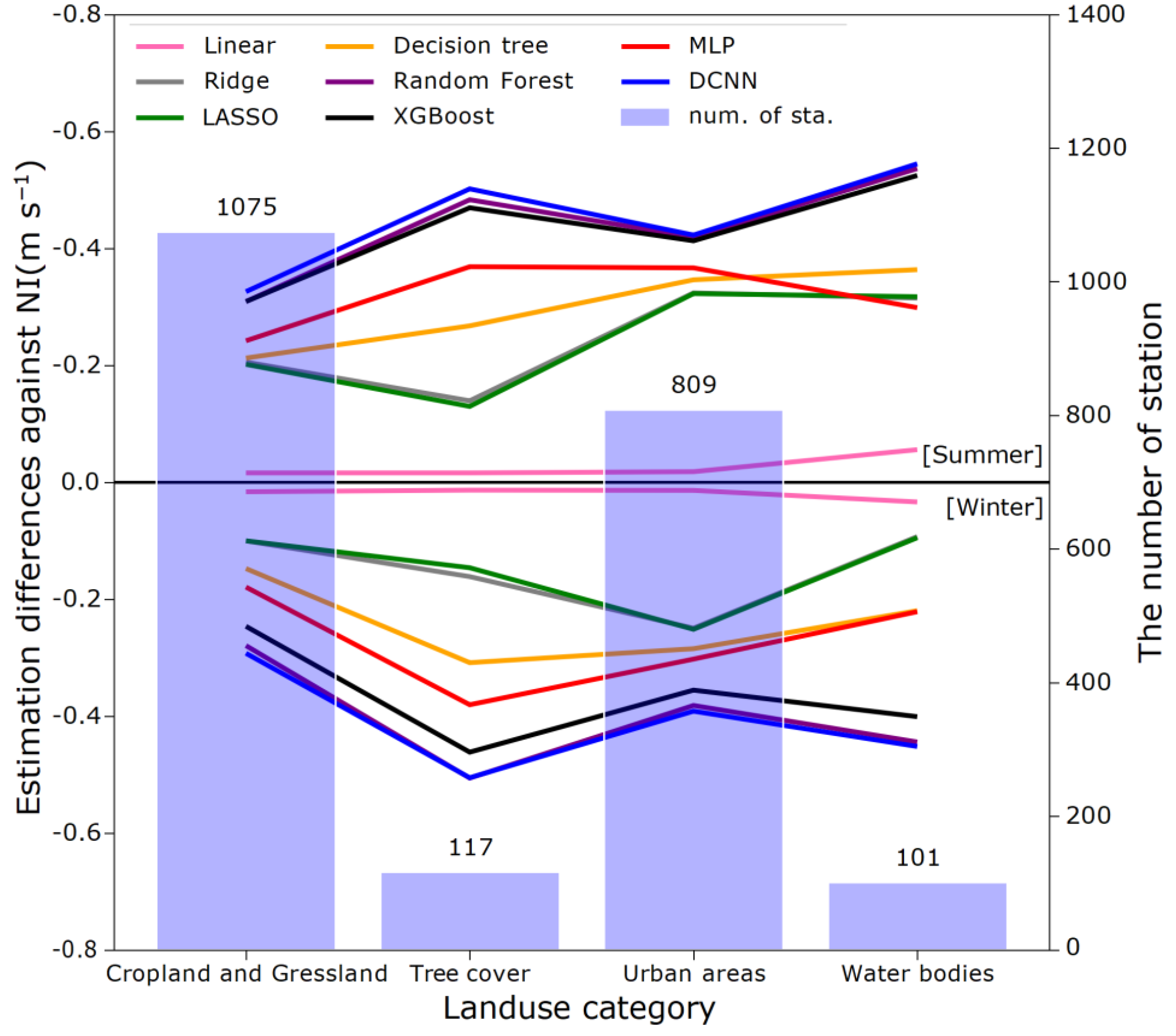
4.2. Dependence of Estimation Error on LUC

We classify all the LUCs into four types according to their typical roughness heights, i.e., low-height surface (including cropland and grassland), tall vegetation (including forests), urban, and water bodies. Figure 11 shows the reductions of RMSE (relative to that of NI) for the various models applied to the winter and summer data considering the four types of LUC. The BI performs similarly to NI for both seasons. For summer, the estimations for low-height surfaces, water bodies, and urban areas are similar for all models: the RMSEs of the RM and MLP are reduced by 0.2–0.3 m s−1 in comparison with that of NI. The RMSEs of RF, XGBoost, and DCNN are decreased by 0.3–0.5 m s−1, mainly due to the improved estimation of WS10 over tall vegetation. The results for winter are similar to those for summer. Overall, the DCNN gives the best estimations over all four LUC types. RF performs slightly worse than the DCNN, but much better than the other models.

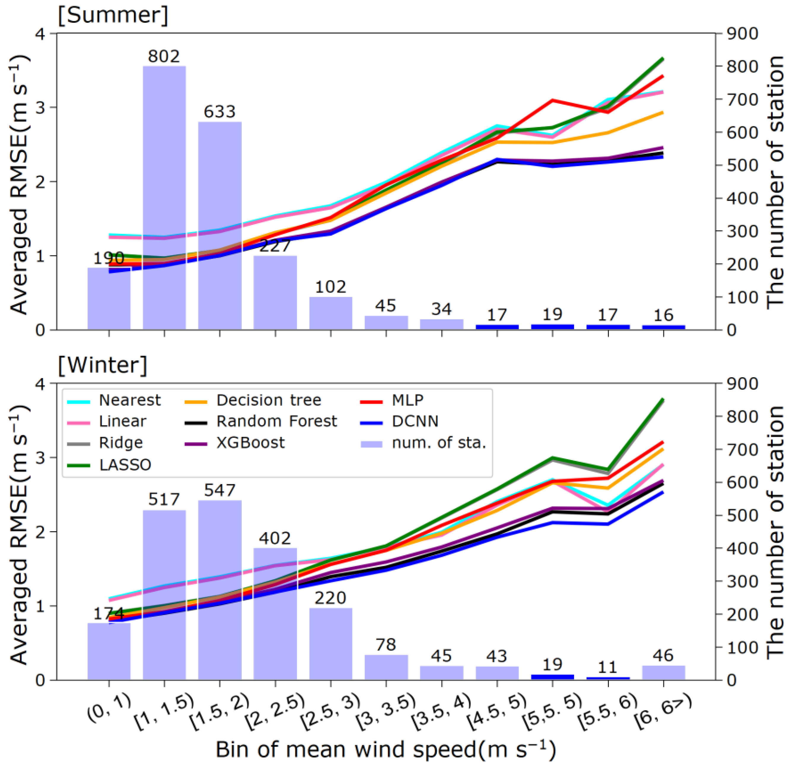
4.3. Dependence of Estimation Error on Mean WS10

Figure 12 shows the distribution of the estimated RMSE with respect to the mean wind speed. In areas where the mean WS10 is between 0 and 2.5 m s−1, the RMs, TMs, ML, and DL models perform similarly, much better than the LMs. In regions with mean WS10 greater than 2.5 m s−1, the RMSEs of both RMs and the MLP are close to those of the LMs, indicating that these models lose applicability to these areas. However, DCNN, XGBoost, and RF maintain their good estimation performance. The results for winter are similar to those for summer in areas with WS10 ≤ 2.5 m s−1. However, for areas with WS10 > 2.5 m s−1, the RMs, MLP, and DT provide poor estimations, even worse than the two LMs. While XGBoost and RF perform better than those models, they are close to the two LMs in areas with 5.5–6.0 m s−1 mean WS10. Finally, the DCNN performs well in winter, with a significant advantage over the other eight models.

5. Conclusions

Interpolation is an important tool to fill gaps in gridded data to estimate WS10 at a given sites for wind speeds. Traditional interpolation based on linear methods does not reflect the strong nonlinearity of the grid-to-site conversion of WS10. Currently, models employing ML and DL are emerging as effective ways to deal with nonlinear interpolation problems. However, the effectiveness and applicability of various ML and DL methods become issues when applying a unified model to a large area like China. Therefore, we discuss the applicability of multiple ML and DL methods to estimate WS10 in winter and summer at sites across eastern China, and we compare these models with traditional LMs and RMs. The following conclusions are obtained:
(1)
Overall, the estimation error of WS10 is smaller for summer than for winter for all nine grid-to-site WS10 models;
(2)
The DT-based, ML, and DL models that use multiple input variables outperform the traditional LMs that use only gridded WS10;
(3)
Among these more elaborate models, the RF, XGBoost, and DCNN perform best;
(4)
The DCNN is the overall best model as it performs robustly for sites at different altitudes and with the varying LUCs and local mean WS10, indicating that it can reflect the nonlinear relationships among these variables and WS10.
The main shortcoming of the ML and DL models for grid-to-site WS10 conversion is that their performance varies significantly across regions, which limits their applicability as unified models. For example, none of these models provide satisfactory WS10 estimations for northern Inner Mongolia, possibly owing to the lack of physical constraints of the surface layer in these unified data-based models. Similarly, surface wind speed interpolation in western China is not discussed in this paper because all the methods described above would lose validity in this region due to its complex climate, topography, and land condition. A current proposal by Feng et al. [61] aims to develop a physics–data hybrid model that improves WS10 estimation for almost all sites in China. However, the model does not apply any ML or DL structures, which would be detrimental to its handling of complex meteorology and ground conditions. Hence, the full integration of a physical model and ML or DL requires further study. In addition, this paper mainly calculates the site-specific WS10 based on ERA5 reanalysis datasets. When these ML models are used for the grid-to-site conversion from data of numerical weather prediction, it is necessary to make an ML model with more input variables and a more complex structure to handle both the interpolation error and the error between forecasts and reanalyses.

Supplementary Materials

The following supporting information can be downloaded at: https://www.mdpi.com/article/10.3390/atmos14010142/s1, Figure S1: Scatterplot for all seven non-linear models on the summer training sets; Figure S2: Scatterplot for all seven non-linear models on the summer validation sets; Figure S3: Same as Figure S1 but for winter training sets; Figure S4: Same as Figure S2 but for winter validation sets; Table S1: Landuse value and label.

Author Contributions

J.Z.: Data Processing, Code Implementation, Literature Research, Result Visualization and Result Analysis, Writing—Original Draft. J.F.: Supervised, Conceptualization, Providing Resources, Writing—Original Draft, Writing—Review, and Editing. X.Z.: Supervised, Writing—Review, and Editing. Y.L.: Writing—Review. F.Z.: Provides design ideas for the DCNN model. All authors have read and agreed to the published version of the manuscript.

Funding

This research is supported by the National Key R&D Program of China (2021YFC3000901) and the National Natural Science Foundation of China (42275009, 41905037; 42275059).

Institutional Review Board Statement

Not applicable.

Informed Consent Statement

Not applicable.

Data Availability Statement

Data and code are available upon request from the corresponding author (Jin Feng).

Conflicts of Interest

The authors declare no competing interest.

References

  1. Hoolohan, V.; Tomlin, A.S.; Cockerill, T. Improved near surface wind speed predictions using Gaussian process regression combined with numerical weather predictions and observed meteorological data. J. Renew. Energy 2018, 126, 1043–1054. [Google Scholar] [CrossRef]
  2. Bernier, N.B.; Bélair, S.; Bilodeau, B.; Tong, L. Assimilation and High-Resolution Forecasts of Surface and Near Surface Conditions for the 2010 Vancouver Winter Olympic and Paralympic Games. J. Pure Appl. Geophys. 2014, 171, 243–256. [Google Scholar] [CrossRef] [Green Version]
  3. Prasanna, V.; Choi, H.W.; Jung, J.; Lee, Y.G.; Kim, B.J. High-Resolution Wind Simulation over Incheon International Airport with the Unified Model’s Rose Nesting Suite from KMA Operational Forecasts. J. Asia-Pacific J. Atmos. Sci. 2018, 54, 187–203. [Google Scholar] [CrossRef]
  4. Zhang, H.P.; Zhou, X.; Dai, W. A Preliminary on Applicability Analysis of Spatial Interpolation Method. J. Geogr. Geo-Inf. Sci. 2017, 33, 14–18+105. [Google Scholar] [CrossRef]
  5. Jin, L. A Review of Spatial Interpolation Methods for Environmental Scientists. J. Rec. Geosci. Aust. 2008, 137–145. Available online: https://www.researchgate.net/profile/Jin-Li-74/publication/246546630_A_Review_of_Spatial_Interpolation_Methods_for_Environmental_Scientists/links/56f9ccb408ae95e8b6d40461/A-Review-of-Spatial-Interpolation-Methods-for-Environmental-Scientists.pdf (accessed on 4 January 2023).
  6. Han, E.; Wen, X.; Wang, B.; Yang, F.; Shen, H.; Zhu, M. The Application of Meteorological Reanalysis Data for Wind Tower Data Interpolation at Complex Mountain Area Wind Farm. J. Jiangxi Sci. 2017, 2, 21–26. Available online: https://kns.cnki.net/kcms/detail/detail.aspx?dbcode=CJFD&dbname=CJFDLAST2017&filename=JSKX201702004&uniplatform=NZKPT&v=2poMa-B8Wa2X96cEEBiIHHHYzhB9QNoty3WRbEIwij288WUWMjGby1jrDD4v1mK_, (accessed on 4 January 2023).
  7. Du, J.; Peng, L.; Liu, Y.; Pan, L.; Wang, L.; Cao, Y. Combined interpolation model for wind speed measurement missing of wind farm. J. Electr. Power Autom. Equipment 2015, 9, 129–133. Available online: https://en.cnki.com.cn/Article_en/CJFDTOTAL-DLZS201509020.htm (accessed on 4 January 2023).
  8. Ambach, D.; Croonenbroeck, C. Using the lasso method for space-time short-term wind speed predictions. J. Eprint arXiv 2015. Available online: https://www.esearchgate.net/publication/271447832_Using_the_lasso_method_for_space-time_short-term_wind_speed_predictions (accessed on 4 January 2023).
  9. Alalami, M.A.; Maalouf, M.; El-Fouly, T. Wind Speed Forecasting Using Kernel Ridge Regression with Different Time Horizons. In Theory and Applications of Time Series Analysis, Selected Contributions from ITISE; Springer: Berlin/Heidelberg, Germany, 2019; pp. 191–203. [Google Scholar] [CrossRef]
  10. Davy, R.J.; Woods, M.J.; Russell, C.; Coppin, P.A. Statistical Downscaling of Wind Variability from Meteorological Fields. J. Bound. Layer Meteorol. 2010, 135, 161–175. [Google Scholar] [CrossRef]
  11. Salameh, T.; Drobinski, P.; Vrac, M.; Naveau, P. Statistical downscaling of near-surface wind over complex terrain in southern France. J. Meteorol Atmos. Phys. 2009, 10, 253–265. [Google Scholar] [CrossRef]
  12. Wilcox, B.; Yip, M.C. SOLAR-GP: Sparse, Online, Locally Adaptive Regression using Gaussian Processes for Bayesian Robot Model Learning and Control. J. IEEE Robot. Autom. Lett. 2020, 5, 2832–2839. Available online: https://www.docin.com/p-2370665226.html (accessed on 4 January 2023). [CrossRef]
  13. Wang, N.; Pan, M.X.; Huang, J.Q. Nonlinear Model Predictive Control for Turbo-Shaft Engine Based on the Online Sliding Sequence Kernel Extreme Learning Machine. J. Aeroengine. 2018, 5, 48–54. Available online: http://en.cnki.com.cn/Article_en/CJFDTotal-HKFJ201805007.htm (accessed on 4 January 2023).
  14. Kaur, H.; Pham, N.; Fomel, S. Seismic data interpolation using deep learning with generative adversarial networks. J. Geophys.l Prospecting 2021, 69, 2. [Google Scholar] [CrossRef]
  15. Leirvik, T.; Yuan, M. A Machine Learning Technique for Spatial Interpolation of Solar Radiation Observations. J. Earth Space Sci. 2021, 8, 527. [Google Scholar] [CrossRef]
  16. Manucharyan, G.E.; Siegelman, L.; Klein, P. A Deep Learning Approach to Spatiotemporal Sea Surface Height Interpolation and Estimation of Deep Currents in Geostrophic Ocean Turbulence. J. Adv. Modeling Earth Syst. 2021, 13, 965. [Google Scholar] [CrossRef]
  17. Yatheendradas, S.; Kumar, S. A Novel Machine Learning–Based Gap-Filling of Fine-Resolution Remotely Sensed Snow Cover Fraction Data by Combining Downscaling and Regression. J. Hydrometeorol. 2022, 23, 637–658. Available online: https://journals.ametsoc.org/view/journals/hydr/23/5/JHM-D-20-0111.1.xml (accessed on 4 January 2023).
  18. Alizamir, M.; Moghadam, M.A.; Monfared, A.H.; Shamsipour, A. Statistical downscaling of global climate model outputs to monthly precipitation via extreme learning machine: A case study. J. Environ. Prog. Sustain. Energy 2018, 37, 1853–1862. [Google Scholar] [CrossRef]
  19. Dalto, M.; Matusko, J.; Vasak, M. Deep neural networks for ultra-short-term wind forecasting. In Proceedings of the IEEE International Conference on Industrial Technology, Seville, Spain, 17–19 March 2015. [Google Scholar] [CrossRef]
  20. Zhang, C.Y.; Chen, C.; Gan, M.; Chen, L. Predictive deep Boltzmann machine for multiperiod wind speed forecasting. J. IEEE Transac. Sustain. Energy 2015, 6, 1416–1425. [Google Scholar] [CrossRef]
  21. Wang, J.; Yang, Z. Ultra-short-term wind speed forecasting using an optimized artificial intelligence algorithm. J. Renew. Energy 2021, 171, 5. [Google Scholar] [CrossRef]
  22. Niu, D.; Sun, L.; Yu, M.; Wang, K. Point and Interval Forecasting of Ultra-Short-Term Wind Power Based on Data-Driven Method and Hybrid Deep Learning Model. J. Soc. Sci. Electron. Publishing 2022, 254, 124384. [Google Scholar] [CrossRef]
  23. Giorgi, M.; Russo, M.G.; Ficarella, A. Short-term wind forecasting using artificial neural networks (ANNs). J. WIT Transac. Ecol. Environ. 2009, 121, 12. Available online: https://www.witpress.com/elibrary/wit-transactions-on-ecology-and-the-environment/121/20242 (accessed on 4 January 2023).
  24. Qiaomu, Z.; Jinfu, C.; Lin, Z.; Duan, X.; Liu, Y. Wind Speed Prediction with Spatio–Temporal Correlation: A Deep Learning Approach. J. Energ. 2018, 11, 705. Available online: https://ideas.repec.org/a/gam/jeners/v11y2018i4p705-d137311.html (accessed on 4 January 2023).
  25. Li, H.; Wang, J.; Lu, H.; Guo, Z. Research and application of a combined model based on variable weight for short term wind speed forecasting. J. Renew. Energy 2018, 116, 669–684. [Google Scholar] [CrossRef]
  26. Zhou, C.; Haochen, L.I.; Chen, Y.U. A station-data-based model residual machine learning method for fine-grained meteorological grid prediction. J. Appl. Math. Mechanics 2022, 43, 12. [Google Scholar] [CrossRef]
  27. Saeed, A.; Li, C.; Gan, Z.; Xie, Y.; Liu, F. A simple approach for short-term wind speed interval prediction based on independently recurrent neural networks and error probability distribution. J. Energy 2022, 238, 122012. [Google Scholar] [CrossRef]
  28. Salcedo-Sanz, S.; Pérez-Bellido, M.; Ortiz-García, E.G.; Portilla-Figueras, A.; Prieto, L.; Paredes, D. Hybridizing the fifth-generation mesoscale model with artificial neural networks for short-term wind speed prediction. J. Renew. Energy 2009, 34, 1451–1457. [Google Scholar] [CrossRef]
  29. Nian, L.; Zhongwei, Y.; Xuan, T.; Jiang, J.; Haochen, L.; Jiangjiang, X.; Xiao, L.; Rui, R.; Yi, F. Meshless Surface Wind Speed Field Reconstruction based on Machine Learning. J. Adv. Atmos. Phys. 2022, 39, 1721–1733. [Google Scholar] [CrossRef]
  30. Oh, M.; Lee, J.; Kim, J.; Kim, H. Machine learning-based statistical downscaling of wind resource maps using multi-resolution topographical data. Wind. Energy 2022, 25, 1121–1141. [Google Scholar] [CrossRef]
  31. Veronesi, F.; Grassi, S.; Raubal, M. Statistical learning approach for wind resource assessment. J. Renew. Sustain. Energy Rev. 2016, 56, 836–850. [Google Scholar] [CrossRef]
  32. Koo, J.; Han, G.D.; Choi, H.J.; Shim, J.H. Wind-speed prediction and analysis based on geological and distance variables using an artificial neural network: A case study in South Korea. J. Energy 2015, 93, 1296–1302. [Google Scholar] [CrossRef]
  33. Barati, H.; Haroonabadi, H.; Zadehali, R. Wind speed forecasting in South Coasts of Iran: An Application of Artificial Neural Networks (ANNs) for Electricity Generation using Renewable Energy. J. Bull. Environ. Pharmacol. Life Sci. 2013, 2, 37–39. Available online: https://bepls.com/may_2013/4.pdf (accessed on 4 January 2023).
  34. Wu, Y.; Huang, S.X.; Chen, Y.J.Z. Application of machine learning in forecasting maximum wind speed of typhoon in Guangxi. J. Meteorol. Res. Appl. 2021, 42, 26–31. [Google Scholar] [CrossRef]
  35. Zhang, Z.; Ye, L.; Qin, H.; Liu, Y.; Wang, C.; Yu, X.; Yin, X.; Li, J. Wind speed prediction method using Shared Weight Long Short-Term Memory Network and Gaussian Process Regression. J. Appl. Energy 2019, 247, 270–284. Available online: https://ideas.repec.org/a/eee/appene/v247y2019icp270-284.html (accessed on 4 January 2023). [CrossRef]
  36. Wu, J.; Zha, J.; Zhao, D. Evaluating the effects of land use and cover change on the decrease of surface wind speed over China in recent 30 years using a statistical downscaling method. J. Clim. Dyn. 2017, 48, 131–149. [Google Scholar] [CrossRef] [Green Version]
  37. Zhao, C.; Zhang, T.; Wang, W.; Liu, Y.; Zeng, D.; Li, Y. Impacts of Land-use Data on the Simulation of 10 m Wind Speed in Northwest China. J. Arid Meteorol. 2018, 3, 60–67. Available online: http://en.cnki.com.cn/Article_en/CJFDTOTAL-GSQX201803007.htm (accessed on 4 January 2023).
  38. Li, Y.; Chen, Y.; Li, Z. Effects of land use and cover change on surface wind speed in China. J. Arid Land 2019, 11, 345–356. Available online: https://d.wanfangdata.com.cn/periodical/ghqkx201903003 (accessed on 4 January 2023). [CrossRef] [Green Version]
  39. Ngo, T.; Letchford, C. A comparison of topographic effects on gust wind speed. J. Wind Eng. Ind. Aerodyn. 2008, 96, 2273–2293. [Google Scholar] [CrossRef]
  40. Zurański, J.A. Orographic effects on strong winds in Poland. J. Wind Eng. Ind. Aerodyn. 1992, 41, 417–426. [Google Scholar] [CrossRef]
  41. Zhang, Z.B.; Yang, Y.; Zhang, X.P.; Chen, Z. Wind speed changes and its influencing factors in Southwestern China. J. Acta Ecol. Sin. 2014, 34, 471–481. [Google Scholar] [CrossRef]
  42. Fu, C.; Yu, J.; Zhang, Y.; Hu, S.; Ouyang, R.; Liu, W. Temporal variation of wind speed in China for 1961–2007. J. Theor. Appl. Climatol. 2011, 104, 313–324. [Google Scholar] [CrossRef]
  43. Bilbao, I.; Bilbao, J.; Feniser, C. Adopting Some Good Practices to Avoid Overfitting in the Use of Machine Learning. J. World Sci. Eng. Acad. Soc. 2018, 17, 274–279. Available online: https://www.nstl.gov.cn/paper_detail.html?id=e2d7403ba73d508a6f86a2decba5b64d (accessed on 4 January 2023).
  44. Hoerl, A.; Kennard, R. Ridge Regression: Biased Estimation for Nonorthogonal Problems. J. Technometrics 1970, 12, 5–67. [Google Scholar] [CrossRef]
  45. Hans, C. Bayesian lasso regression. J. Biometrika 2009, 96, 835–845. Available online: https://ideas.repec.org/a/oup/biomet/v96y2009i4p835-845.html (accessed on 4 January 2023). [CrossRef]
  46. Breiman, L.I.; Friedman, J.H.; Olshen, R.A.; Stone, C.J. Classification and Regression Trees. Wadsworth. J. Biom. 1984, 40, 358. Available online: https://www.docin.com/p-1798845890.html (accessed on 4 January 2023).
  47. Svetnik, V.; Liaw, A.; Tong, C.; Culberson, J.C.; Sheridan, R.P.; Feuston, B.P. Random Forest: A classification and regression tool for compound classification and QSAR modeling. J. Chem. Inf. Comput. Sci. 2003, 43, 1947–1958. [Google Scholar] [CrossRef]
  48. Chen, T.; Guestrin, C. XGBoost: A Scalable Tree Boosting System. In Proceedings of the 22nd ACM SIGKDD International Conference on Knowledge Discovery and Data Mining, San Francisco, CA, USA, 13–17 August 2016. [Google Scholar] [CrossRef] [Green Version]
  49. Bauer, E.; Kohavi, R. An Empirical Comparison of Voting Classification Algorithms: Bagging, Boosting, and Variants. J. Mach. Learn. 1999, 36, 105–139. Available online: https://link.springer.com/article/10.1023/A:1007515423169 (accessed on 4 January 2023). [CrossRef]
  50. Wang, A.; Xu, L.; Li, Y.; Xing, J.; Chen, X.; Liu, K.; Liang, Y.; Zhou, Z. Random-forest based adjusting method for wind forecast of WRF model. J. Comput. Geosci. 2021, 1–2, 104842. [Google Scholar] [CrossRef]
  51. Pooja, V.R.; Farzana, B.S.; Saranya, M.; Vanathi, B. Wind speed prediction using tree ensemble. J. IJARIIT 2018, 4, 2454-132X. Available online: https://www.ijariit.com/manuscripts/v4i2/V4I2-1843.pdf (accessed on 4 January 2023).
  52. Kim, T.; Adali, T. Fully Complex Multi-Layer Perceptron Network for Nonlinear Signal Processing. J. Signal Process. Syst. 2002, 32, 29–43. Available online: https://link.springer.com/article/10.1023/A%3A1016359216961 (accessed on 4 January 2023).
  53. Srivastava, N.; Hinton, G.; Krizhevsky, A.; Sutskever, I.; Salakhutdinov, R. Dropout: A simple way to prevent neural networks from overfitting. J. Mach. Learn. Res. 2014, 15, 1929–1958. Available online: https://www.jmlr.org/papers/v15/srivastava14a.html (accessed on 4 January 2023).
  54. Zhu, F.; Li, X.; Qin, J.; Yang, K.; Cuo, L.; Tang, W.; Shen, C. Integration of Multisource Data to Estimate Downward Longwave Radiation Based on Deep Neural Networks. IEEE Trans. Geosci. Remote. Sens. 2021, 60, 4103015. [Google Scholar] [CrossRef]
  55. Yang, X. An Overview of the Attention Mechanisms in Computer Vision. J. Phys. Conf. Ser. 2020, 1693, 012173. Available online: https://iopscience.iop.org/article/10.1088/1742-6596/1693/1/012173 (accessed on 4 January 2023). [CrossRef]
  56. Huang, G.; Liu, Z.; Van Der Maaten, L.; Weinberger, K.Q. Densely connected convolutional networks. In Proceedings of the IEEE Conference on Computer Vision and Pattern Recognition, Honolulu, HI, USA, 21–26 July 2017; pp. 4700–4708. Available online: https://arxiv.org/pdf/1608.06993.pdf (accessed on 4 January 2023).
  57. Woo, S.; Park, J.; Lee, J.Y.; Kweon, I.S. Cbam: Convolutional Block Attention Module. In Proceedings of the European Conference on Computer Vision (ECCV); Springer: Cham, Switzerland, 2018; pp. 3–19. [Google Scholar] [CrossRef]
  58. Gong, X.; Zhu, R.; Chen, L. Characteristics of Near Surface Winds over Different Underlying Surfaces in China: Implications for Wind Power Development. J. Meteorol. Res. 2019, 33, 349–362. Available online: http://qikan.cqvip.com/Qikan/Article/Detail?id=7001971633 (accessed on 4 January 2023). [CrossRef]
  59. Meng, X.; Guo, J.; Han, Y.; Yongqing, H. Preliminarily assessment of ERA5 reanalysis data. J. Mar. Meteorol. 2018, 1, 94–102. [Google Scholar] [CrossRef]
  60. Wang, G.; Wang, X.; Wang, H.; Hou, M.; Li, Y.; Fan, W.; Liu, Y. Evaluation on monthly sea surface wind speed of four reanalysis data sets over the China seas after 1988. Acta Oceanol. Sin. 2020, 39, 83–90. [Google Scholar] [CrossRef]
  61. Feng, J.; Huang, X.; Li, Y. Improving Surface Wind Speed Forecasts Using an Offline Surface Multilayer Model with Optimal Ground Forcing. J. Adv. Model. Earth Syst. 2022, 14, 10. [Google Scholar] [CrossRef]
Figure 1. Scatter plots of wind speeds estimated by all nine grid-to-site conversion models and observed values for the summer test dataset. The value of colorbar is represented log 2 k e r n e l   d e n s i t y × 100 , 000 .
Atmosphere 14 00142 g001
Figure 2. As Figure 1 but for the winter test dataset.
Atmosphere 14 00142 g002
Figure 3. Probability density distribution of RMSEs of interpolation results for eastern China from different methods (μ: RMSE value corresponding to the peak, var: variance of all RMSEs).
Atmosphere 14 00142 g003
Figure 4. Spatial distribution of RMSEs of summer wind speeds across eastern China estimated by different interpolation methods.
Atmosphere 14 00142 g004
Figure 5. Spatial distribution of RMSEs of winter wind speeds across eastern China estimated by different interpolation methods.
Atmosphere 14 00142 g005
Figure 6. Spatial distribution of R2 values for summer wind speeds across eastern China estimated by different interpolation methods.
Atmosphere 14 00142 g006
Figure 7. Spatial distribution of R2 values for winter wind speeds across eastern China estimated by different interpolation methods.
Atmosphere 14 00142 g007
Figure 8. Correlation analysis of observed summer wind speeds and those predicted by each method.
Atmosphere 14 00142 g008
Figure 9. Correlation analysis of observed winter wind speeds and those predicted by each method.
Atmosphere 14 00142 g009
Figure 10. Comparison of errors in estimated wind speed at sites at different altitudes. Bars indicate the number of sites at each altitude interval, and lines give the average RMSE of winter and summer wind speeds estimated using each method at the corresponding altitude.
Atmosphere 14 00142 g010
Figure 11. Comparison of errors in estimation of wind speed at sites with different land use types. Bars show the number of sites with each land use type, and lines compare the errors in winter and summer wind speeds estimated using each method at the corresponding altitude with the error of the estimation by linear interpolation. Note: the vertical Comparison method axis represents the difference in the error of the given method and that of NI (i.e., RMSE of the given method—the RMSE of linear NI). The land use types represent different underlying surface conditions, classified as arable and grassland (low vegetation), forest (high vegetation), urban areas, and water bodies.
Atmosphere 14 00142 g011
Figure 12. Comparison of errors in estimation of wind speed at sites with different average WS10. Bars show the number of sites with WS10 within each interval, and lines show the average RMSE of winter and summer wind speeds estimated using each method for the corresponding interval.
Atmosphere 14 00142 g012
Table 1. Summary of models used in this study.
TypeLinear
Interpolation
Regression
Models
Tree
Models
Deep Learning
Models
NameNearest
Bilinear
Ridge
Lasso
Decision Tree
Random Forest
XGboost
MLP
DCNN
Table 2. Summary of data used in this study (“m” represents millions).
DatasetTrainingValidationTesting
SummerWinterSummerWinterSummerWinter
Year20192020201920202020202120202021
Month6, 7, 86121, 2, 127182
Num. of times976976248248248224
Num. of samples2.05 m2.05 m0.52 m0.52 m0.52 m0.47 m
Table 3. RMSEs and number of sites in three sub-regions of eastern China in summer and winter.
AreaSouth ChinaNortheast ChinaNorth China
SummerWinterSummerWinterSummerWinter
Nearest1.451.361.351.551.401.59
Linear1.431.341.341.551.381.57
Ridge1.201.201.101.401.141.43
Lasso1.221.201.101.401.151.42
Decision Tree1.161.121.101.331.141.40
Random Forest1.061.021.001.201.051.26
XGboost1.081.060.991.241.041.29
MLP1.141.101.051.341.111.37
DCNN1.041.020.991.181.031.24
Num. of sites9111018173
Disclaimer/Publisher’s Note: The statements, opinions and data contained in all publications are solely those of the individual author(s) and contributor(s) and not of MDPI and/or the editor(s). MDPI and/or the editor(s) disclaim responsibility for any injury to people or property resulting from any ideas, methods, instructions or products referred to in the content.

