Simulation of the Spatiotemporal Distribution of PM_2.5 Concentration Based on GTWR-XGBoost Two-Stage Model: A Case Study of Chengdu Chongqing Economic Circle

Abstract

Natural environmental factors and human activity intensity factors, the two main factors that affect the spatial and temporal distribution of PM_2.5 concentration near the surface, have different mechanisms of action on PM_2.5 concentration. In this paper, a GTWR-XGBoost two-stage sequential hybrid model is proposed aiming at detecting the expression of spatiotemporal heterogeneity in the traditional machine learning retrieval model of PM_2.5 concentration and the difficulty of expressing the complex nonlinear relationship in the statistical regression model. In the first stage, the natural environmental factors are used to predict PM_2.5 concentration with spatiotemporal characteristics by collinearity diagnosis method and Geographically and Temporally Weighted Regression method (GTWR). In the second stage, the simulation results in the first stage and the natural factors eliminated through LUR stepwise regression in the first stage are into the XGBoost model together with the human activity intensity factors in the buffer zone with the best correlation coefficient of PM_2.5, and finally the temporal and spatial distribution of PM_2.5 concentration. Taking the Chengdu Chongqing Economic Circle as an example, the proposed model is used to retrieve PM_2.5 concentration and compared with the single GTWR, XGBoost, and coupling model published recently. The experimental results show that the R², RMSE, and MAE of the GTWR-XGBoost two-stage model cross-validation are 0.92, 5.44 ug·m⁻³, and 4.12 ug·m⁻³, respectively. Compared with the above single models, R² increased by 0.01 and 0.12, and MAE decreased by more than 0.11 and 3.1, respectively. Compared with the coupling model published recently, R² is increased by 0.02, and MAE is reduced by more than 0.4. In addition, the PM_2.5 concentration in Chengdu Chongqing showed obvious seasonal temporal and spatial changes, and the influence ratios of natural environmental factors and human activity intensity activities factors on PM_2.5 were 0.66 and 0.34. The results show that the GTWR-XGBoost two-stage Model can not only describe the heterogeneity and objectively reflect the complex nonlinear relationship between the phenomenon and the influencing factors, but also enhance the interpretability of the phenomenon when simulating the spatiotemporal distribution characteristics of PM_2.5 concentration.

1. Introduction

PM_2.5, the fine particulate matter with aerodynamic particle size ≤ 2.5 μm in the environment [1], has attracted much attention. It not only affects the quality of the atmospheric environment, but also poses a serious threat to human health due to its strong activity and easy adhesion of toxic and harmful substances [2]. Studies have shown that Aerosol Optical Depth (AOD) retrieved by satellite remote sensing is correlated with PM_2.5 [3,4]. This means that using remote sensing data to invert the relationship between AOD and PM_2.5 content values monitored in the same region at the same time can achieve the effect of monitoring PM_2.5 using AOD. Compared with the traditional station monitoring method, the method of obtaining the spatial distribution of PM_2.5 by remote sensing inversion has the advantages of wide coverage, low cost, repeatable observation, fast acquisition speed, and long time series, and can well fill the data gap left by sparse ground monitoring stations [5,6].

Early simple linear regression models [7] and multiple linear regression models [8,9] were used to predict the spatiotemporal distribution of PM_2.5 concentration. However, due to the non-stationarity of local spatiotemporal data of PM_2.5 and AOD, the retrieval accuracy was not high.

Like any other spatial phenomenon, PM_2.5 and AOD are also affected by spatiotemporal heterogeneity. Therefore, the Linear Mixed Effects model (LME) [10,11], Geographically Weighted Regression model (GWR) [12,13], Geographically and Temporally Weighted regression (GTWR) [14], ANN-GWR [15] and other mathematical models have been successively used to retrieve PM_2.5 concentration to better reveal the spatiotemporal heterogeneity of its distribution. The research also shows that these methods can improve the retrieval accuracy of PM_2.5 to different degrees.

With the growth of data volume and prediction variables, methods such as random forest (RF) and deep learning (DL) have also been applied to retrieve PM_2.5 concentration [16,17,18].

The PM_2.5 retrieval model based on machine learning has roughly experienced the evolution from simple linear regression, linear mixed model, geographically weighted regression, decision tree model, deep learning model, and a mixture of multiple models.

In recent years, the combination of different models has been applied to the spatiotemporal prediction of PM_2.5 concentration due to their methodological flexibility and convenience. Compared with many machine learning models, the XGBoost model has better performance in retrieving PM_2.5 concentration [19]. Taking Taiwan as an example, Wong shows that combining the mixed Kriging LUR model with the XGBoost algorithm (LUR-XGBoost) can well estimate PM_2.5 concentration. The Spatiotemporal Random Forest (STRF) model [20] was used to retrieve PM_2.5 concentration, and its performance was proved to be better than that of some statistical regression models. Subsequently, landuse regression combined with random forest (LUR-RF) [21], GAM-RF [22], and other mixed models have a good performance in retrieving PM_2.5 concentration. At the same time, Machine learning combined with deep learning to extract spatiotemporal features for PM_2.5 prediction and inversion may become a new trend due to higher prediction accuracy and stronger generalization ability [23,24,25].

Previous studies have shown that GTWR has the advantage of retrieving the distribution of PM_2.5 by considering the spatiotemporal heterogeneity of natural environment factors. XGBoost has the advantage of combining the driving factors of multiple complex nonlinear relationships without considering the multilinear problem between variables and has a higher performance. However, their independent applications have obvious defects. Inspired by the idea of a sequential hybrid model, how to give play their respective advantages through model integration is a problem that needs further discussion.

Given this, this paper employed the Chengdu Chongqing Economic Circle as the study area, put forward as a kind of phenomenon that depict the spatiotemporal heterogeneity and can reflect the complex nonlinear relationship between influencing factors of the two-stage sequential hybrid model to describe the contribution ratio of natural environmental factors and human activity intensity factors to the spatial and temporal pattern of PM_2.5 and the analysis of the characteristics of the complex. The first stage used spacetime geographical weighted and collinearity diagnosis methods combined with the natural environmental factors to predict the content of spatiotemporal information of PM_2.5 monthly data. In the second stage, LUR stepwise regression screening and XGBoost machine learning were used to reveal the spatiotemporal distribution of PM_2.5 concentration from the spatial distribution of human activity intensity factors.

2. Research Methods and Data Sources

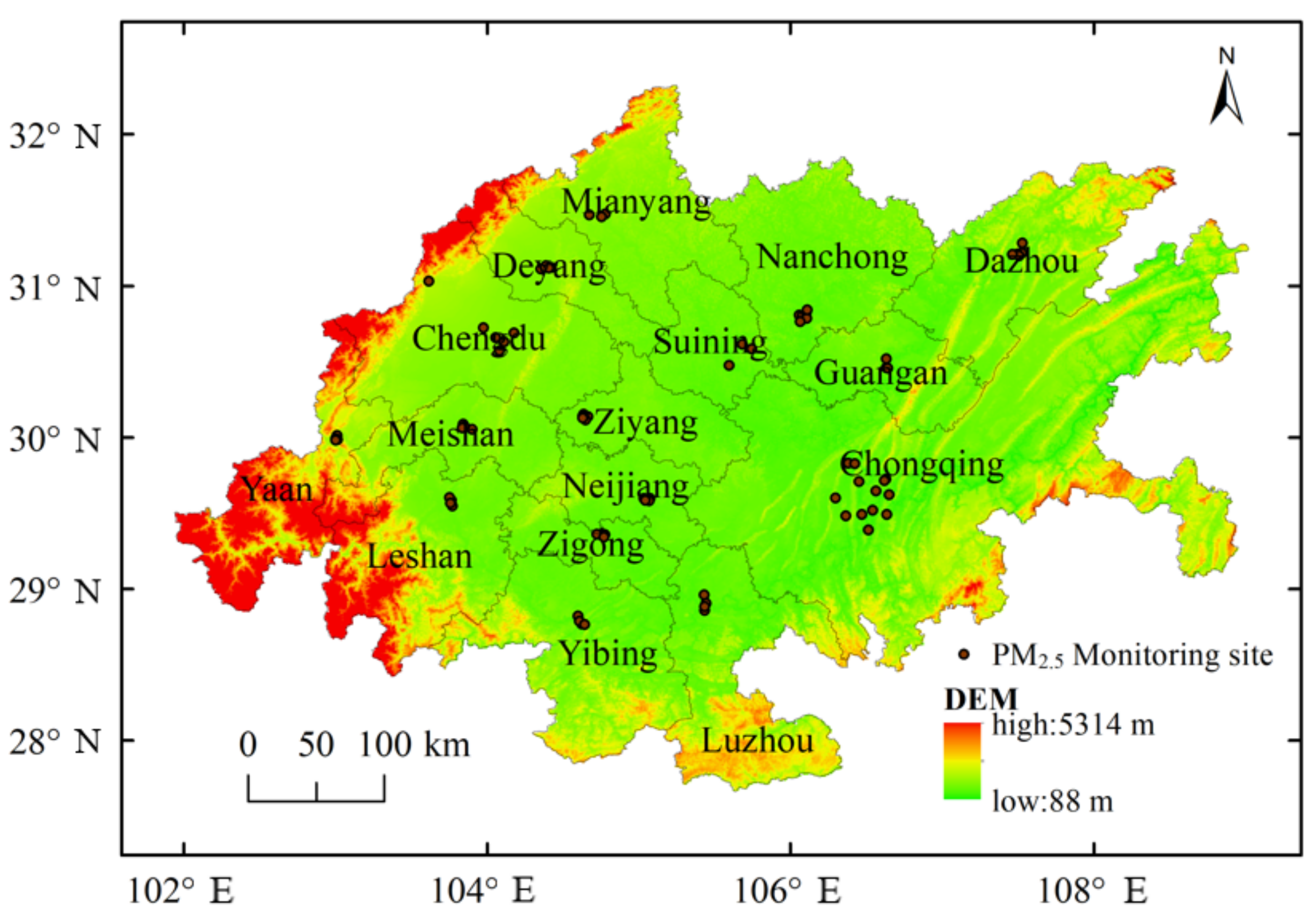
2.1. Research Area

The Chengdu Chongqing Economic Circle is located in the upper reaches of the Yangtze River, in the Sichuan Basin, connecting Shaanxi and Gansu in the north, Yunnan-Guizhou in the south, Qinghai Tibet in the west, and Hunan and Hubei in the east. The total area of 16 cities including Chengdu and Chongqing is 185,000 square kilometers (as shown in Figure 1). The region belongs to a subtropical monsoon climate, with high temperatures, rainy summer, warm winter is located in the basin, with wet weather, mist, and less sunshine as seasonal characteristics. Air pollution is second only to Beijing Tianjin Hebei in the “three regions and ten clusters”, and it is classified into the key control area of the national “Air Pollution Prevention and Control Action Plan”. It is of great significance to better simulate the spatial distribution of air pollution in the Chengdu Chongqing Economic Circle to propose pollution prevention and control strategies.

2.2. Data and Processing

To better simulate the spatial distribution of PM_2.5 concentration in the Chengdu Chongqing Economic Circle in 2018, the selection of relevant driving factors is a key step. The driving factors considered in most studies are mainly natural environmental factors and human activity intensity factors [26,27]. According to the commonly used geographically related variables affecting PM_2.5 and considering the actual situation in the region, the natural environmental factors selected in this study mainly involve meteorological factors, elevation, and vegetation coverage (AOD, WIN, PRES, TEM, SHUM, PREC, PBLH, DEM and NDVI). Human activity intensity factors include population density, night light, road traffic, and land use (POP, NL, WAY, LU). See

Table 1. Data sources for drivers.

Type	Name	English Abbreviations	Unit	Year	Spatial Resolution	Source
PM2.5 Monitoring data	Environmental monitoring station data	PM2.5	ug·m−3	2018	-	http://www.cnemc.cn/ (accessed on 10 December 2021)
Natural environmental factors	Aerosol Optical Depth	AOD	-	2018	1 km	https://ladsweb.modaps.eosdis.nasa.gov/ (accessed on 20 December 2021)
	Wind speed	WIN	m·s−1	2018	0.1° × 0.1°	http://data.tpdc.ac.cn/zh-hans/data/ (accessed on 20 December 2021)
	Pressure	PRES	hPa	2018
	Temperature	TEM	K	2018
	air humidity ratio	SHUM	-	2018
	Precipitation	PREC	mm	2018
	Planetary Boundary Layer Height	PBLH	m	2018	0.25° × 0.3°	ftp://rain.ucis.dal.ca/ctm/ (accessed on 20 December 2021)
	Digital Elevation Model	DEM	m	2018	90 m	http://www.gscloud.cn/search (accessed on 20 December 2021)
	Normalized Difference Vegetation Index	NDVI	%	2018	1 km	Data Center for Resources and Environmental Sciences, Chinese Academy of Sciences (https://www.resdc.cn) (accessed on 20 December 2021)
Human activity intensity factor	population density	POP	-	2018	100 m	World pop https://www.worldpop.org (accessed on 28 December 2021)
	Night light	NL	-	2018	1.5 km	http://satsee.radi.ac.cn/cfimage/nightlight (accessed on 28 December 2021)
	Road way	WAY	-	2018	-	http://www.openstreetmap.org (accessed on 28 December 2021)
	Land use	LU	-	2010	30 m	http://www.globallandcover.com (accessed on 28 December 2021)

for specific driving factors.

PM_2.5 monitoring data were obtained from the hourly value and the 24 h average value of PM_2.5 concentration of monitoring stations in Economic Circle in 2018 and downloaded from China Environmental Monitoring Center (http://www.cnemc.cn/) (accessed on 10 December 2021). The monthly average concentration of PM_2.5 was obtained by adding and averaging the average daily concentrations. There are 88 environmental monitoring stations in Chengdu–Chongqing Economic Circle. After screening, 76 environmental monitoring stations with 912 (12 × 76) groups of valid data were obtained.

AOD data is to use MCD19A2 V6 product (https://ladsweb.modaps.eosdis.NASA.Gov) (accessed on 20 December 2021), it is the secondary product of multi-angle Atmospheric Correction (MAIAC) land Aerosol optical depth (AOD) gridding combined with MODIS Terra and Aqua with a spatial resolution of 1 km [20]. Through GEE programming, the MCD19A2 V6 data products were trimmed and revamped into monthly 1 km AOD data in 2018 according to the vector layer of the Economic Circle, and then the missing value data were filled by the adjacent raster method combined with ArcGIS to obtain high-resolution AOD data sets.

Meteorological data from the national data center (http://data.tpdc.ac.cn/zh-hans/data/) (accessed on 20 December 2021) of the Qinghai Tibet plateau, including wind speed (WIN), temperature (TEM), air humidity ratio (SHUM), surface pressure (PRES), and Precipitation (PREC) data, the daily average of 2018 with a horizontal spatial resolution of 0.1 × 0.1° [26], were obtained, and the daily average is added and averaged to obtain the corresponding monthly average. The planetary boundary layer height was obtained from (ftp://rain.ucis.dal.ca/ctm/) (accessed on 20 December 2021), for data integration with a meteorological data by cutting, re-sampling into the same as the AOD data resolution (1 km × 1 km) and the same projected coordinate system (WGS84) raster data.

The intensity of human activities mainly considers the factors related to economic development and extremely frequent human activities. Population density data were obtained from the World of pop (https://www.worldpop.org) (accessed on 28 December 2021), the night light data were obtained from China academy of sciences, China remote sensing satellite ground station Chen Fu team (http://satsee.radi.ac.cn/cfimage/nightlight) (accessed on 28 December 2021). Elevation data (DEM) of the data were obtained from the geographical spatial data cloud (http://www.gscloud.cn/search) (accessed on 28 December 2021) using SRTM world 90 m resolution terrain elevation data representation. Land use data were obtained from a 30 m global surface coverage information service system (http://www.globallandcover.com) (accessed on 28 December 2021) with the spatial resolution of 30 m. Monthly vegetation coverage (NDVI) was obtained from the Data Center for Resources and Environmental Sciences, Chinese Academy of Sciences (https://www.resdc.cn) (accessed on 28 December 2021). PM_2.5 ground monitoring stations were used as the center of human activity intensity data to make buffer zones with different radii (0.5 km, 1 km, 2 km), and the buffer data with the greatest correlation coefficient with PM_2.5 concentration was selected as the influencing factor. Finally, the proportion of human activity intensity data in the buffer zone with a radius of 1 km, centered on the PM_2.5 ground monitoring station, was selected to represent the impact on PM_2.5 concentration. For example, NL calculates the average night light intensity in the buffer zone by partition statistics; WAY is the road length in the statistical buffer through spatial overlay analysis, which represents the road traffic condition [25]. LU represents the landuse status by the proportion of landuse types in the statistical buffer zone through the histogram in ArcGIS 10.7.

Next, the drivers need data fusion. Firstly, the data from a variety of different data sources should be matched, and the consistency of time and space should be maintained to ensure that all the data are in the same projection coordinate system (WGS84) and have the same resolution (1 km × 1 km). Then, the “raster extraction to the point” tool in ArcGIS 10.7 was used to obtain the monthly average natural environmental factor data corresponding to the monthly average PM_2.5 station data. Then, the human activity intensity factors were used as buffers with different radii centered on the PM_2.5 monitoring site, and the buffer data with the greatest correlation coefficient with PM_2.5 concentration was selected. Finally, a total of 912 sets of data from January to December 2018 were obtained, which were used to construct the model.

2.3. Research Methods

2.3.1. Model Principles

He and Huang [28] proposed the GTWR model based on the GWR model. The regression parameters of the independent variables in the GWR model changed with the change in spatial and geographic location, while the regression parameters of the independent variables in the GTWR model changed with the change in spatiotemporal location. Therefore, compared with the GWR model, this model can better describe the spatiotemporal relationship between explanatory variables and dependent variables. The basic expression of the GTWR model is as follows:

$$y_i={\beta }_0\left({\mu }_i, v_i, t_i\right)+{\displaystyle \sum }_{k=1}^m{\beta }_k\left({\mu }_i, v_i, t_i\right)X_{ik}+{\epsilon }_i$$

(1)

In the above expressions, (${\mu }_i$, $v_i$) represents the longitude and latitude coordinates of the ith sample point, $t_i$ represents the observation time, ${\beta }_k$ represents the dependent variable value of the kth and $X_{ik}$ represents the kth explanatory variable of the ith sample point. ${\epsilon }_i$ is the model error term, ${\beta }_0$ (${\mu }_i$, $v_i$, $t_i$) represents the regression constant of the ith sample point, and ${\beta }_k$ (${\mu }_i$, $v_i$, $t_i$) represents the regression coefficient of the kth explanatory variable of the ith sample point.

XGBoost model, the full name of which is eXtreme Gradient Boosting, is an optimized distributed Gradient Boosting library designed to be efficient, flexible, and portable. XGBoost is an additive model composed of k-basis models to obtain better regression results than those of a single model. The idea of XGBoost is to add trees continuously. Each time a tree you add, a new function F you learn to fit the residual of the last prediction. After training, k trees you get, each tree will fall to a correspond leaf node, and each leaf corresponds to a score. Assuming that the model has a total of k trees, the prediction result of the whole model on the sample $i$ is shown in Equation (2).

$$\widehat{y_i}={\displaystyle \sum }_{k=1}^K{f}_k\left(x_i\right),$$

(2)

where $\widehat{y_i}$ is the final predicted score of $x_i$, $f_k$ is the leaf score mapping of the kth tree, and $x_i$ is the corresponding feature variable of the sample.

2.3.2. Variable Screening

Natural environmental factors were extracted from the above processed data set. Spearman correlation analysis was used to test the correlation between each natural environmental factor variable and PM_2.5 monitoring data. Not all natural environmental factor variables with significant correlation are suitable for the modeling prediction of the GTWR model in Stage 1. The variance inflation factor (VIF) is used to check the collinearity of variables in the model. The natural environment factor variables with VIF > 4 are eliminated, and the variables with VIF ≤ 4 are input into the GTWR model [29,30]. The results are shown in

Table 2. Correlation coefficient and collinearity test between each variable and PM_2.5 concentration.

Variable	Correlation Coefficient	VIF Value
AOD	0.32	1.17
WIN	−0.06	2.36
PRES	0.20	3.12
TEM	−0.77	14.74
SHUM	−0.77	18.09
PREC	−0.65	2.68
PBLH	−0.70	2.11
DEM	−0.04	6.46
NDVI	−0.50	2.96

. The previous data has not been standardized, because spatiotemporal geographical weighted regression can be used to build regression equations to predict PM_2.5 concentration through raw data.

The correlation coefficient in Table 2 shows that AOD and PRES are positively correlated with PM_2.5 concentration, while TEM, SHUM, PREC, PBLH, and NDVI are negatively correlated with PM_2.5 concentration. As can be seen from the VIF values in Table 2, TEM, SHUM, and DEM show serious multicollinearity, and the VIF values are all less than 4 after removing TEM, SHUM, and DEM by stepwise regression. Therefore, all the variables meeting the conditions can be added to the GTWR model to obtain the PM_2.5 concentration with information. Then, TEM, SHUM, DEM, and the human activity intensity factors in the buffer zone with the best correlation coefficient of PM_2.5 were incorporated into XGBoost machine learning in the second stage (Stage 2). Because machine learning can better describe the complex nonlinear relationship between influencing factors and PM_2.5, without considering the multicollinearity problem among variables, it can be incorporated into the machine learning model to obtain the predicted value of PM_2.5.

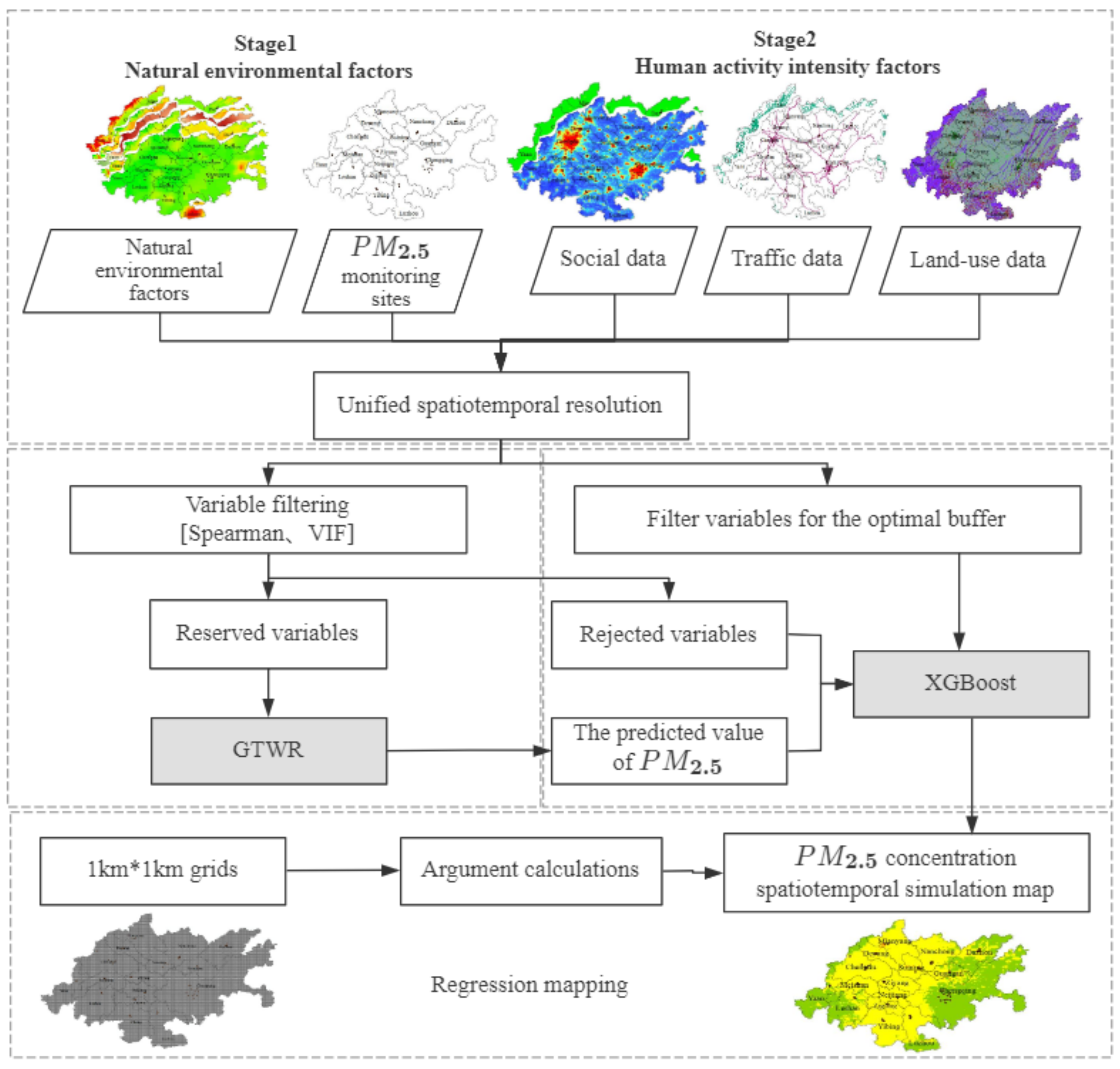
2.3.3. Two-Stage Model Construction and Experimental Scheme Design

The modeling of the GTWR-XGBoost model is divided into two stages. The first stage is to unify the spatiotemporal resolution of natural environmental factors and PM_2.5 monitoring site data, and then screen out the variables suitable for the GTWR model through variable screening and variance inflation factor. The concentration of GTWR_{PM_2.5} with spatiotemporal characteristics was obtained by putting it into the GTWR model. In the second stage, the concentration of GTWR_{PM_2.5}, the human activity intensity factors in the buffer zone with the best correlation coefficient of PM_2.5, and the excluded variables that are not suitable for the GTWR model were incorporated into XGBoost machine learning. The XGBoost machine learning model is used to learn the complex nonlinear relationship between the influencing factors of PM_2.5 and the optimal model is obtained. Finally, the area was divided into a 1 km × 1 km grid, and the independent variable data of the grid unit were obtained. The optimal model calculated the simulation diagram of monthly, quarterly, and annual PM_2.5 concentration spatiotemporal distribution in the Chengdu–Chongqing area in 2018 [21]. The two stages can effectively avoid the defects of a single model. The GTWR model is difficult to describe complex nonlinear relationships and the XGBoost model lacks consideration of heterogeneity. The technical route of the GTWR-XGBoost model is shown in Figure 2.

After establishing the geographically weighted regression model combined with the XGBoost model to obtain the optimal accuracy, the model was saved, and then the corresponding independent variable values on the grid were obtained. The predicted values of PM_2.5 concentration in grid points were obtained through model calculation, and the distribution simulation map of monthly, quarterly, and annual PM_2.5 concentration in the area in 2018 was generated [21].

When setting the comparison model, the ablation experiment is firstly performed to reflect the advantages and disadvantages of the prediction results of the improved two-stage model. The first scheme is only considering the influence of natural environment factors on PM_2.5 concentration, which will only join into a single model to simulate the natural environment factors (such as Table 3), the second way is by the natural environment and human activity intensity factors through the screening of variables, all to join a single model simulated (Table 4), and the third way with the improved model of two phases, the natural environmental factors were screened and added to the spatiotemporal geographic weighted regression model. Then, the PM_2.5 variables obtained from spatiotemporal information combined with landuse data were added to the machine learning model for simulation. In addition, comparisons were made with recent literature on PM_2.5 inversion concentration, such as LUR-RF [21], LUR-XGBoost [29], STRF [20], and STXGBoost [31] schemes (see Table 5). In the second stage, the maximum depth of parameters used by XGBoost is 4, the maximum number of iterations is 301, and the iteration step is 0.25. Software: ArcGIS 10.7, Pycharm 2020.2, Python 3.0, NumPy 1.17.3, Pandas 1.1.3; Hardware: i5 processor lntel(R) Core(TM), 16 GB RAM, 500 GB SSD.

Table 3. A single model that considers only natural environmental factors.

Model	Cross-Validation			Forecast Validation
	R2	RMSE/ug·m−3	MAE/ug·m−3	R2	RMSE/ug·m−3	MAE/ug·m−3
LUR	0.68	10.72	8.06	0.63	11.16	8.55
GTWR	0.82	7.65	5.42	0.78	8.64	5.82
RF	0.80	8.49	6.33	0.75	9.28	6.74
XGBoost	0.87	6.73	4.97	0.87	6.56	4.75

Table 3. A single model that considers only natural environmental factors.

Model	Cross-Validation			Forecast Validation
	R2	RMSE/ug·m−3	MAE/ug·m−3	R2	RMSE/ug·m−3	MAE/ug·m−3
LUR	0.68	10.72	8.06	0.63	11.16	8.55
GTWR	0.82	7.65	5.42	0.78	8.64	5.82
RF	0.80	8.49	6.33	0.75	9.28	6.74
XGBoost	0.87	6.73	4.97	0.87	6.56	4.75

Table 4. The overall model considers the factors of the natural environment and human activity intensity.

Model	Cross-Validation			Forecast Validation
	R2	RMSE/ug·m−3	MAE/u ug·m−3	R2	RMSE·ug/m−3	MAE/ug·m−3
LUR	0.71	10.24	7.60	0.69	10.29	7.80
RF	0.84	8.23	6.11	0.80	8.24	6.11
GTWR	0.78	7.86	7.22	0.76	8.86	6.68
XGBoost	0.91	5.60	4.23	0.90	5.59	3.99

Table 4. The overall model considers the factors of the natural environment and human activity intensity.

Model	Cross-Validation			Forecast Validation
	R2	RMSE/ug·m−3	MAE/u ug·m−3	R2	RMSE·ug/m−3	MAE/ug·m−3
LUR	0.71	10.24	7.60	0.69	10.29	7.80
RF	0.84	8.23	6.11	0.80	8.24	6.11
GTWR	0.78	7.86	7.22	0.76	8.86	6.68
XGBoost	0.91	5.60	4.23	0.90	5.59	3.99

Table 5. This model is compared with recent research models.

Model	Cross-Validation			Forecast Validation
	R2	RMSE/ug·m−3	MAE/ug·m−3	R2	RMSE/ug·m−3	MAE/ug·m−3
STXGBoost [31]	0.90	5.86	4.39	0.88	6.32	4.33
STRF [20]	0.81	8.12	6.08	0.78	8.77	6.42
LUR-RF [21]	0.82	7.85	5.92	0.78	8.76	6.52
LUR-XGBoost [29]	0.90	5.99	4.63	0.87	6.60	4.81
GTWR-LUR	0.85	7.24	5.50	0.82	7.81	5.72
GTWR-RF	0.86	7.15	5.30	0.84	7.31	5.57
GTWR-XGBoost	0.92	5.44	4.12	0.93	4.75	3.42

Table 5. This model is compared with recent research models.

Model	Cross-Validation			Forecast Validation
	R2	RMSE/ug·m−3	MAE/ug·m−3	R2	RMSE/ug·m−3	MAE/ug·m−3
STXGBoost [31]	0.90	5.86	4.39	0.88	6.32	4.33
STRF [20]	0.81	8.12	6.08	0.78	8.77	6.42
LUR-RF [21]	0.82	7.85	5.92	0.78	8.76	6.52
LUR-XGBoost [29]	0.90	5.99	4.63	0.87	6.60	4.81
GTWR-LUR	0.85	7.24	5.50	0.82	7.81	5.72
GTWR-RF	0.86	7.15	5.30	0.84	7.31	5.57
GTWR-XGBoost	0.92	5.44	4.12	0.93	4.75	3.42

2.3.4. Accuracy Verification

The evaluation indexes used in this paper include the coefficient of determination (R²), root mean square error (RMSE), and mean absolute error (MAE). The model fitting is based on the same data set, which cannot reflect whether there is an over-fitting phenomenon in the model. Therefore, the 10-fold cross-validation (CV) method [31] was used to test the prediction accuracy of the model. Among the above indicators, R² reflects the fitting effect of the model whose value ranges from 0 to 1. The larger R² indicates the better fitting effect; RMSE and MAE reflect the deviation between the predicted value and the real value, and the smaller value indicates better model accuracy [20,29].

$$R^2=1-\frac{{{\displaystyle \sum }}_{i=1}^n{\left(y_i-\widehat{y}\right)}^2}{{{\displaystyle \sum }}_{i=1}^n{\left(y_i-\overline{y}\right)}^2},$$

(3)

$$RMSE=\sqrt{\frac{{{\displaystyle \sum }}_{i=1}^n{(y_i-\widehat{y})}^2}{n-1}},$$

(4)

$$MAE=\frac{ {{\displaystyle \sum }}_{i=1}^n\left|y_i-\widehat{y}\right|}{n},$$

(5)

where $y_i$ is the actual observed value, $\widehat{y}$ is the predicted value, $\overline{y}$ is the average value of the observed value, and n is the number of predicted samples.

3. Results and Analysis

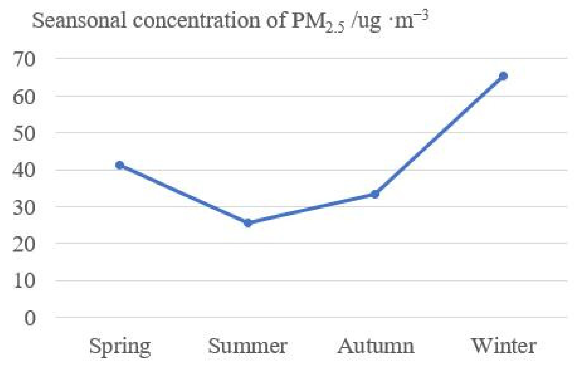
3.1. Statistical Results

The statistical results of the natural environment variables involved in the model (AOD, WIN, PRES, TEM, SHUM, PREC, PBLH, DEM, and NDVI) are shown in

Table 6. Statistical results of the natural environment variables.

Variable	Average	Minimum	Maximum	Standard Deviation
PM2.5/ug m−3	41.38	4.99	112.43	18.95
WIN/m s−1	1.89	1.06	3.49	0.46
TEM/K	290.99	274.54	305.23	7.5
SHUM	0.018	0	0.03	0
PRES/hPa	96,337.89	85,962	99,940	2333.02
PREC/mm	0.18	0	0.79	0.12
AOD	618.88	0	1798.25	433.43
PBLH/m	674.61	296.48	892.52	168.89
NDVI	0.38	0.018	0.888	0.17
dem/m	390.33	199	1346	147.16

. The average concentration of PM_2.5 was 41.38 ug·m⁻³, mainly distributed in the range of 4.99~112.42 ug·m⁻³, and the standard deviation was 18.95 ug·m⁻³. Aerosol optical depth (AOD) is a key physical quantity to characterize the degree of atmospheric turbidity and an important factor to determine the aerosol climate effect. Its average value was 618.88, the standard deviation was 433.43. Wind speed (WIN) ranged from 1.06 to 3.49 m·s⁻¹, with a standard deviation of 0.46 m·s⁻¹. It had a small range of variation compared to other variables. Atmospheric pressure (PRES) mainly affects the stability of the atmosphere, the average value is 96337.89 Pa, and the standard deviation is 2333.02 Pa. Temperature (TEM) mainly affects atmospheric mobility, with a mean value of 290.99 K and a standard deviation of 7.5 K. The mean value of relative humidity (SHUM) is 1.8%, and the standard deviation is 0%, indicating that the atmosphere in 2018 was basically humid. Precipitation (PREC) ranged from 0 to 0.79 mm, with an average of 0.18 mm. Planetary boundary layer height (PBLH) can affect the vertical distribution of PM_2.5. Its minimum value was 296.48 m, its maximum value is 674.61 m, and its standard deviation was 168.89 m. Normalized difference vegetation index (NDVI) can reduce the concentration of PM_2.5. Its minimum value is 0.018, its maximum value is 0.888, the standard deviation is 0.12. Digital elevation model (DEM) mainly affects the concentration of PM_2.5, with a minimum of 199 m and a maximum of 1346 m.

3.2. Model Comparison and Analysis

In this method, the dataset was randomly divided into 10 groups: 9 groups were used for model fitting, and the remaining 1 group was used for validation. This process was repeated 10 times until each group of data was validated once. The R², RMSE, and MAE after CV were calculated to evaluate the accuracy of the model. As can be seen from Table 3, through cross-validation and prediction validation, R² of XGBoost machine learning cross-validation reaches 0.87, which is significantly higher than LUR, GTWR, and RF, indicating that XGBoost machine learning can better express the complex nonlinear relationship between meteorological factors and PM_2.5. However, compared with LUR and RF, the simulation effect of GTWR is better, indicating that the inversion accuracy of PM_2.5 considering spatial and temporal heterogeneity is improved. By comparing the data in Table 3 and Table 4, it can be seen that considering more influencing factors of PM_2.5 can improve the accuracy of simulation to a certain extent, and can better describe the complex nonlinear relationship between predictors and PM_2.5. In particular, the R² of XGBoost cross-validation was increased by 0.02. RMSE decreased from 6.73 ug·m⁻³ to 5.60 ug·m⁻³, MAE decreased from 4.97 ug·m⁻³ to 4.23 ug·m⁻³, but the cross-validation results of GTWR decreased, because GTWR is a statistical regression model which cannot learn the complex nonlinear relationship well, resulting in a decrease in the prediction accuracy among multiple variables. As can be seen in Table 5, the cross-validation and predictive validation of the proposed model were both better than those of the recent research model, with R² of 0.92, RMSE and MAE of 5.44 ug·m⁻³ and 4.12 ug·m⁻³, respectively. Compared with the recent spatiotemporal coupling model, R² was increased by 0.02, and MAE was reduced by more than 0.4. GTWR-XGBoost can well express the improvement of model performance caused by considering spatiotemporal heterogeneity and complex nonlinear relationships.

To compare the model accuracy, on the premise of ensuring the same independent variables, this paper constructed the fitting scatter plot of the corresponding PM_2.5 predicted concentration and ground monitored concentration, as shown in Figure 3 below. Figure 3 shows the scatter density maps fitted between the PM_2.5 concentrations estimated by STXGBoost, STRF, LUR-RF, LUR-XGBoost, GTWR-LUR, GTWR-RF, and GTWR-XGBoost models and the PM_2.5 concentrations measured at ground monitoring stations. It can be seen from Figure 3 that the GTWR-XGBoost model is superior to STXGBoost and STRF models, and the cross-validation R², RMSE, and MAE were 0.92, 5.44 ug·m⁻³, and 4.12 ug·m⁻³, respectively. Firstly, the GTWR model can better learn the spatiotemporal correlation of PM_2.5 monitoring site data to describe the spatiotemporal characteristics and then combine the factors of human activity intensity to express the complex nonlinear relationship of PM_2.5 concentration, which improves the accuracy of PM_2.5 estimation. The second is the accuracy of LUR-XGBoost model. By screening variables of various influencing factors of PM_2.5 through LUR, the factors with low influence can be effectively excluded. At the same time, the spatial correlation of site data can be obtained by combining Kring interpolation method to retrieve PM_2.5, which can obtain better accuracy. The STRF model had the worst effect on the estimation of ground PM_2.5 concentration. The cross-validation R², RMSE and MAE were 0.81, 8.12 ug·m⁻³ and 6.08 ug·m⁻³, respectively.

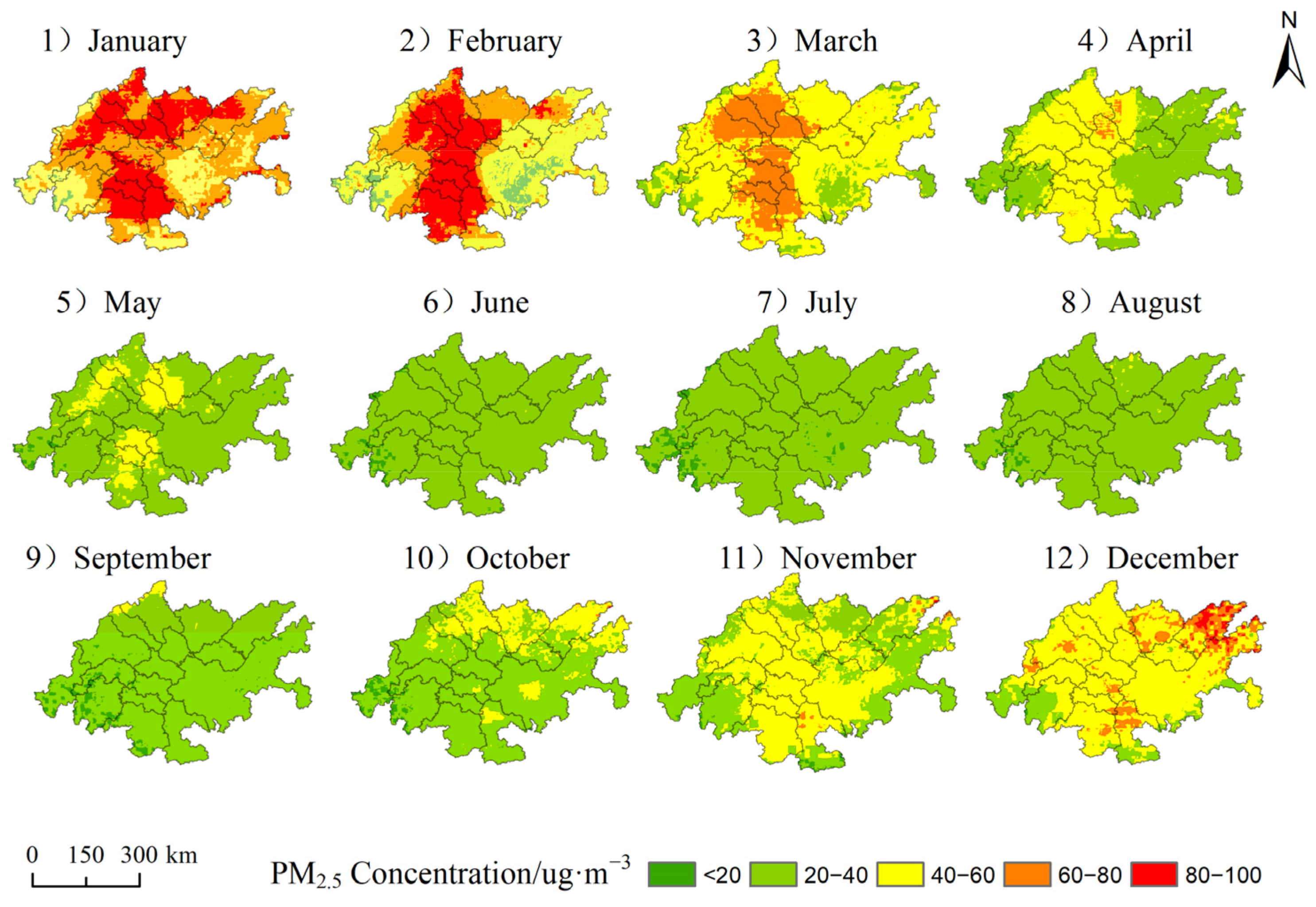
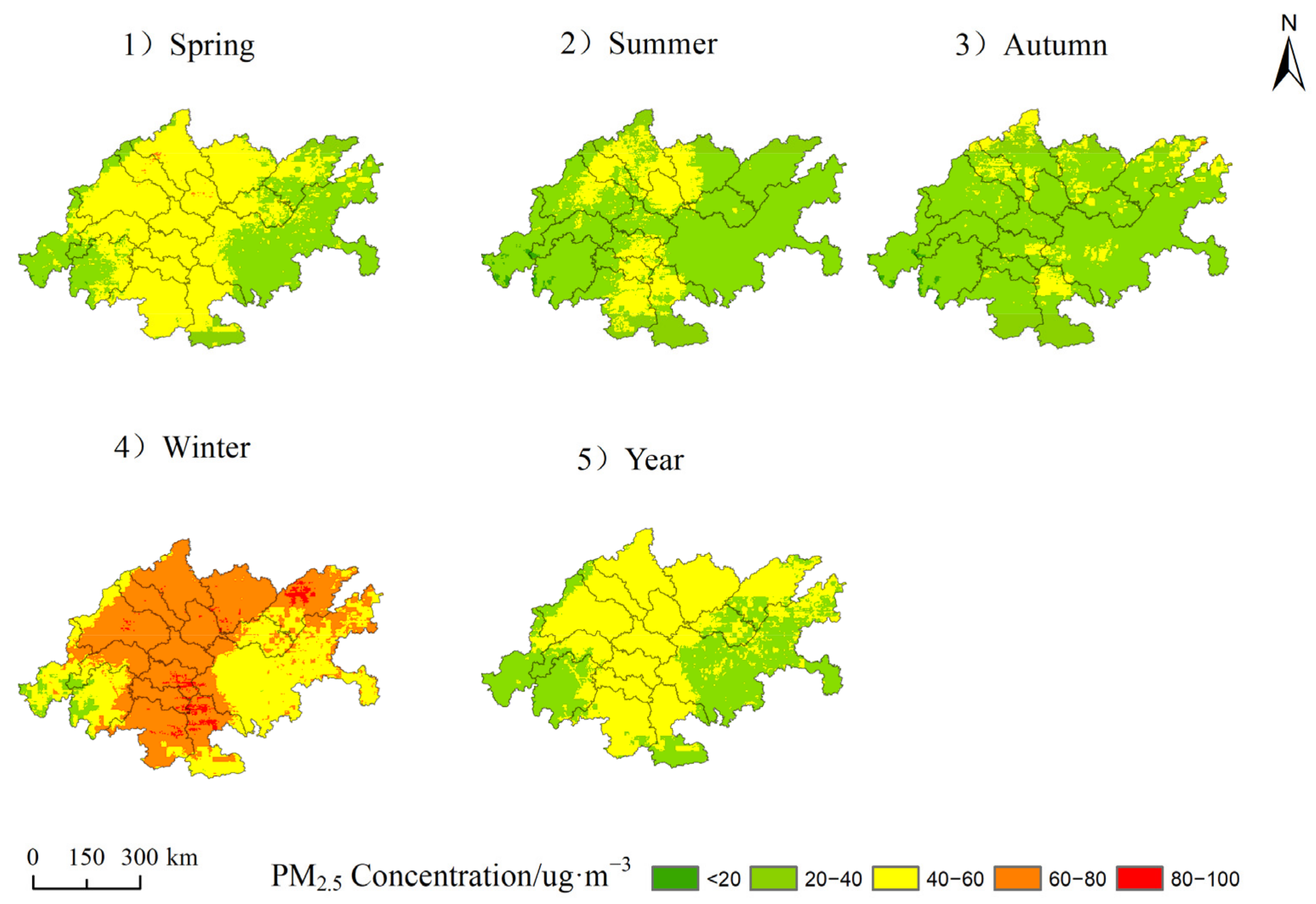
3.3. Spatiotemporal Distribution of PM_2.5 Concentration in the Region

The temporal variation of PM_2.5 concentration includes daily, monthly, quarterly and inter-annual variations. The time scales studied in this paper are month, season, and year. From the perspective of monthly variation, taking 2018 as an example, the variation of monthly average PM_2.5 concentration in the area generally decreased first and then increased, showing a V-shaped pattern. In January and February, the pollution was the most serious, with an average value of 69.90 ug·m⁻³ and 69.88 ug ·m⁻³, respectively. Secondly, in March, November and December the average value exceeded 40 ug·m⁻³. The average value was 20.28 ug·m⁻³ in September. PM_2.5 decreased from 69.90 ug·m⁻³ in January to 21.12 ug ·m^-3 in July. Increased from 20.28 ug·m⁻³ in September to 56.38 ug·m⁻³ in December. The seasonal variation of PM_2.5 in the region is obvious. Statistics show that the average values of spring (3, 4, 5), summer (6, 7, 8), autumn (9, 10, 11), and winter (12, 1, 2) in this region are 41.19 ug ·m⁻³, 25.58 ug·m⁻³, 33.40 ug·m⁻³, 65.34 ug·m⁻³, respectively (as shown in Figure 4), in which the values of winter and spring is 1.8 times that of summer and autumn. The seasonal variation of PM_2.5 concentration was roughly consistent with the monthly trend, with winter > spring > autumn > summer.

When analyzing the long-term time series trend of PM_2.5 concentration, the annual average variation of PM_2.5 concentration can be increased to observe the variation trend of perennial PM_2.5 concentration. After the national air protection measures, PM_2.5 concentration has decreased year by year, indicating that human activities strongly control the trend of overall PM_2.5 concentration.

From the perspective of spatial variation (as shown in Figure 5), PM_2.5 in is characterized by high, middle and low concentrations on both sides, with high local pollution. High pollution accumulation areas are mainly distributed in Chengdu, Deyang, Mianyang, Suining, Ziyang, Neijiang, Zigong, Yibin, and other regions. The main reason is that the eastern part of Sichuan is more developed in industry, automobile exhaust, human activities and other emissions of the PM_2.5 concentration is high. Secondly, Sichuan is a basin on the landform, Chengdu is a plain, and Chongqing is blocked by mountains [32], which is not conducive to the diffusion of PM_2.5. Finally, in winter, in region, the southeasterly wind combined with the terrain may present a phenomenon of PM_2.5 gathering in the southeast region. Meishan, Leshan, and Ya’an in the west of Chengdu and Chongqing, as well as Chengkou and Wuxi in the east of Chongqing, have fewer human activities, less pollutant emissions, and higher vegetation coverage, which has a strong effect on pollutant cleaning.

The spatial distribution of PM_2.5 concentration has an obvious seasonal variation (as shown in Figure 6). In spring (35.86~48.69 ug·m⁻³), the high pollution was mainly concentrated in Chengdu, Deyang, Mianyang, Suining, Nanchong, Ziyang, Neijiang, Zigong, Yibin, Luzhou, and in the west of Chongqing, while the low pollution was mainly in Yaan, Leshan, Dazhou, southern Luzhou and in the east of Chongqing. In summer (21.12~29.48 ug·m⁻³), the area is a low-pollution area due to three reasons. First, the high temperature in summer is conducive to formation of strong convective weather, which is in turn conducive to the diffusion of PM_2.5. Second, the vegetation coverage rate is high, and there is a strong purification of air pollutants. Third, due to high precipitation and high air humidity, ground dust is not easy to diffused [33]. In autumn (20.28~46.26 ug·m⁻³), compared with summer, the concentration of PM_2.5 increased significantly, mainly distributed in the northern part of Luzhou, the eastern part of Neijiang, the central part of Deyang, the northern part of Mianyang, the southern part of Nanchong and the northeastern part of Dazhou. The increase in pollution concentration was mainly caused by industry, manufacturing, and thermal power generation [27]. In winter (56.38~69.90 ug·m⁻³), high pollution is mainly distributed in Chengdu plain and the southern Sichuan Economic Zone. The reason is that the region is located in a basin and receives less solar radiation in winter, which is not conducive to the diffusion of air pollution. In addition, there is more heating, greater emission and combustion pollution, more rain, and less wind, which is not convenient for air circulation.

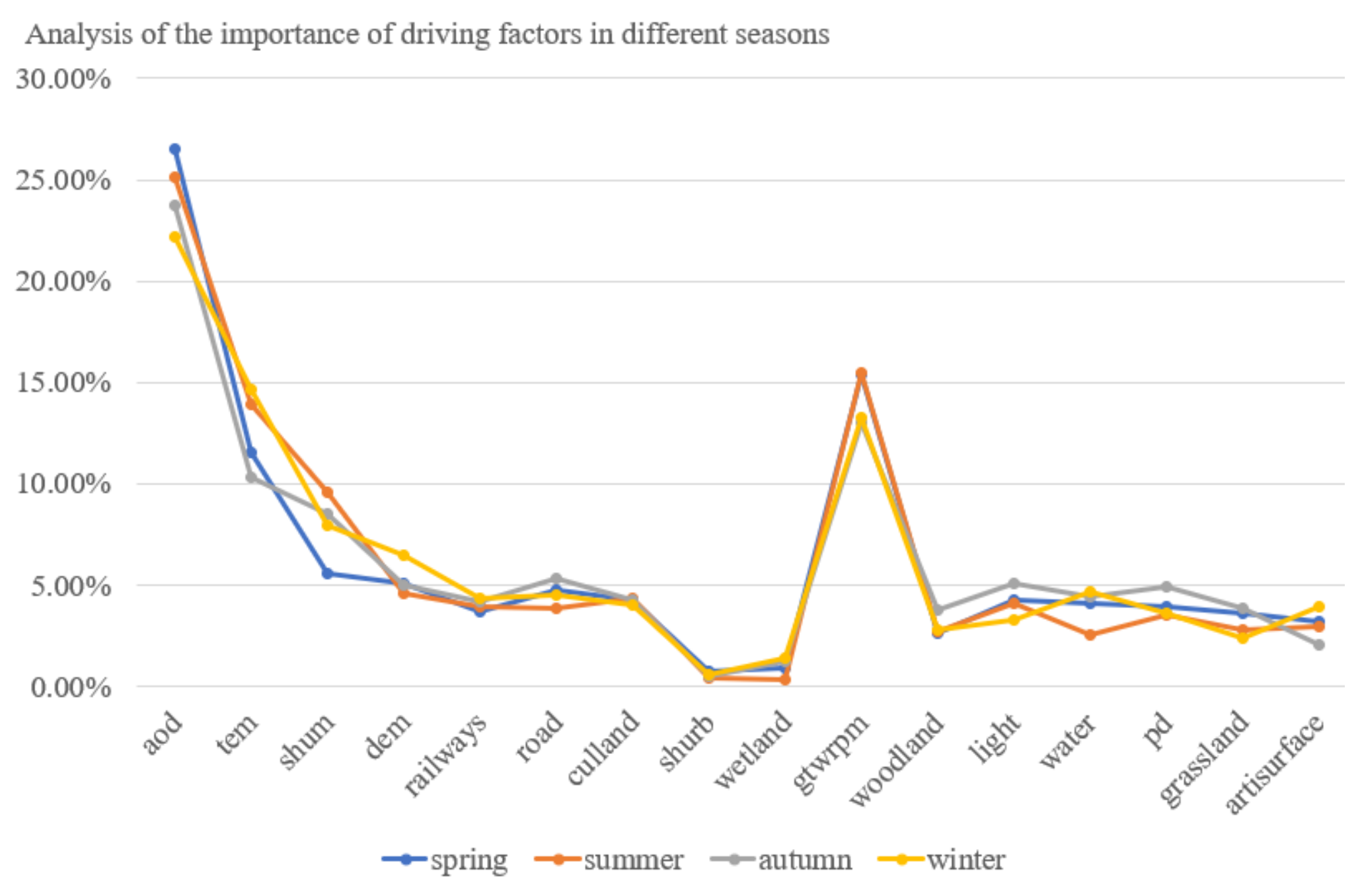
3.4. Analysis of Influencing Factors

The correlation between PM_2.5 and the selected variables was analyzed at the monthly scale. The results showed that AOD and PRES were positively correlated with PM_2.5 concentration, while TEM, SHUM, PREC, PBLH and NDVI were negatively correlated with PM_2.5 concentration. TEM, SHUM, PRES, PREC, AOD, PBLH and NDVI were important influencing factors, and the correlation coefficients were −0.77, −0.77, 0.20, −0.65, 0.32, −0.70, and 0.50, respectively.

According to the analysis of the importance of driving factors in different seasons (as shown in Figure 7), the proportions of AOD, GTWR_{PM_2.5}, TEM, and SHUM to PM_2.5 concentration was about 23%, 17%, 14%, and 12%, respectively, and their importance decreased successively, indicating that meteorological factors have a greater impact on the retrieval of PM_2.5, with a contribution rate of 66%. All the selected human activity intensity factors contribute 34% to the retrieval of PM_2.5 concentration, among which the cultivated land (culland), road, railway, Artificial surface (artisurface), population density (PD), and night light (NL) had moderate impacts on PM_2.5, contribute 20% to the retrieval of PM_2.5 concentration, the forest land, grassland, wetland, shrub, and water contribution the inversion of PM_2.5 concentration is the lowest.

According to the statistics of the data, natural causes are dominant, but the intensity of the effect of human causes on PM_2.5 can be seen from the change in the total amount of PM_2.5 over a long period of time.

Although machine learning modeling does not represent a causal relationship, it largely reflects the influence of natural and human factors on the spatiotemporal distribution of PM_2.5 concentration. Natural factors affect the spatiotemporal patterns of PM_2.5 in a relatively static and passive manner. However, human factors mostly affect the spatiotemporal pattern of PM_2.5 in a dynamic and active way. They interact with each other and form the spatiotemporal pattern of PM_2.5 concentration in a region.

4. Conclusions and Discussion

In this paper, a two-stage sequential hybrid model is proposed, which can not only describe the heterogeneity of the phenomenon and reveal the complex nonlinear relationship between the phenomenon and the influencing factors, but also separate the natural environmental factors and human factors that affect the concentration of PM_2.5. This model not only improves the performance but also enhances its interpretability of the model.

In the first stage of the mixed model, the natural environmental factors were used to screen the driving factors, and Geographically and Temporally Weighted Regression (GTWR) was used to predict the PM_2.5 concentration with spatiotemporal characteristics. In the second stage, the results obtained in the first stage were superimposed on the human activity intensity factors and the influencing factors that were not suitable for GTWR modeling. The data is used as the input of the XGBoost machine learning model to learn the complex nonlinear relationship between PM_2.5, and finally reverse the spatiotemporal distribution of PM_2.5.

By using the GTWR-XGBoost two-stage sequential model to learn and reason the PM_2.5 concentration of Economic Circle in 2018, the results show that R², RMSE, and MAE are 0.92, 5.44 ug·m⁻³ and 4.12 ug·m⁻³, respectively, using the cross-validation method. R², RMSE, and MAE were 0.93, 4.75, and 3.42 ug·m⁻³, respectively. The results show that the GTWR-XGBoost two-stage model outperforms the single GTWR, XGBoost, and recently published spatiotemporal coupling models in terms of simulation accuracy. The PM_2.5 concentration in Chengdu Chongqing Economic Circle has obvious spatiotemporal differentiation characteristics, and different driving factors have different forces. Natural environmental factors and human factors have 0.66 and 0.34 explanatory power, respectively, for the spatiotemporal distribution of PM_2.5 concentration. Among the three types of influencing factors, first, natural environmental factors are the most important, secondly, meteorological factors are the secondary factors, and AOD has the greatest impact on PM_2.5, finally, human factors have been the least important in recent years, which may be affected by meteorological factors, thus reducing the impact on PM_2.5 in some ways.

There are still some deficiencies in this paper. First of all, this paper tries to separate the natural environmental factors and human factors as much as possible and model them in stages. However, it is likely that the aerosol optical thickness and other factors in meteorological elements are caused by human factors and finally reflected by meteorological conditions. How human factors cause changes in climate conditions such as aerosol optical thickness is exactly the difficulty of analysis (this is not the focus of this paper). Therefore, to analyze the mechanism of natural environmental factors and human factors on the formation of PM_2.5 concentration, further research is needed later. Secondly, because the spatial resolution of the meteorological data used is 0.1°, the obtained meteorological data in the Chengdu Chongqing region is blocky, and higher resolution meteorological data can be used later to improve the situation. Finally, the results of GTWR-XGBoost model on monthly and seasonal scales are different. The reason may be that each independent variable has different contributions to the model in different months and seasons. Therefore, using different methods and different time scales to explore more reasonable combinations of variables to improve the model accuracy remains to be further studied.

References

1. Sundar, C.; Pawan, G. Global Distribution of Column Satellite Aerosol Optical Depth to Surface PM2.5 Relationships. Remote Sens. 2020, 12, 1985. [Google Scholar]
2. Cui, X. Prediction Model and Spatiotemporal Analysis of PM2.5 Concentration in Beijing-Tianjin-Hebei Region; Shandong University of Science and Technology: Qingdao, China, 2018. [Google Scholar]
3. Jing, Y.; Sun, Y.; Xu, H. Estimation of daily PM2.5 concentration in the Beijing-Tianjin-Hebei Region based on the mixed-effect model. China Environ. Sci. 2018, 38, 2890–2897. [Google Scholar]
4. Lee, H.J. Benefits of high-resolution PM2.5 prediction using satellite MAIAC AOD and land use regression for exposure assessment: California Examples. Environ. Sci. Technol. 2019, 53, 12774–12783. [Google Scholar] [CrossRef] [PubMed]
5. Liang, F.C.; Xiao, Q.Y.; Wang, Y.J. MAIAC-based long-term spatiotemporal trends of PM2.5 in Beijing, China. Sci. Total Environ. 2018, 616–617, 1589–1598. [Google Scholar] [CrossRef]
6. Zhao, B.; Liu, B. Estimation of ground PM2.5 concentration based on Stacking. Environ. Eng. 2020, 38, 153–159. [Google Scholar]
7. Wang, J.; Christopher, S.A. Intercomparison between satellite-derived aerosol optical thickness and PM2.5 mass: Implications for air quality studies. Geophys. Res. Lett. 2003, 30, 2095. [Google Scholar] [CrossRef]
8. Li, X.; Wu, S.; Xu, Y. Simulation of spatial-temporal variation pattern of PM2.5 mass concentration in Jiangsu province. Environ. Monitor. Manag. Technol. 2017, 29, 16–20. [Google Scholar]
9. Xu, G.; Jiao, L.; Xiao, F. Land use a regression model to simulate the spatial distribution of PM2.5 concentration in Beijing-Tianjin-Hebei. J. Arid Land Resour. Environ. 2016, 30, 116–120. [Google Scholar]
10. Yang, X.; Song, C.; Fan, L. Simulation and analysis of spatiotemporal variations of PM2.5 concentration in the Beijing-Tianjin-Hebei region. Environ. Sci. 2021, 42, 4083–4094. [Google Scholar]
11. Sun, C.; Wang, W.; Liu, F.T. Spatiotemporal variation of PM2.5 concentration in Hebei province based on linear mixed effects model. Environ. Sci. Res. 2019, 32, 1500–1509. [Google Scholar]
12. Fu, H.; Sun, Y.; Wang, B. Estimation of PM2.5 concentration in Beijing-Tianjin-Hebei Region based on AOD data and GWR model. China Environ. Sci. 2019, 39, 4530–4537. [Google Scholar]
13. Jia, H.; Luo, J.; Xiao, D. Spatiotemporal characteristics of PM2.5 concentration in Chengdu based on remote sensing data and GWR model. Chin. J. Atmos. Environ. Opt. 2021, 16, 529–540. [Google Scholar]
14. He, Q.; Huang, B. Satellite-based high-resolution PM2.5 estimation over the Beijing-Tianjin-Hebei region of China using an improved geographically and temporally weighted regression model. Environ. Pollut. 2018, 236, 1027–1037. [Google Scholar] [CrossRef]
15. Du, Z.; Wu, S.; Wang, Z. Estimation of spatial distribution of PM2.5 concentration in China based on weighted regression of geographical neural network. J. Geo-Inform. Sci. 2020, 22, 122–135. [Google Scholar]
16. Chen, B.; You, S.; Ye, Y. An interpretable self-adaptive deep neural network for estimating daily spatially-continuous PM2.5 concentrations across China. Sci. Total Environ. 2021, 768, 144724. [Google Scholar] [CrossRef]
17. Xia, X.; Chen, J.; Wang, J. Analysis of influencing factors of PM2.5 concentration in China based on random forest model. Environ. Sci. 2020, 41, 2057–2065. [Google Scholar]
18. Liu, L.; Zhang, Y.; Li, Y. Remote sensing retrieval of PM2.5 concentration in east China based on deep learning. Environ. Sci. 2020, 41, 1513–1519. [Google Scholar]
19. Kang, J.F.; Huang, L.X.; Zhang, C.Y. Prediction and Comparative Analysis of Hourly PM2.5 in Multi-Machine Learning Model. China Environ. Sci. 2020, 40, 1895–1905. [Google Scholar]
20. Wei, J.; Huang, W.; Li, Z. Estimating 1 km resolution PM2.5 concentrations across China using the space-time random forest approach. Remote Sens. Environ. 2019, 231, 111221. [Google Scholar] [CrossRef]
21. Zhao, J.; Xu, J.; Lu, D. Simulation of PM2.5 spatial distribution based on RF-LUR model: A case study of the Yangtze River Delta. Geogr. Geo-Inform. Sci. 2018, 34, 18–23. [Google Scholar]
22. Chen, C.C.; Wang, Y.R.; Ye, H.Y. Estimating monthly PM2.5 concentrations from satellite remote sensing data, meteorological variables, and land use data using ensemble statistical modeling and a random forest approach. Environ. Pollut. 2021, 291, 118159. [Google Scholar] [CrossRef] [PubMed]
23. Dai, H.; Huang, G.; Zeng, H.; Zhou, F. PM2.5 volatility prediction by XGBoost-MLP based on GARCH models. J. Clean. Prod. 2022, 356, 131898. [Google Scholar] [CrossRef]
24. Zhou, J.; Luo, Y.-F.; Lei, Y.-J.; Li, W.-J.; Feng, Y. Multi-scale Convolutional Neural Network Air Quality Prediction Model Based on Spatio-Temporal Optimization. Comput. Sci. 2020, 47, 535–540. [Google Scholar]
25. Liu, Y.; Wang, P.; Li, Y.; Wen, L.; Deng, X. Air quality prediction models based on meteorological factors and real-time data of industrial waste gas. Sci. Rep. 2022, 12, 9253. [Google Scholar] [CrossRef] [PubMed]
26. Yang, X.; Xiao, D.; Wang, W. Estimation of near-surface PM2.5 concentration based on remote sensing data. Res. Environ. Sci. 2022, 35, 40–50. [Google Scholar]
27. Zeng, D.; Chen, C. Spatiotemporal distribution of PM2.5 and its influencing factors in urban agglomeration. Res. Environ. Sci. 2019, 32, 1834–1843. [Google Scholar]
28. He, Q.; Huang, B. Satellite-Based Mapping of Daily High-Resolution Ground PM2.5 in China Via Space-Time Regression Modeling. Remote Sens. Environ. 2018, 206, 72–83. [Google Scholar] [CrossRef]
29. Wong, P.-Y.; Lee, H.-Y.; Chen, Y.; Zeng, Y.; Chern, Y.; Chen, N.; Candice Lung, S.-C.; Su, H.; Wu, C. Using a land use regression model with machine learning to estimate ground-level PM2.5. Environ. Pollut. 2021, 277, 116846. [Google Scholar] [CrossRef]
30. Xie, S.; Zhang, W.; Pan, M. Spatial interpolation method of PM2.5 concentration based on GTWRK. Radio Eng. 2022, 52, 1018–1024. [Google Scholar]
31. Hu, Z.; Chen, C.H. Health care, Remote sensing Inversion of PM2.5 concentration in China based on spatiotemporal XGBoost. Chin. J. Environ. Sci. 2021, 41, 4228–4237. [Google Scholar]
32. Guo, X. Observation and Simulation of Air Quality Climate Characteristics and Its EFFECT on Large Terrain in Sichuan Basin; Nanjing University of Information Science and Technology: Nanjing, China, 2016. [Google Scholar]
33. Deng, D.; Lu, P.; Duan, L. Spatiotemporal distribution of PM2.5 and its influencing factors in region. Environ. Impact Assess. 2021, 43, 84–90. [Google Scholar]
Figure 1. Schematic diagram of study area and ground monitoring station.
Atmosphere 14 00115 g001
Figure 2. GTWR-XGBoost technology roadmap.
Atmosphere 14 00115 g002
Figure 3. Scatter plot of cross-validation of each model.
Atmosphere 14 00115 g003
Figure 4. Seasonal variation of PM2.5 concentration.
Atmosphere 14 00115 g004
Figure 5. Distribution of PM2.5 in Chengdu Chongqing.
Atmosphere 14 00115 g005
Figure 6. Distribution of PM2.5 in four seasons and annual average in area in 2018.
Atmosphere 14 00115 g006
Figure 7. Analysis of the importance of driving factors in different seasons.
Atmosphere 14 00115 g007