


Modeling Actual Evapotranspiration with MSI-Sentinel Images and Machine Learning Algorithms

 , , , ,
Abstract
1. Introduction
2. Materials and Methods
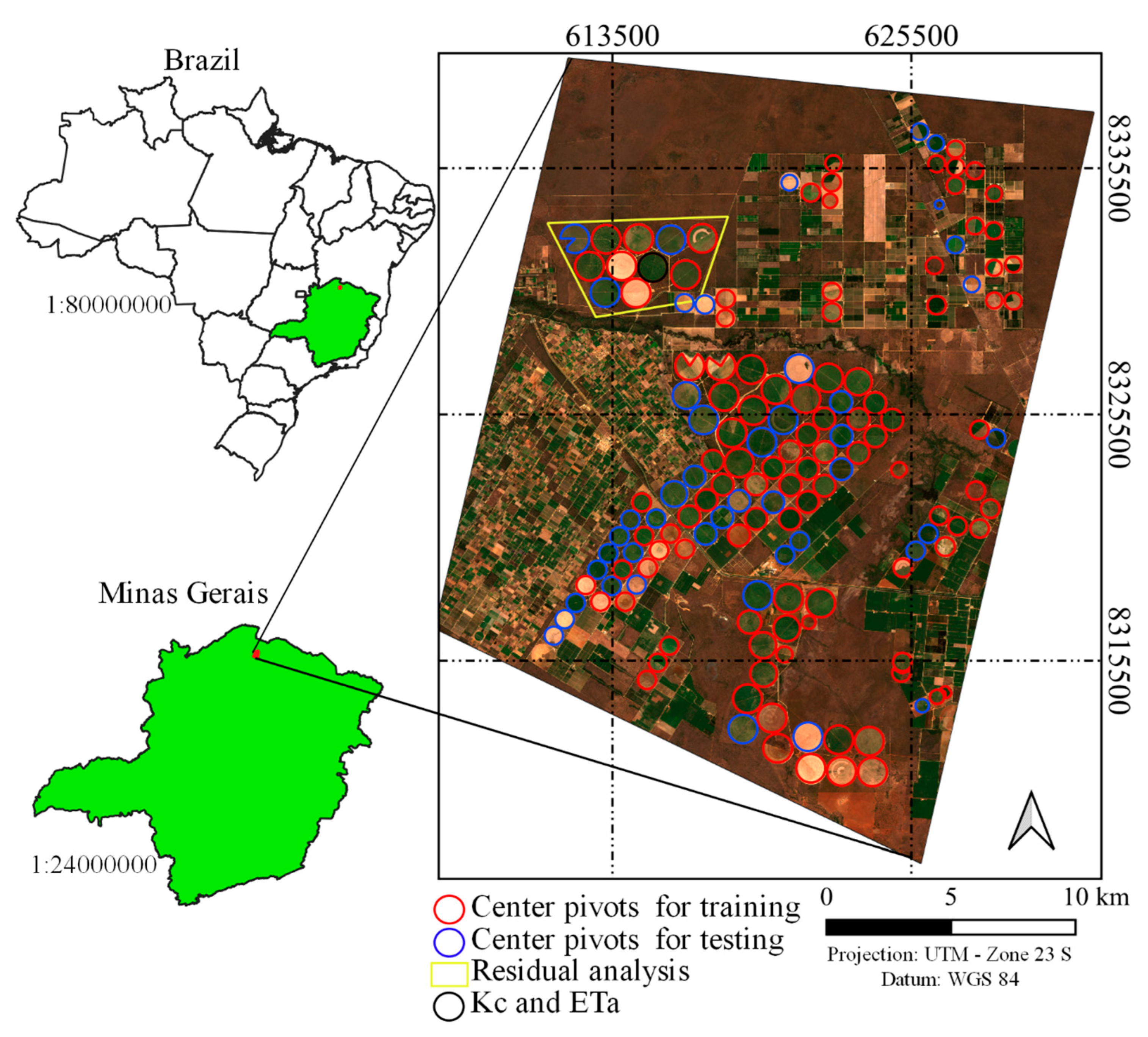
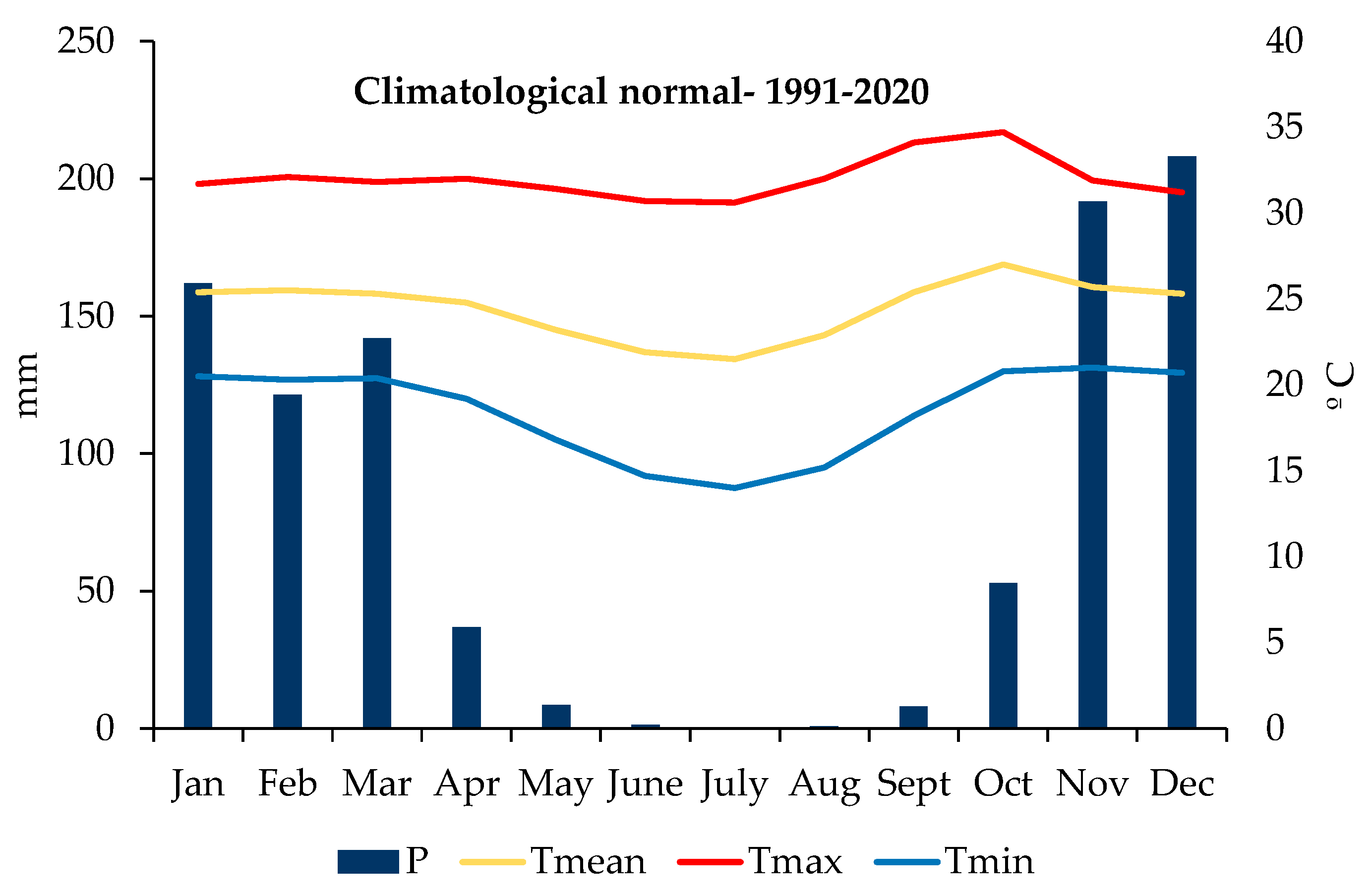
2.1. Study Area
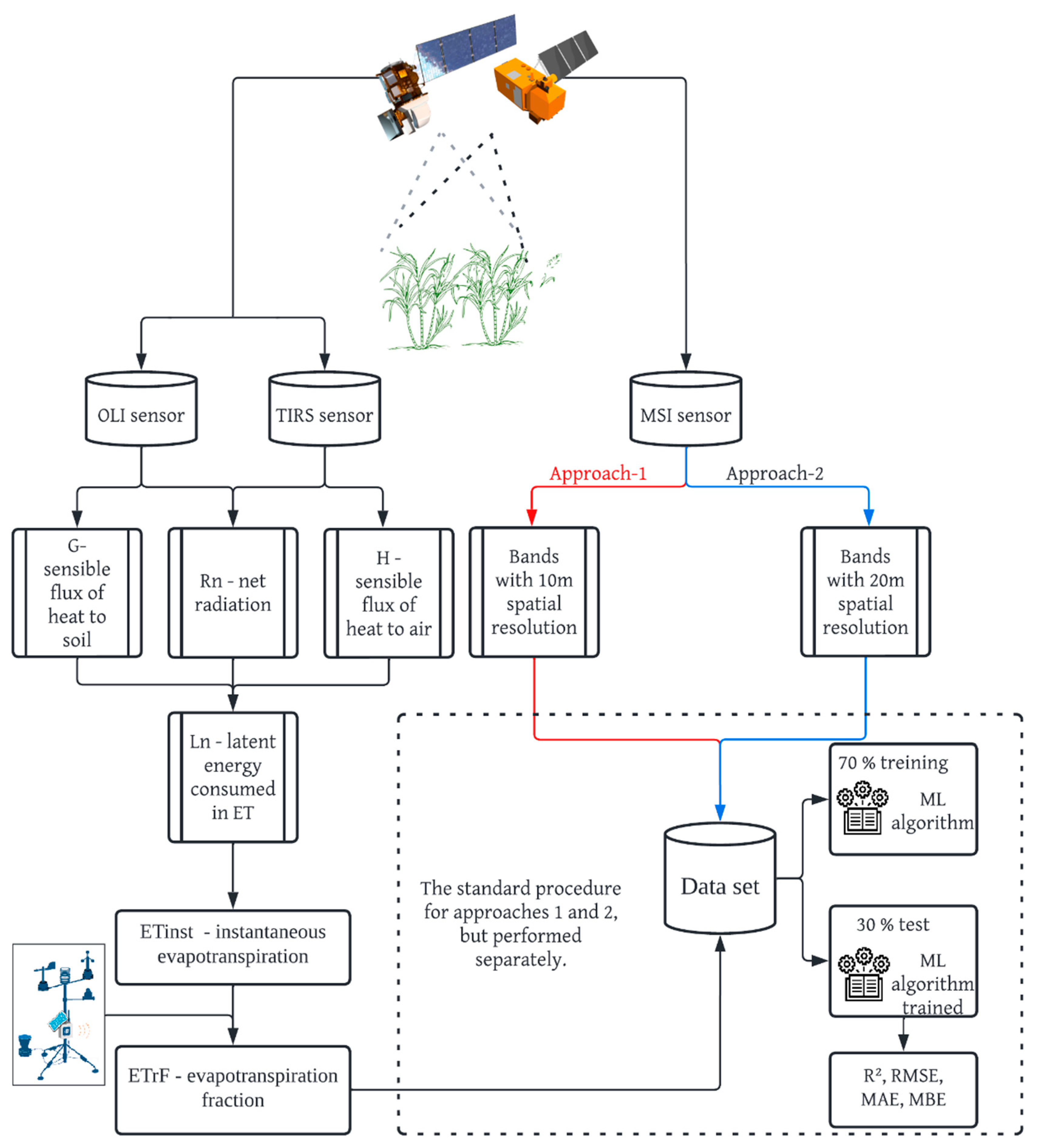
2.2. Landsat-8 and Sentinel-2 Data
2.3. Response Variable
2.4. Data Extraction for Training
2.5. Training and Statistical Evaluation of Models
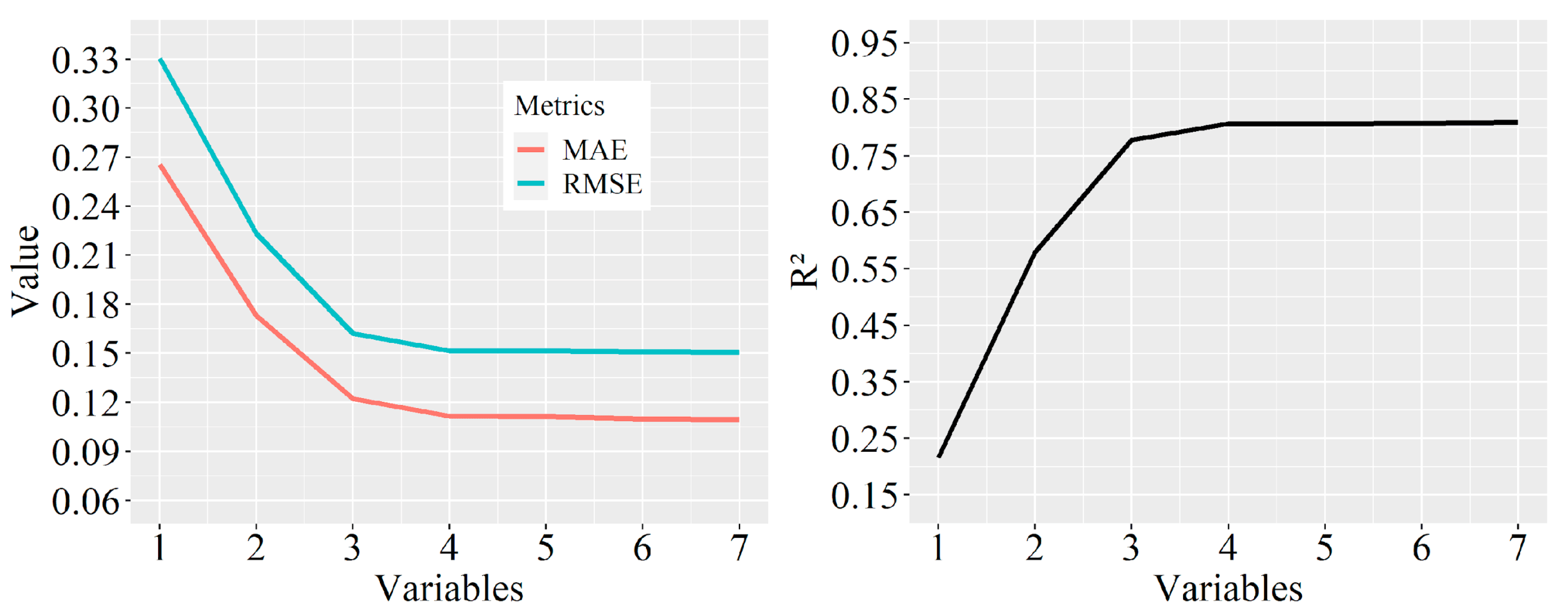
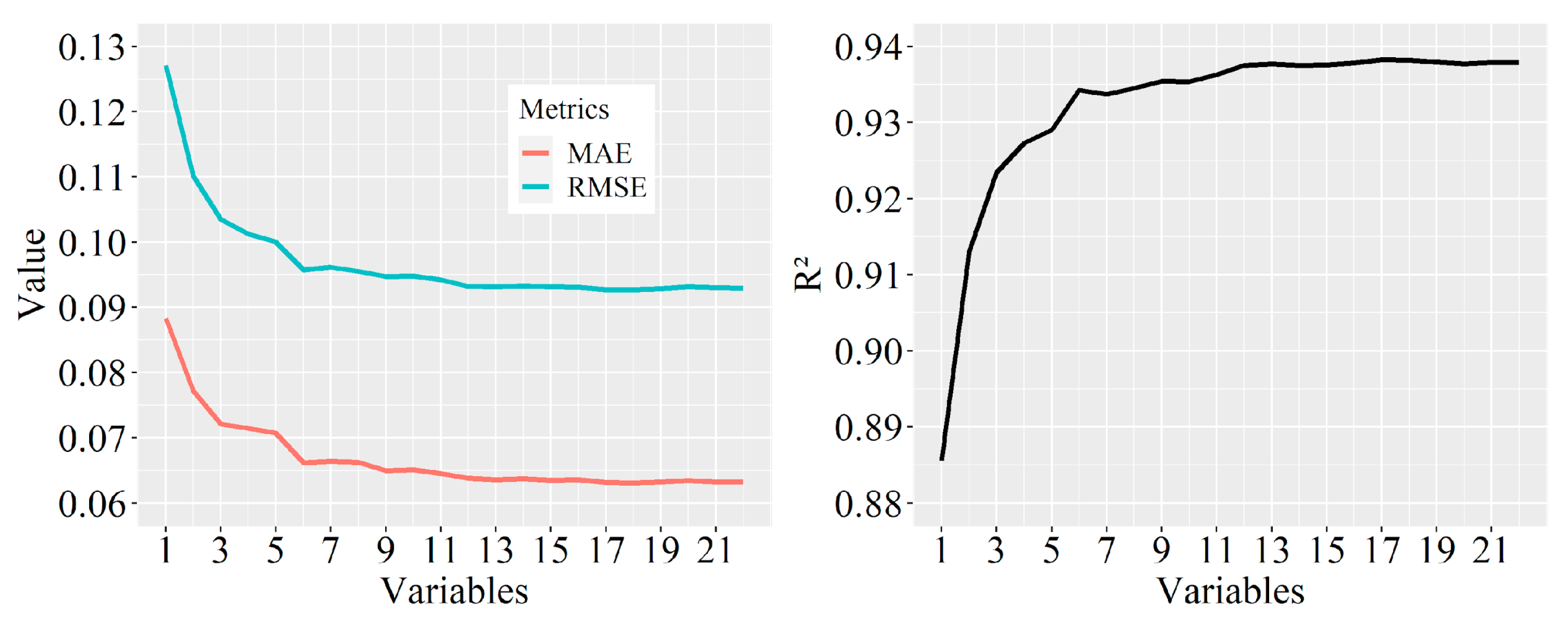
2.5.1. Production and Selection of Predictor Variables
2.5.2. Training and Test
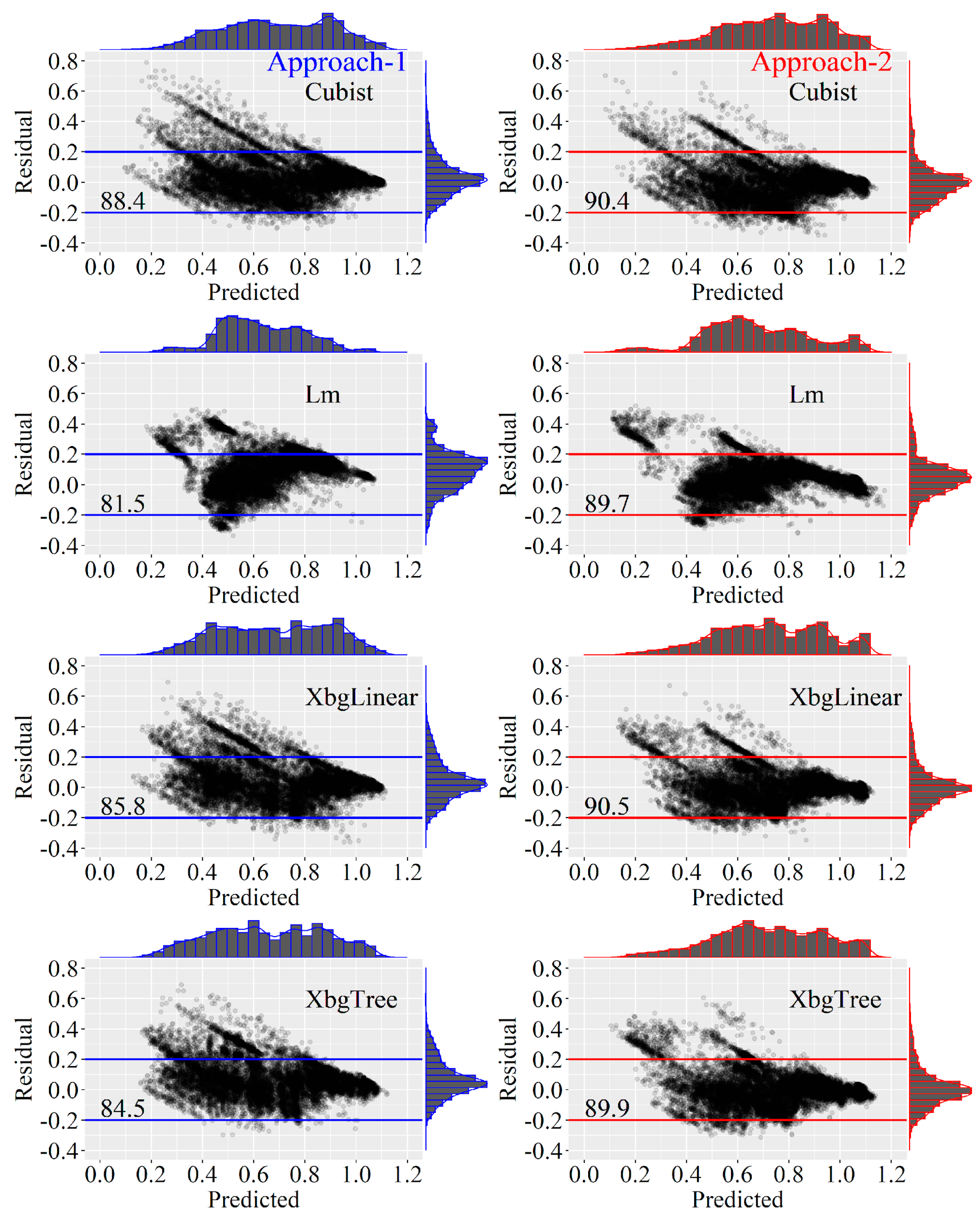
2.5.3. Residual Analysis
2.6. Application
3. Results
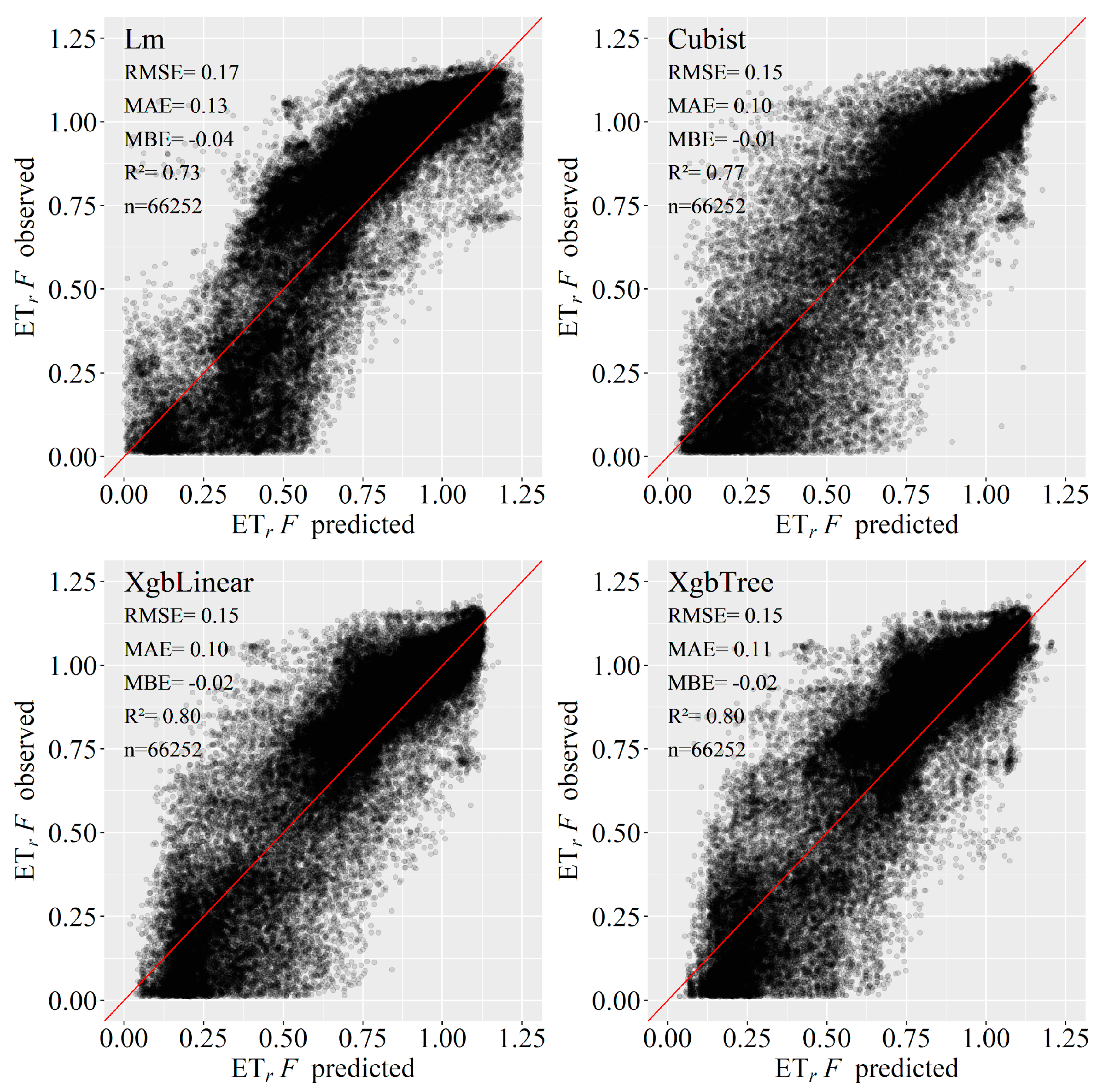
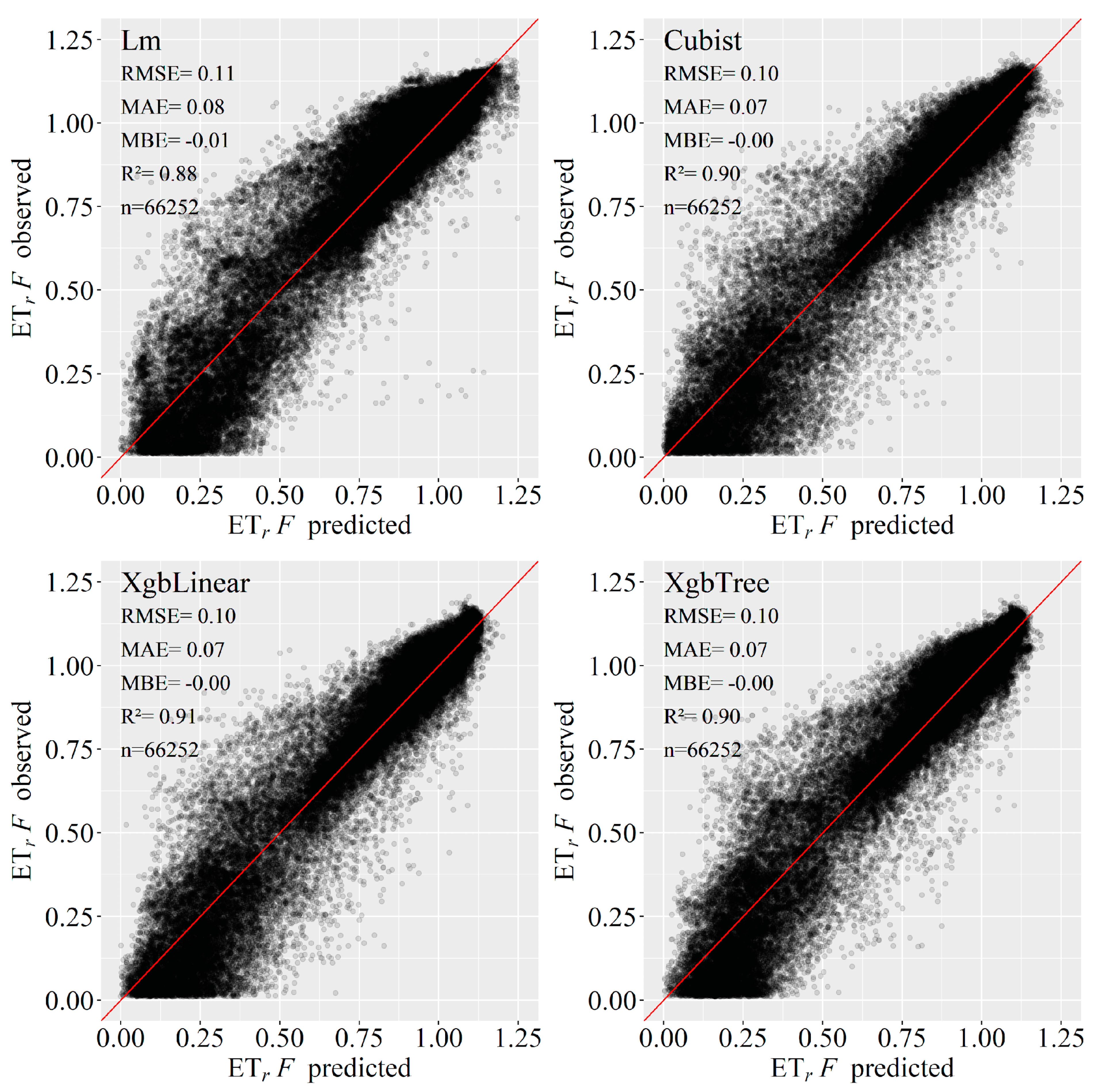
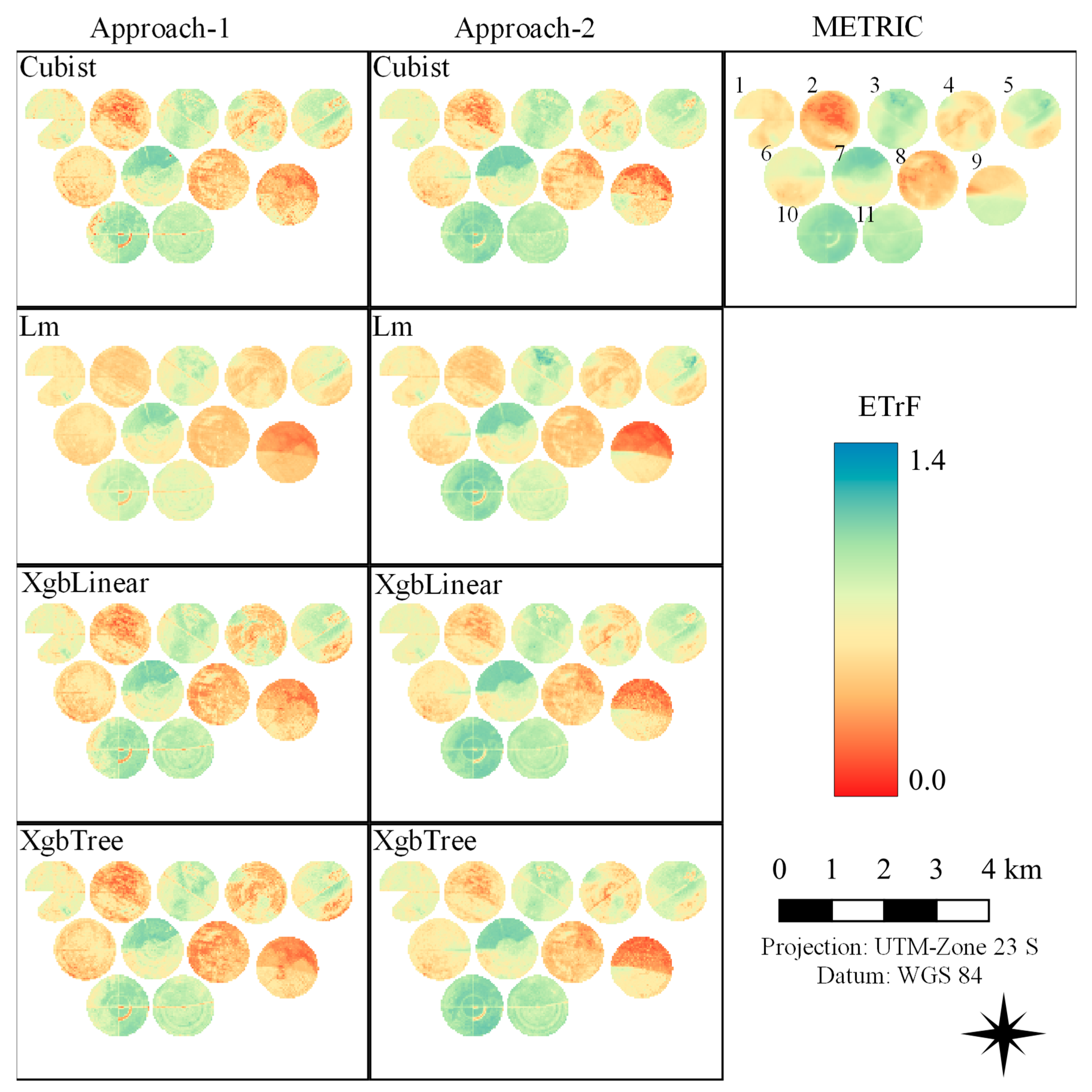
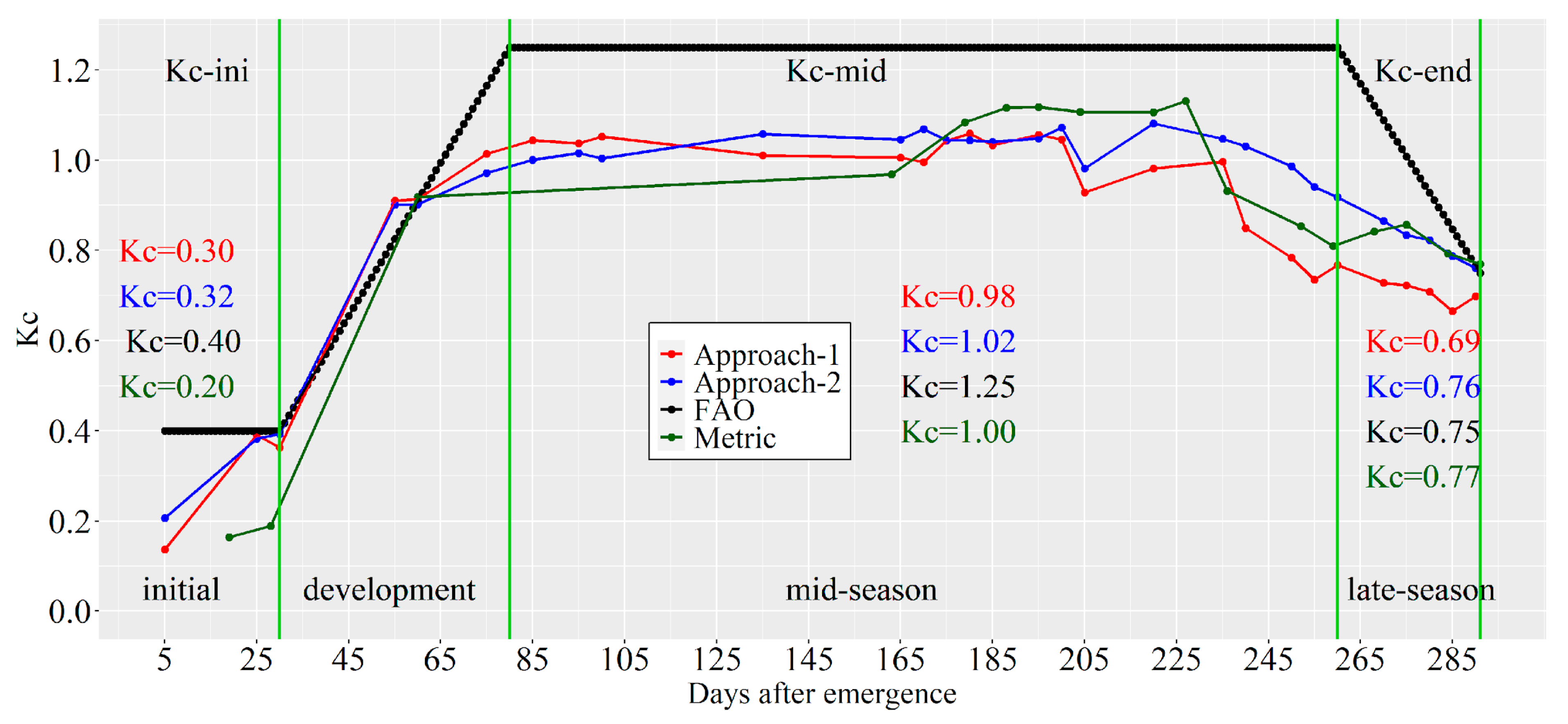
3.1. Models
3.2. Residual Analysis
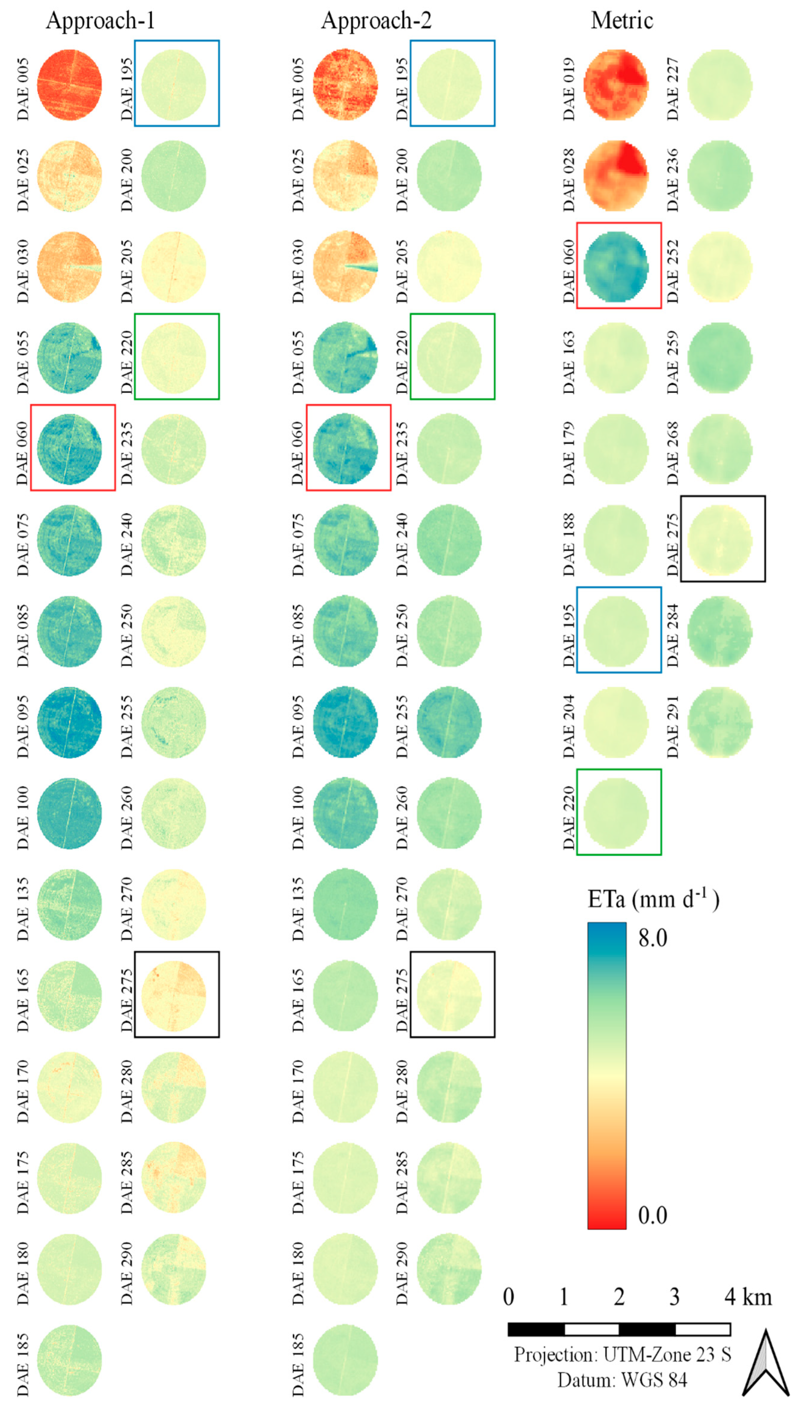
3.3. Models Application
4. Discussions
5. Conclusions
Supplementary Materials
Author Contributions
Funding
Data Availability Statement
Conflicts of Interest
Abbreviations
| ETa | Actual Evapotranspiration |
| ETints | Instantaneous Evapotranspiration |
| ETo | Reference Potential Evapotranspiration of the Grass |
| ETr | Reference Potential Evapotranspiration of the Afalfa |
| ETrF | Evapotranspiration Fraction |
| METRIC | Mapping Evapotranspiration at High Resolution with Internalized Calibration |
| ML | Machine Learning |
| MSI | MultiSpectral Instrument |
| OLI | Operational Land Imager |
| R2 | Coefficient of Determination |
| RMSE | Root Mean Squared Error |
| MAE | Mean Absolute Error |
| MBE | Mean Bias Error |
| SAFER | Simple Algorithm for Evapotranspiration Retrieving |
| SEBAL | Surface Energy Balance Algorithm for Land |
| TIRS | Thermal Infrared Sensor |
| P | Precipitation |
| Tmean | Mean Air Temperature |
| Tmax | Maximum Air Temperature |
| Tmin | Minimum Air Temperature |
| µm | Micrometer |
| m | Meter |
| Kc | Crop Coefficient |
| LE | Latent Energy |
| ρw | Density of Water |
| λ | Latent Heat of Vaporization |
| Ts | Surface Temperature |
| Rn | Net Radiation |
| G | Sensible Flux of Heat Transferred to the Ground |
| H | Sensible Flux of Heat Convected to Air |
| Rs↓ | Input of Shortwave Radiation |
| α | Surface Albedo |
| RL↓ | Input of Long Waves |
| RL↑ | Output of Long Waves |
| ԑ0 | Surface Thermal Emissivity |
| LAI | Leaf Area Index |
| ρair | Air Density |
| Cp | Specific Heat of Air at Constant Pressure |
| dT | Temperature Difference Between Two Heights |
| rah | Aerodynamic Drag |
| ρB | Reflectance of Blue |
| ρG | Reflectance of Green |
| ρR | Reflectance of Red |
| ρNIR | Reflectance of Near-Infrared |
| ρRe | Reflectance of Red Edge |
| ρSWIR | Reflectance of Shortwave Infrared |
| NRPB | Normalized Ratio Procedure Between Bands |
| LM | Linear Regression |
| Xgblinear | eXtreme Gradient Boosting-linear method |
| XgbTree | eXtreme Gradient Boosting-tree method |
| DAE | Days After Emergency |
| FAO | Food and Agriculture Organization |
References
- Allen, R.G.; Pereira, L.S.; Raes, D.; Smith, M. Table of Contents Originated by: Agriculture Crop Evapotranspiration—Guidelines for Computing Crop Water Requirements–FAO Irrigation and Drainage Paper 56, 9th ed.; Food and Agriculture Organization of the United Nations: Rome, Italy, 1998. [Google Scholar]
- Allen, R.; Irmak, A.; Trezza, R.; Hendrickx, J.M.H.; Bastiaanssen, W.; Kjaersgaard, J. Satellite-Based ET Estimation in Agriculture Using SEBAL and METRIC. Hydrol. Process. 2011, 25, 4011–4027. [Google Scholar] [CrossRef]
- Srivastava, A.; Sahoo, B.; Raghuwanshi, N.S.; Singh, R. Evaluation of Variable-Infiltration Capacity Model and MODIS-Terra Satellite-Derived Grid-Scale Evapotranspiration Estimates in a River Basin with Tropical Monsoon-Type Climatology. J. Irrig. Drain. Eng. 2017, 143, 1. [Google Scholar] [CrossRef]
- Bastiaanssen, W.G. SEBAL-Based Sensible and Latent Heat Fluxes in the Irrigated Gediz Basin, Turkey. J. Hydrol. 1999, 229, 87–100. [Google Scholar] [CrossRef]
- Teixeira, A.D.C.; Bastiaanssen, W.; Ahmad, M.-U.; Bos, M. Reviewing SEBAL Input Parameters for Assessing Evapotranspiration and Water Productivity for the Low-Middle São Francisco River Basin, Brazil. Part B: Application to the Regional Scale. Agric. For. Meteorol. 2009, 149, 477–490. [Google Scholar] [CrossRef]
- Bastiaanssen, W.G.M.; Pelgrum, H.; Wang, J.; Ma, Y.; Moreno, J.F.; Roerink, G.J.; van der Wal, T. A Remote Sensing Surface Energy Balance Algorithm for Land (SEBAL), Part 1: Formulation. J. Hydrol. 1998, 212–213, 213–229. [Google Scholar] [CrossRef]
- Allen, R.G.; Tasumi, M.; Trezza, R. Satellite-Based Energy Balance for Mapping Evapotranspiration with Internalized Calibration (METRIC)—Applications. J. Irrig. Drain. Eng. 2007, 133, 395–406. [Google Scholar] [CrossRef]
- Teixeira, A.H.d.C. Determining Regional Actual Evapotranspiration of Irrigated Crops and Natural Vegetation in the São Francisco River Basin (Brazil) Using Remote Sensing and Penman-Monteith Equation. Remote Sens. 2010, 2, 1287–1319. [Google Scholar] [CrossRef]
- Filgueiras, R.; Mantovani, E.C.; Dias, S.H.B.; Fernandes Filho, E.I.; da Cunha, F.F. Optimizing the Monitoring of Natural Phenomena Through the Coupling of Orbital Multi-Sensors. Geo UERJ. 2020, 37, 37832. [Google Scholar] [CrossRef]
- Berni, J.A.J.; Zarco-Tejada, P.J.; Sepulcre-Cantó, G.; Fereres, E.; Villalobos, F. Mapping Canopy Conductance and CWSI in Olive Orchards Using High Resolution Thermal Remote Sensing Imagery. Remote Sens. Environ. 2009, 113, 2380–2388. [Google Scholar] [CrossRef]
- Taiz, L.; Zeiger, E.; Moller, I.M.; Murphy, A. Plant Physiology & Development, 6th ed.; Sinauer Associates Incorporated: Sunderland, MA, USA, 2015; ISBN 9781605353531. [Google Scholar]
- Cervantes, J.; Garcia-Lamont, F.; Rodríguez-Mazahua, L.; Lopez, A. A Comprehensive Survey on Support Vector Machine Classification: Applications, Challenges and Trends. Neurocomputing 2020, 408, 189–215. [Google Scholar] [CrossRef]
- Adab, H.; Morbidelli, R.; Saltalippi, C.; Moradian, M.; Ghalhari, G.A.F. Machine Learning to Estimate Surface Soil Moisture from Remote Sensing Data. Water 2020, 12, 3223. [Google Scholar] [CrossRef]
- Filgueiras, R.; Mantovani, E.C.; Dias, S.H.B.; Fernandes Filho, E.I.; da Cunha, F.F.; Neale, C.M.U. New Approach to Determining the Surface Temperature without Thermal Band of Satellites. Eur. J. Agron. 2019, 106, 12–22. [Google Scholar] [CrossRef]
- Granata, F. Evapotranspiration Evaluation Models Based on Machine Learning Algorithms—A Comparative Study. Agric. Water Manag. 2019, 217, 303–315. [Google Scholar] [CrossRef]
- Tikhamarine, Y.; Malik, A.; Kumar, A.; Souag-Gamane, D.; Kisi, O. Estimation of Monthly Reference Evapotranspiration Using Novel Hybrid Machine Learning Approaches. Hydrol. Sci. J. 2019, 64, 1824–1842. [Google Scholar] [CrossRef]
- Virnodkar, S.S.; Pachghare, V.K.; Patil, V.C.; Jha, S.K. Remote Sensing and Machine Learning for Crop Water Stress Determination in Various Crops: A Critical Review. Precis. Agric. 2020, 21, 1121–1155. [Google Scholar] [CrossRef]
- Carter, C.; Liang, S. Evaluation of Ten Machine Learning Methods for Estimating Terrestrial Evapotranspiration from Remote Sensing. Int. J. Appl. Earth Obs. Geoinf. 2019, 78, 86–92. [Google Scholar] [CrossRef]
- Xu, T.; Guo, Z.; Xia, Y.; Ferreira, V.G.; Liu, S.; Wang, K.; Yao, Y.; Zhang, X.; Zhao, C. Evaluation of Twelve Evapotranspiration Products from Machine Learning, Remote Sensing and Land Surface Models over Conterminous United States. J. Hydrol. 2019, 578, 124105. [Google Scholar] [CrossRef]
- Chai, R.; Sun, S.; Chen, H.; Zhou, S. Changes in Reference Evapotranspiration over China during 1960–2012: Attributions and Relationships with Atmospheric Circulation. Hydrol. Process. 2018, 32, 3032–3048. [Google Scholar] [CrossRef]
- Kadkhodazadeh, M.; Anaraki, M.V.; Morshed-Bozorgdel, A.; Farzin, S. A New Methodology for Reference Evapotranspiration Prediction and Uncertainty Analysis under Climate Change Conditions Based on Machine Learning, Multi Criteria Decision Making and Monte Carlo Methods. Sustainability 2022, 14, 2601. [Google Scholar] [CrossRef]
- Raza, A.; Shoaib, M.; Faiz, M.A.; Baig, F.; Khan, M.M.; Ullah, M.K.; Zubair, M. Comparative Assessment of Reference Evapotranspiration Estimation Using Conventional Method and Machine Learning Algorithms in Four Climatic Regions. J. Pure Appl. Geophys. 2020, 177, 4479–4508. [Google Scholar] [CrossRef]
- Tang, D.; Feng, Y.; Gong, D.; Hao, W.; Cui, N. Evaluation of Artificial Intelligence Models for Actual Crop Evapotranspiration Modeling in Mulched and Non-Mulched Maize Croplands. Comput. Electron. Agric. 2018, 152, 375–384. [Google Scholar] [CrossRef]
- Alvares, C.A.; Stape, J.L.; Sentelhas, P.C.; De Moraes Gonçalves, J.L.; Sparovek, G. Köppen’s Climate Classification Map for Brazil. Meteorol. Zeitschrift 2013, 22, 711–728. [Google Scholar] [CrossRef]
- Tasumi, M. Progress in Operational Estimation of Regional Evapotranspiration Using Satellite Imagery; University of Idaho: Moscow, ID, USA, 2003. [Google Scholar]
- Olmedo, G.F.; Ortega-Farías, S.; Fonseca-Luengo, D.; de la Fuente-Sáiz, D.; Fuentes-peñailillo, F.; Munafó, M.V. Water: Actual Evapotranspiration with Energy Balance Models. Available online: https://cran.r-project.org/web/packages/water/water.pdf (accessed on 3 January 2021).
- R Core Team. R: A Language and Environment for Statistical Computing, version 3.3.1; R Foundation for Statistical Computing: Vienna, Austria, 2019. [Google Scholar]
- Hijmans, R.J.; van Etten, J.; Cheng, J.; Mattiuzzi, M.; Sumner, M.; Greenberg, J.A.; Lamigueiro, O.P.; Bevan, A.; Racine, E.B.; Shortridge, A.; et al. Raster: Geographic Data Analysis and Modeling. Available online: https://cran.r-project.org/web/packages/raster/index.html (accessed on 10 January 2021).
- Fernandes Filho, E.I. Labgeo: Collection of Functions to Fit Models with Emphasis in Land Use and Soil Mapping. Available online: https://rdrr.io/github/elpidiofilho/labgeo/ (accessed on 8 January 2021).
- Filgueiras, R.; Mantovani, E.C.; Althoff, D.; Fernandes Filho, E.I.; Cunha, F.F. da Crop NDVI Monitoring Based on Sentinel 1. Remote Sens. 2019, 11, 1441. [Google Scholar] [CrossRef]
- Kuhn, M.; Wing, J.; Weston, S.; Williams, A.; Keefer, C.; Engelhardt, A.; Cooper, T.; Mayer, Z.; Kenkel, B.; Team, R.C. Classification and Regression Training. Available online: https://cran.r-project.org/web/packages/caret/index.html (accessed on 8 January 2021).
- Allen, R.G.; Walter, I.A.; Elliott, R.; Howell, T.; Itenfisu, D.; Jensen, M. The ASCE Standardized Reference Evapotranspiration Equation; American Society of Civil Engineers: Reston, VA, USA, 2005. [Google Scholar]
- Ekstrøm, C.T. MESS: Miscellaneous Esoteric Statistical Scripts. Available online: https://cran.r-project.org/web/packages/MESS/index.html (accessed on 8 January 2021).
- Ke, Y.; Im, J.; Park, S.; Gong, H. Spatiotemporal Downscaling Approaches for Monitoring 8-Day 30 m Actual Evapotranspiration. ISPRS J. Photogramm. Remote Sens. 2017, 126, 79–93. [Google Scholar] [CrossRef]
- Dingre, S.K.; Gorantiwar, S.D. Determination of the Water Requirement and Crop Coefficient Values of Sugarcane by Field Water Balance Method in Semiarid Region. Agric. Water Manag. 2020, 232, 106042. [Google Scholar] [CrossRef]
- da Silva, T.G.F.; de Moura, M.S.B.; Zolnier, S.; Soares, J.M.; Vieira, V.J.d.S.; Júnior, W.G.F. Water Requirement and Crop Coefficient of Irrigated Sugarcane in a Semi-Arid Region. Rev. Bras. Eng. Agric. Ambient. 2012, 16, 64–71. [Google Scholar] [CrossRef]
- Saleem, A.; Awange, J.L. Coastline Shift Analysis in Data Deficient Regions: Exploiting the High Spatio-Temporal Resolution Sentinel-2 Products. CATENA 2019, 179, 6–19. [Google Scholar] [CrossRef]
- de Silva, V.D.P.; Garcêz, S.L.A.; Silva, B.B.D.; De Albuquerque, M.F.; Almeida, R.S.R. Métodos de Estimativa Da Evapotranspiração Da Cultura Da Cana-de-Açúcar Em Condições de Sequeiro. Rev. Bras. Eng. Agríc. Ambient 2015, 19, 411–417. [Google Scholar] [CrossRef]
- Li, D.; Li, W.; Zhang, H.; Zhang, X.; Zhuang, J.; Liu, Y.; Hu, C.; Lei, B. Far-Red Carbon Dots as Efficient Light-Harvesting Agents for Enhanced Photosynthesis. ACS Appl. Mater. Interfaces 2020, 12, 21009–21019. [Google Scholar] [CrossRef]
- Wang, Y.; Xie, Z.; Wang, X.; Peng, X.; Zheng, J. Fluorescent Carbon-Dots Enhance Light Harvesting and Photosynthesis by Overexpressing PsbP and PsiK Genes. J. Nanobiotechnol. 2021, 19, 260. [Google Scholar] [CrossRef]
- Ponzoni, F.J.; Shimabukuro, Y.E.; Kuplich, T.M. Sensoriamento Remoto Da Vegetação, 2nd ed.; Oficina de Textos: São Paulo, Brazil, 2012; ISBN 978-85-7975-053-3. [Google Scholar]
- dos Santos, N.V.; Demattê, J.A.M.; Silvero, N.E.Q. Improving the Monitoring of Sugarcane Residues in a Tropical Environment Based on Laboratory and Sentinel-2 Data. Int. J. Remote Sens. 2020, 42, 1768–1784. [Google Scholar] [CrossRef]
- Chandel, N.S.; Rajwade, Y.A.; Golhani, K.; Tiwari, P.S.; Dubey, K.; Jat, D. Canopy Spectral Reflectance for Crop Water Stress Assessment in Wheat (Triticum aestivum, L.). Irrig. Drain. 2020, 70, 321–331. [Google Scholar] [CrossRef]
- Chen, H.; Wang, P.; Li, J.; Zhang, J.; Zhong, L. Canopy Spectral Reflectance Feature and Leaf Water Potential of Sugarcane Inversion. Phys. Procedia 2012, 25, 595–600. [Google Scholar] [CrossRef][Green Version]
- Gates, D.M.; Keegan, H.J.; Schleter, J.C.; Weidner, V.R. Spectral Properties of Plants. Appl. Opt. 1965, 4, 11. [Google Scholar] [CrossRef]
- Muller, S.J.; Sithole, P.; Singels, A.; Van Niekerk, A. Assessing the Fidelity of Landsat-Based FAPAR Models in Two Diverse Sugarcane Growing Regions. Comput. Electron. Agric. 2020, 170, 105248. [Google Scholar] [CrossRef]
- Zhang, F.; Zhou, G. Estimation of Vegetation Water Content Using Hyperspectral Vegetation Indices: A Comparison of Crop Water Indicators in Response to Water Stress Treatments for Summer Maize. BMC Ecol. 2019, 19, 18. [Google Scholar] [CrossRef] [PubMed]
- Jamshidi, S.; Zand-Parsa, S.; Pakparvar, M.; Niyogi, D. Evaluation of Evapotranspiration over a Semiarid Region Using Multiresolution Data Sources. J. Hydrometeorol. 2019, 20, 947–964. [Google Scholar] [CrossRef]
- Nisa, Z.; Khan, M.S.; Govind, A.; Marchetti, M.; Lasserre, B.; Magliulo, E.; Manco, A. Evaluation of SEBS, METRIC-EEFlux, and QWaterModel Actual Evapotranspiration for a Mediterranean Cropping System in Southern Italy. Agronomy 2021, 11, 345. [Google Scholar] [CrossRef]
- Ortega-Salazar, S.; Ortega-Farías, S.; Kilic, A.; Allen, R. Performance of the METRIC Model for Mapping Energy Balance Components and Actual Evapotranspiration over a Superintensive Drip-Irrigated Olive Orchard. Agric. Water Manag. 2021, 251, 106861. [Google Scholar] [CrossRef]


| Spectral Band | Wavelength (μm) | Spatial Resolution (m) | |
|---|---|---|---|
| OLI | |||
| B1 | Coastal aerosol (Ca) | 0.43–0.45 | 30 |
| B2 | Blue (B) | 0.45–0.51 | |
| B3 | Green (G) | 0.53–0.59 | |
| B4 | Red (R) | 0.64–0.67 | |
| B5 | Near-infrared (NIR) | 0.85–0.88 | |
| B6 | Shortwave infrared 1 (SWIR1) | 1.57–1.65 | |
| B7 | Shortwave infrared 2 (SWIR2) | 2.11–2.29 | |
| B8 | Panchromatic (PCh) | 0.50–0.68 | |
| B9 | Cirrus (C) | 1.36–1.38 | |
| TIRS | |||
| B10 | Thermal infrared 1 (TIRS1) | 10.60–11.19 | 100 * |
| B11 | Thermal infrared 2 (TIRS2) | 11.50–12.51 | |
| Spectral Band | Wavelength (μm) | Spatial Resolution (m) | |
|---|---|---|---|
| MSI | |||
| B2 | Blue (B) | 0.459–0.525 | 10 |
| B3 | Green (G) | 0.542–0.578 | |
| B4 | Red (R) | 0.650–0.680 | |
| B8 | Near-infrared (NIR) | 0.781–0.887 | |
| B5 | red edge 1 (Re1) | 0.697–0.712 | 20 |
| B6 | red edge 2 (Re2) | 0.733–0.748 | |
| B7 | red edge 3 (Re2) | 0.773–0.793 | |
| B8A | Near-infrared narrow (NIRn) | 0.856–0.876 | |
| B11 | Shortwave infrared 1 (SWIR1) | 1.569–1.660 | |
| B12 | Shortwave infrared 2 (SWIR2) | 2.115–2.290 | |
| B1 | Coastal aerosol | 0.433–0.453 | 60 |
| B9 | Water vapor | 0.935–0.955 | |
| B10 | Cirrus | 1.359–1.390 | |
| Date (mm/dd/aaaa) | Landsat-8 | Sentinel-2 | ||
|---|---|---|---|---|
| Time (hh:mm:ss) | Path/Row | Time (hh:mm:ss) | Tile Number | |
| Training and Test | ||||
| 07/06/2018 | 09:55:17.157 | 218/71 | 10:12:41.024 | T23LPD |
| 05/22/2019 | 09:55:49.714 | 218/71 | 10:12:51.024 | T23LPD |
| 10/04/2019 | 10:02:19.874 | 219/70 | 10:12:49.024 | T23LPD |
| 10/29/2019 | 09:56:34.656 | 218/71 | 10:12:49.024 | T23LPD |
| 01/17/2020 | 09:56:20.969 | 218/71 | 10:12:41.024 | T23LPD |
| 05/31/2020 | 10:01:27.427 | 219/70 | 10:12:49.024 | T23LPD |
| 08/19/2020 | 10:02:00.995 | 219/70 | 10:12:49.024 | T23LPD |
| Residual analysis | ||||
| 12/02/2020 | 09:56:32.117 | 218/71 | 10:12:41.024 | T23LPD |
| N° | Approach 1 | Approach 2 |
|---|---|---|
| 1 | B2 | B6 |
| 2 | B4 | B8 |
| 3 | B8 | B12 |
| 4 | (B2 − B3)/(B2 + B3) | (B2 − B3)/(B2 + B3) |
| 5 | (B2 − B4)/(B2 + B4) | (B2 − B4)/(B2 + B4) |
| 6 | - | (B2 − B5)/(B2 + B5) |
| 7 | - | (B2 − B12)/(B2 + B12) |
| 8 | - | (B5 − B11)/(B5 + B11) |
| 9 | - | (B5 − B12)/(B5 + B12) |
| 10 | - | (B6 − B8)/(B6 + B8) |
| 11 | - | (B8 − B12)/(B8 + B12) |
| 12 | - | (B11 − B12)/(B11 + B12) |
| DAE | Approach 1 | Approach 2 | METRIC | Difference (%) | |
|---|---|---|---|---|---|
| (mm) | (mm) | (mm) | Approach 1 | Approach 2 | |
| 060 | 6.71 ± 0.44 | 6.63 ± 0.36 | 6.75 ± 0.25 | 0.59 | 1.77 |
| 195 | 4.52 ± 0.22 | 4.48 ± 0.09 | 4.78 ± 0.06 | 5.44 | 6.28 |
| 220 | 4.25 ± 0.21 | 4.68 ± 0.11 | 4.79 ± 0.08 | 11.27 | 2.30 |
| 275 | 3.75 ± 0.36 | 4.32 ± 0.20 | 4.44 ± 0.17 | 16.54 | 2.77 |
| ET-Total | 1417.77 | 1474.26 | 1544.11 | 8.18 | 4.52 |
Publisher’s Note: MDPI stays neutral with regard to jurisdictional claims in published maps and institutional affiliations. |
© 2022 by the authors. Licensee MDPI, Basel, Switzerland. This article is an open access article distributed under the terms and conditions of the Creative Commons Attribution (CC BY) license (https://creativecommons.org/licenses/by/4.0/).
Share and Cite
dos Santos, R.A.; Mantovani, E.C.; Fernandes-Filho, E.I.; Filgueiras, R.; Lourenço, R.D.S.; Bufon, V.B.; Neale, C.M.U. Modeling Actual Evapotranspiration with MSI-Sentinel Images and Machine Learning Algorithms. Atmosphere 2022, 13, 1518. https://doi.org/10.3390/atmos13091518
dos Santos RA, Mantovani EC, Fernandes-Filho EI, Filgueiras R, Lourenço RDS, Bufon VB, Neale CMU. Modeling Actual Evapotranspiration with MSI-Sentinel Images and Machine Learning Algorithms. Atmosphere. 2022; 13(9):1518. https://doi.org/10.3390/atmos13091518
Chicago/Turabian Styledos Santos, Robson Argolo, Everardo Chartuni Mantovani, Elpídio Inácio Fernandes-Filho, Roberto Filgueiras, Rodrigo Dal Sasso Lourenço, Vinícius Bof Bufon, and Christopher M. U. Neale. 2022. "Modeling Actual Evapotranspiration with MSI-Sentinel Images and Machine Learning Algorithms" Atmosphere 13, no. 9: 1518. https://doi.org/10.3390/atmos13091518
APA Styledos Santos, R. A., Mantovani, E. C., Fernandes-Filho, E. I., Filgueiras, R., Lourenço, R. D. S., Bufon, V. B., & Neale, C. M. U. (2022). Modeling Actual Evapotranspiration with MSI-Sentinel Images and Machine Learning Algorithms. Atmosphere, 13(9), 1518. https://doi.org/10.3390/atmos13091518