
Effects of Urban Landscapes on Pollutant Concentrations in Chengdu Plain Urban Agglomeration


Abstract
:1. Introduction
2. Data and Methods
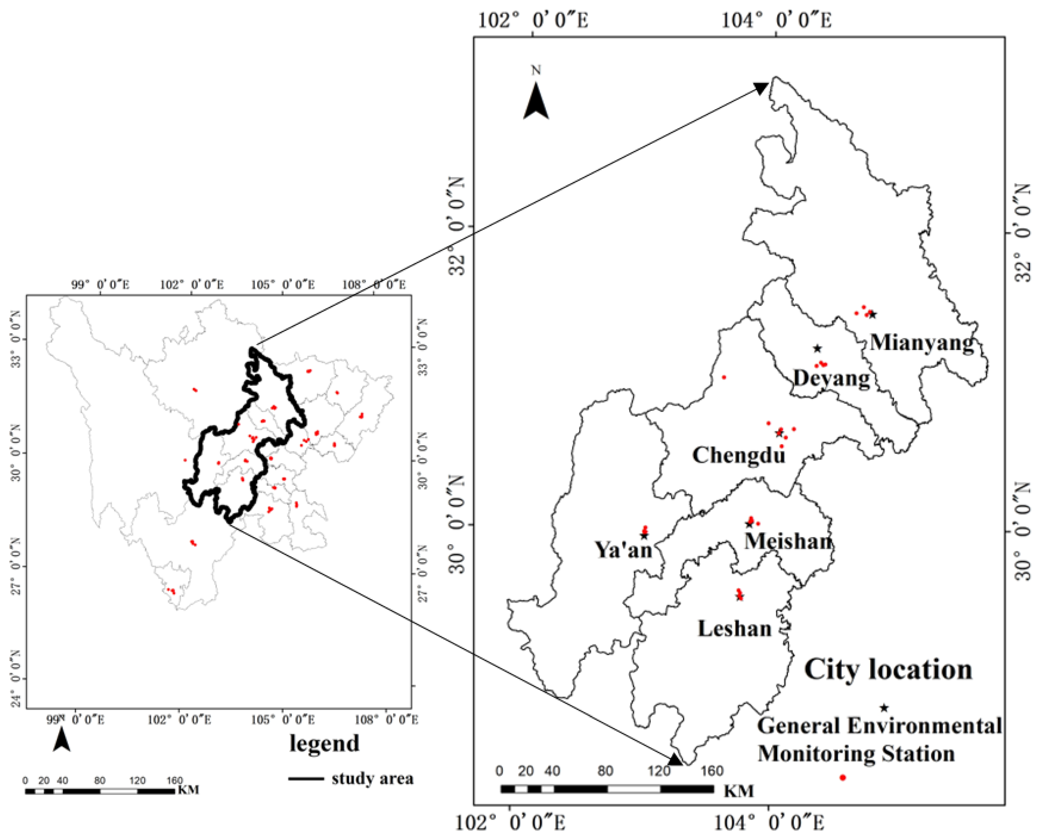
2.1. Study Area
2.2. Data Sources
2.3. Research Methods
3. Results
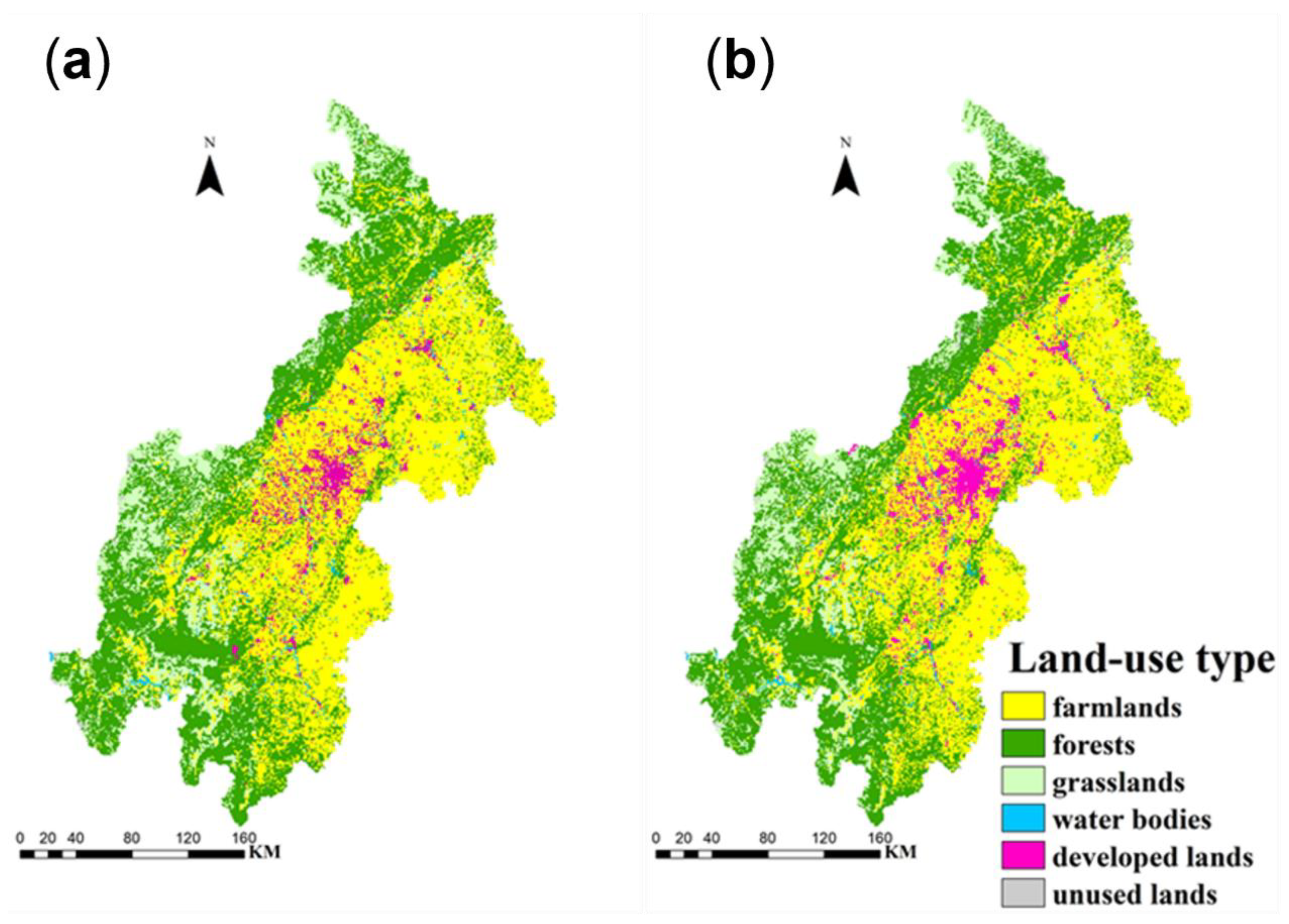
3.1. LP Analysis
3.1.1. LP Analysis at the Patch-Type Level
3.1.2. LP at the Landscape Level
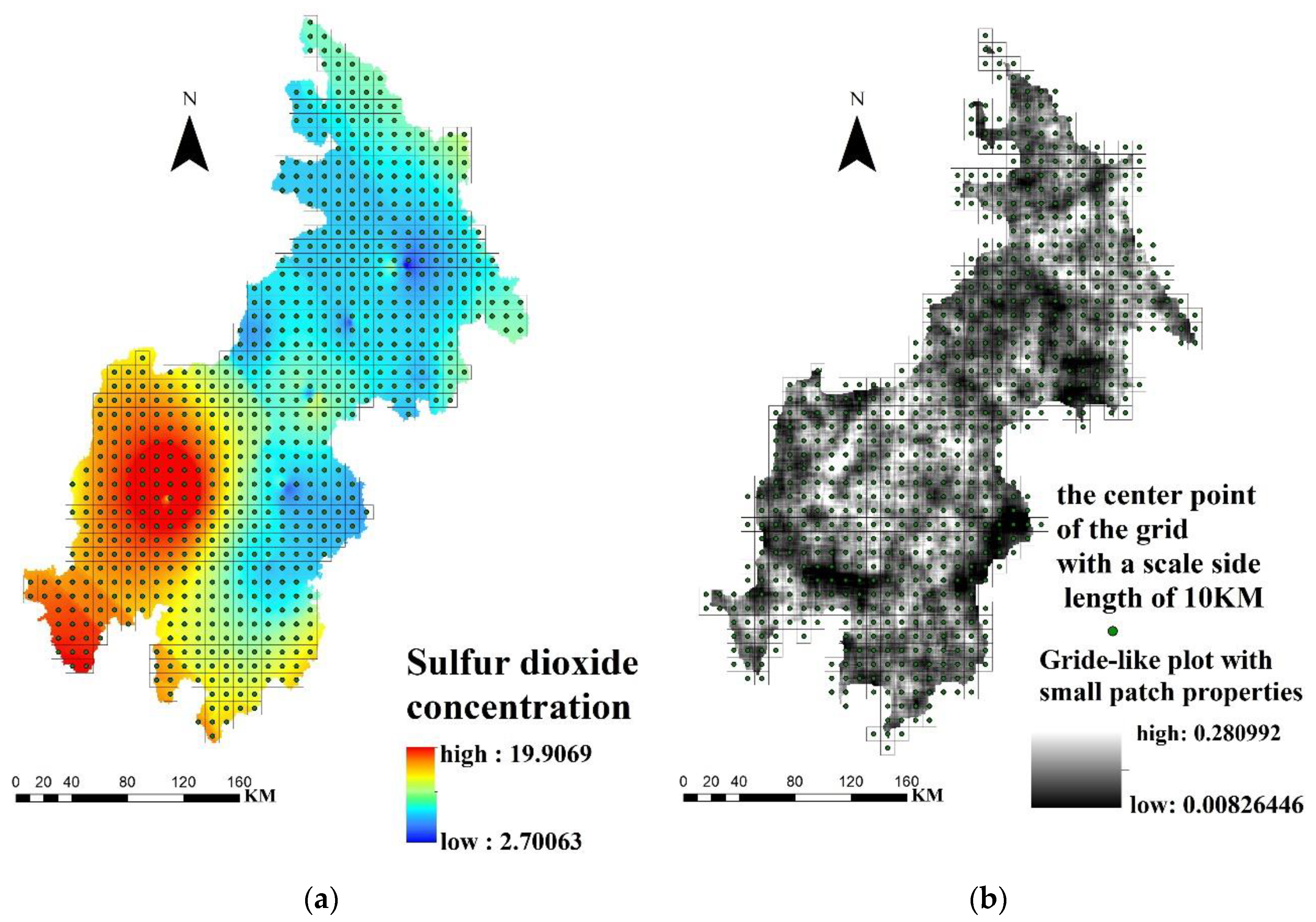
3.2. Spatial Distribution Patterns of the Concentrations of the Pollutants
3.3. Multiscale Coupling Relationships between the LP and the Concentrations of the Pollutants
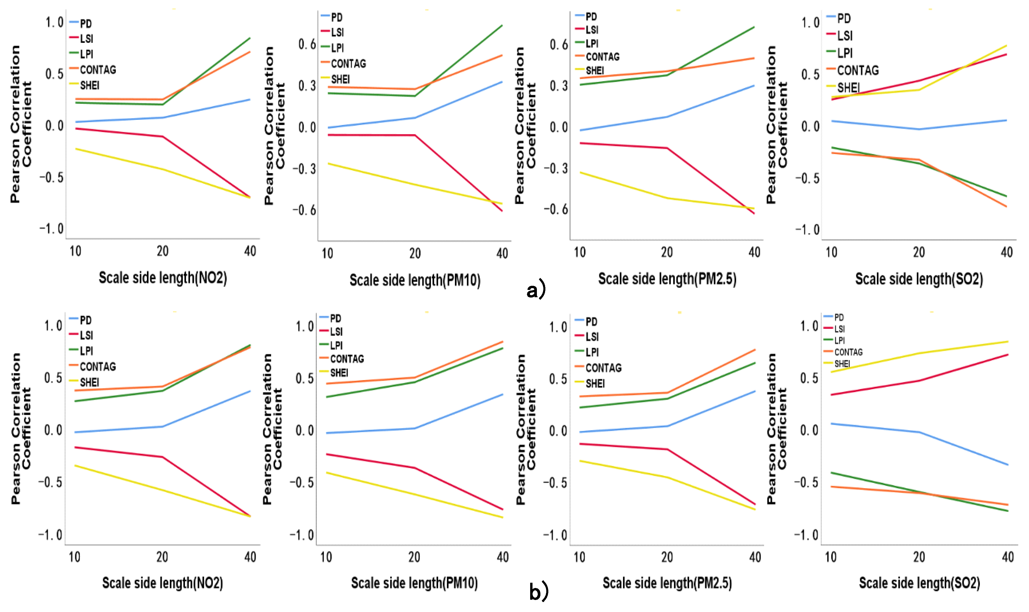
3.3.1. Coupling Relationships between the Concentrations of the Four Pollutants and the Overall LP in Different Years and at Different Scales
3.3.2. Coupling Relationships between the Concentrations of the Four Pollutants and the Six Landscape Types
4. Discussion
Author Contributions
Funding
Institutional Review Board Statement
Informed Consent Statement
Data Availability Statement
Acknowledgments
Conflicts of Interest
References
- Liu, H.J. Evaluation of the types of urban landscapes and their environmental ecological efficiency. J. South China Norm. Univ. (Nat. Sci. Ed.) 2003, 3, 126–130. [Google Scholar] [CrossRef]
- An, Z.; Huang, R.J.; Zhang, R.; Tie, X.; Li, G.; Cao, J.; Zhou, W.; Shi, Z.; Han, Y.; Gu, Z.; et al. Severe haze in northern China: A synergy of anthropogenic emissions and atmospheric processes. Proc. Natl. Acad. Sci. USA 2019, 116, 8657–8666. [Google Scholar] [CrossRef] [PubMed]
- Peng, C.L.; Wen, D.Z.; Sun, Z.J.; Lin, G.Y.; Lin, Z.F. Response of urban greenery to air pollution. J. Trop. Subtrop. Botany 2002, 10, 321–327. [Google Scholar] [CrossRef]
- Cao, Y.; Wang, C.X.; Liu, W.H.; Zhao, X.L. Analysis of air pollution characteristics of Chengdu from 2014 to 2017. Plateau Mt. Meteorol. Stud. 2019, 39, 48–54. [Google Scholar] [CrossRef]
- Mao, H.M.; Zhang, K.S.; Di, B.F.; Yang, J.J.; Ma, S. Spatial-temporal allocation of high resolution for air pollutant emission inventories in Chengdu. Acta Sci. Circumstantiae 2017, 37, 23–33. [Google Scholar] [CrossRef]
- Wu, S.P. Seasonal variation of air pollutants in Chengdu. Technol. Wind 2017, 23, 2. [Google Scholar] [CrossRef]
- Chen, F.B. Landscape Pattern Analysis and Optimization of Green Space System in Downtown Chengdu. Master’s Thesis, Southwest University, Chongqing, China, 2008. Available online: https://kns.cnki.net/kcms/detail/detail.aspx?dbcode=CMFD&dbname=CMFD2008&filename=2008093025.nh&uniplatform=NZKPT&v=6vcOXjUN0HVCcV_WxH39RGPB0RITI_Pz2LlnHv85IQXk5CDBQaGQKH3weoZ6wf1o (accessed on 13 March 2021).
- Wang, J.; Hou, L.G.; He, X.Q. Land use change and its ecological and environmental effects in the Chengdu Plain Urban Agglomeration from 2000 to 2019. Bull. Soil Water Conserv. 2022, 42, 360–368. [Google Scholar] [CrossRef]
- Deng, J. Research on landscape pattern optimization of urban green space based on air pollution control: A case study of yongzhou city. Xiandai Hortic. 2019, 42, 8–10. [Google Scholar] [CrossRef]
- Guan, J. Study on the Influence of Shijiazhuang Urban Landscape Pattern on Haze Effect. Master’s Thesis, Nanjing Normal University, Nanjing, China, 2015. Available online: https://kns.cnki.net/kcms/detail/detail.aspx?dbcode=CMFD&dbname=CMFD201601&filename=1015430413.nh&uniplatform=NZKPT&v=BLGIjRr1RVcC8E3rMsAe1kgNNWTW-FrVQFs09GaGp3Dqx9W-6al81Tvl7Hejolq6 (accessed on 13 March 2021).
- Qiu, Y.S. To Study the Correlation between the Distribution of Air Pollutants and the Landscape Pattern of Green Space in Wuhan. Master’s Thesis, Huazhong Agricultural University, Wuhan, China, 2018. Available online: https://kns.cnki.net/kcms/detail/detail.aspx?dbcode=CMFD&dbname=CMFD201801&filename=1017194842.nh&uniplatform=NZKPT&v=o6Z8Vv7TTjgWv3D-WWnTj8a6VqTNL0gzWnaYTzvQZzSf3GKppqbcWWYqo9ikSNGf (accessed on 15 March 2021).
- Min, S. Effect of Urban Landscape Pattern on the Variation of PM2.5 Concentration in Space-Time. Master’s Thesis, Zhejiang University of Agriculture and Forestry, Hangzhou, China, 2017. Available online: https://kns.cnki.net/kcms/detail/detail.aspx?dbcode=CMFD&dbname=CMFD201801&filename=1017273802.nh&uniplatform=NZKPT&v=5GJCiHrTLlwm7HuY_uRnpWKR2y_Dw4FqJPcf2FheLcBWwyfHdqli-PkmJTnGeoWK (accessed on 15 March 2021).
- Xie, W.D.; Wu, J.S. Effects of land use and landscape patterns on PM2.5 concentration: A case study of Shenzhen City. J. Peking Univ. Nat. Sci. Ed. 2017, 53, 19–25. [Google Scholar] [CrossRef]
- Han, X.; Huang, X.Y.; Ma, Y.X. Analysis of Urban Forest Landscape in Nanchang Based on GIS Technology. For. Inventory Plan. 2019, 44, 4. [Google Scholar] [CrossRef]
- Zhou, Y.; Shi, T.M.; Hu, Y.M.; Liu, M. Research on Green Landscape Optimization Based on Urban Climate Environment. City Plan Rev. 2014, 38, 7. [Google Scholar] [CrossRef]
- Liu, Q.; Wang, N.; Yang, L.W.; Qin, Y.W.; Zhao, J.; Zhang, X.; Zhang, P. Study on the Relation between Urban Landscape Pattern and Atmospheric Particle matter Pollution. Environ. Prot. Circ. Econ. 2020, 40, 58–63. [Google Scholar] [CrossRef]
- Zhang, S.Y. Analysis of Landscape Ecological Pattern and Process of Jiang’an Campus of Sichuan University. Sichuan Archit. 2019, 39, 15–16. [Google Scholar] [CrossRef]
- Wang, J. A Study on the Landscape Pattern of Small Towns in Nanning City. Master’s Thesis, Guangxi Normal University, Nanning, China, 2013. Available online: https://kns.cnki.net/kcms/detail/detail.aspx?dbcode=CMFD&dbname=CMFD201401&filename=1013315498.nh&uniplatform=NZKPT&v=9GQ_UHKgOWf-rpOnvN89sjFtI783iecEBOzC2MzeHxjKr1LC-YLWjJ3JvDyuz6L7 (accessed on 15 March 2021).
- Ma, X.P.; Han, S.S.; Wang, L.; Wang, J.X.; He, W. Characteristics and vulnerability differences in the North-South River Basin of Qinling Mountains. Hubei Agric. Sci. 2020, 59, 151–159. [Google Scholar] [CrossRef]
- Gao, L.; Tang, l.; Hou, H.L.; Wang, Y.; Mai, Y.Q.; He, W.B.; Wang, W.M.; Su, H.B. Spatiotemporal distribution of air pollution in Shenzhen and its relationship with landscape pattern. Acta Ecol. Sinica 2021, 41, 8758–8770. [Google Scholar] [CrossRef]
- Li, D.K.; Liu, M.; Li, L.C.; Hu, Y.M.; Wang, C.; Liu, C. The relationship between urban atmospheric environment and 2 D and 3 D landscape pattern of surrounding areas. Chin. J. Appl. Ecol. 2021, 32, 10. [Google Scholar] [CrossRef]
- Yang, J.; Mcbride, J.; Zhou, J.; Sun, Z.J.U.F.; Greening, U. The urban forest in Beijing and its role in air pollution reduction. Urban For. Urban Green. 2005, 3, 65–78. [Google Scholar] [CrossRef]
- Sun, M.; Chen, J.; Lin, X.T.; Yang, S. The Effect of Urban Landscape Pattern on PM2.5 Pollution. J. Zhejiang A F Univ. 2018, 35, 135–144. [Google Scholar] [CrossRef]
- Tao, Y.; Li, F.; Wang, R.S.; Zhao, D. Research Progress of Urban Green Spatial Pattern. Acta Ecol. Sinica 2013, 33, 2330–2342. [Google Scholar] [CrossRef]
- Wen, X.; Zhang, P.; Liu, D.J. Spatiotemporal Variations and Influencing Factors Analysis of PM_(2.5) Concentrations in Jilin Province, Northeast China. Chin. Geogr. Sci. 2018, 28, 810–822. [Google Scholar] [CrossRef] [Green Version]
- Ding, A.J.; Fu, C.B.; Yang, X.Q.; Sun, J.N.; Zheng, L.F.; Xie, Y.N.; Herrmann, E.; Nie, W.; Petäjä, T.; Kerminen, V.-M.; et al. Ozone and fine particle in the western Yangtze River Delta: An overview of 1 yr data at the SORPES station. Atmos. Chem. Phys. 2013, 13, 5813–5830. [Google Scholar] [CrossRef]
- Kuang, T. Research on Land Use Ecological Environment Evaluation in Wanzai County Based on Remote Sensing Ecological Index. Master’s Thesis, Jiangxi Normal University, Nanchang, China, 2020. Available online: https://kns.cnki.net/kcms/detail/detail.aspx?dbcode=CMFD&dbname=CMFD202002&filename=1020637724.nh&uniplatform=NZKPT&v=PB21c-W92K2CRvqc8gMabIdue2Z1at-42s9unRuxJbiB0wxjdrRHhoyi6rCdJsWk (accessed on 24 March 2021).
- Boyd, P.W.; Mackie, D.S.; Hunter, K.A. Aerosol iron deposition to the surface ocean—Modes of iron supply and biological responses. Mar. Chem. 2009, 120, 128–143. [Google Scholar] [CrossRef]
- Chen, Y.; Jiang, W.M.; Guo, W.L.; Miao, S.G.; Chen, X.Y.; Ji, C.P.; Wang, X.P. The development of urban agglomerations in the Pearl River Delta region expands local air pollutants. Acta Sci. Circumstantiae 2005, 25, 700–710. [Google Scholar] [CrossRef]


| LP Metric | Description of the Equation | Ecological Meaning |
|---|---|---|
| CA (ha) | Sum of the areas of all the patches of a certain type | A measure of the composition of the landscape, as well as a basis for calculating other metrics |
| PLAND (%) | Percentage of the total landscape area occupied by a certain patch type | A measure of the composition of the landscape, as well as a basis for determining the dominant landscape elements |
| PD (number per ha) | Ratio of the number of patches to the landscape area | A reflection of the number of patches per unit area, which characterizes the level of fragmentation of the landscape. A high value means that the landscape is highly fragmented. |
| LPI (%) | Ratio of the largest patch of the corresponding type to the total landscape area | A measure of the ecological characteristics (e.g., abundance) of the dominant and internal species in the landscape. Its changes reflect the intensity and frequency of interference, as well as the direction and intensity of human activity. |
| PAFRAC | . P is the plaque perimeter. A is the total plaque area. | A reflection of the shape complexity of the patch. Its value ranges from 1 to 2. A value close to 1 indicates that the patch has a simple boundary and a regular shape. |
| COHESION | . The n is the total number of patch types in the landscape. The aij refers to the area of the jth patch in the ith type of landscape. The Pij represents the perimeter of the jth patch in the ith landscape. A is the total plaque area. | A reflection of the physical connectivity of the patches of the corresponding type. |
| LSI | . A is the total plaque area. E is the total length of the patch boundary. | A measure of the dispersion or aggregation between all the patches of a certain type or landscape. |
| CONTAG | The proportion of the landscape area occupied by each patch type multiplied by the proportion of the number of adjacent grid cells in each patch type to the total number of adjacent grid cells, multiplied by the natural logarithm of the same quantity, summed over each patch type; divided by twice the natural logarithm of the number of patch types; plus 1; multiplied by 100 to convert to a percentage. | A high value suggests good connectivity for a certain dominant patch type in the landscape |
| SHEI | SHDI divided by the maximum possible diversity under the given landscape abundance | A low value often means a high level of dominance and can reflect that the landscape is controlled by one or a few dominant patch types. A value close to 1 means a low level of dominance and suggests that no patch type is dominant in the landscape and that all the types are evenly distributed in the landscape. |
| Year | Landscape Type | CA (ha) | PLAND (%) | PD (Number/ha) | LPI (%) | PAFRAC | COHESION |
|---|---|---|---|---|---|---|---|
| 2015 | Grasslands | 1,036,500 | 14.1666 | 0.0138 | 1.8998 | 1.6223 | 93.6581 |
| Forests | 2,666,800 | 36.4491 | 0.0176 | 14.7024 | 1.6414 | 98.5021 | |
| Farmlands | 3,217,700 | 43.9787 | 0.0114 | 37.4455 | 1.6426 | 99.4743 | |
| Water bodies | 94,200 | 1.2875 | 0.0065 | 0.0902 | 1.6398 | 46.5739 | |
| Developed lands | 279,000 | 3.8133 | 0.0104 | 0.7695 | 1.5932 | 79.9526 | |
| Unused lands | 22,300 | 0.3048 | 0.0013 | 0.0301 | 1.5001 | 51.9069 | |
| 2018 | Grasslands | 984,100 | 13.4471 | 0.0158 | 1.3774 | 1.6199 | 91.7677 |
| Forests | 2,675,100 | 36.5536 | 0.0173 | 15.0650 | 1.6499 | 98.8810 | |
| Farmlands | 3,186,500 | 43.5415 | 0.0109 | 38.8273 | 1.6374 | 99.5633 | |
| Water bodies | 97,400 | 1.3309 | 0.0066 | 0.0997 | 1.6462 | 50.4470 | |
| Developed lands | 349,800 | 4.7798 | 0.0105 | 1.6684 | 1.5704 | 88.5883 | |
| Unused lands | 25,400 | 0.3471 | 0.0014 | 0.0410 | 1.6097 | 56.2936 |
| Year | PD (Number/ha) | LPI (%) | LSI | CONTAG | SHEI |
|---|---|---|---|---|---|
| 2015 | 0.0608 | 37.4455 | 46.0388 | 41.5530 | 0.6721 |
| 2018 | 0.0624 | 38.8271 | 46.6670 | 40.7144 | 0.6821 |
| Year | Pollutant | Grid-Cell Side Length (GCSL) | PD | LSI | LPI | CONTAG | SHEI |
|---|---|---|---|---|---|---|---|
| 2015 | 10 km | 0.022 | −0.042 | 0.208 ** | 0.244 ** | −0.238 ** | |
| NO2 | 20 km | 0.063 | −0.120 | 0.190 | 0.240 * | −0.437 ** | |
| 40 km | 0.239 | −0.711 * | 0.837 ** | 0.703 * | −0.714 * | ||
| 10 km | −0.013 | −0.066 | 0.236 ** | 0.281 ** | −0.272 ** | ||
| PM10 | 20 km | 0.058 | −0.068 | 0.216 * | 0.266 * | −0.425 ** | |
| 40 km | 0.319 | −0.617 | 0.728 * | 0.511 | −0.563 | ||
| 10 km | −0.034 | −0.127 ** | 0.298 ** | 0.346 ** | −0.340 ** | ||
| PM2.5 | 20 km | 0.064 | −0.163 | 0.367 ** | 0.397 ** | −0.528 ** | |
| 40 km | 0.293 | −0.642 * | 0.720 * | 0.492 | −0.603 | ||
| 10 km | 0.038 | 0.245 ** | −0.218 ** | −0.270 ** | 0.270 ** | ||
| SO2 | 20 km | −0.042 | 0.427 ** | −0.372 ** | −0.336 ** | 0.338 ** | |
| 40 km | 0.045 | 0.683 * | −0.690 * | −0.790 ** | 0.768 * | ||
| 2018 | 10 km | −0.035 | −0.178 ** | 0.262 ** | 0.364 ** | −0.351 ** | |
| NO2 | 20 km | 0.019 | −0.271 * | 0.361 ** | 0.402 ** | −0.587 ** | |
| 40 km | 0.360 | −0.840 ** | 0.800 ** | 0.779 ** | −0.840 ** | ||
| 10 km | −0.038 | −0.240 ** | 0.307 ** | 0.435 ** | −0.416 ** | ||
| PM10 | 20 km | 0.006 | −0.371 ** | 0.449 ** | 0.493 ** | −0.625 ** | |
| 40 km | 0.334 | −0.771 ** | 0.776 ** | 0.839 ** | −0.847 ** | ||
| 10 km | −0.024 | −0.137 ** | 0.211 ** | 0.318 ** | −0.300 ** | ||
| PM2.5 | 20 km | 0.032 | −0.190 | 0.296 ** | 0.353 ** | −0.459 ** | |
| 40 km | 0.370 | −0.720 * | 0.642 * | 0.769 ** | −0.769 ** | ||
| 10 km | 0.050 | 0.325 ** | −0.418 ** | −0.552 ** | 0.543 ** | ||
| SO2 | 20 km | −0.032 | 0.461 ** | −0.604 ** | −0.614 ** | 0.724 ** | |
| 40 km | −0.345 | 0.711 * | −0.786 ** | −0.726 * | 0.835 ** |
| Landscape Type | Year | Pollutant | GCSL | PD | PLAND | LPI | CA | PAFRAC | COHESION |
|---|---|---|---|---|---|---|---|---|---|
| Farmlands | 2015 | NO2 | 10 km | −0.237 ** | 0.235 ** | 0.243 ** | 0.280 ** | 0.274 ** | |
| NO2 | 20 km | −0.412 ** | 0.262 * | 0.296 ** | 0.329 ** | 0.203 | |||
| NO2 | 40 km | −0.473 | 0.774 ** | 0.805 ** | 0.337 * | −0.900 | −0.477 | ||
| PM10 | 10 km | −0.324 ** | 0.366 ** | 0.368 ** | 0.432 ** | 0.389 ** | |||
| PM10 | 20 km | −0.421 ** | 0.319 ** | 0.347 ** | 0.425 ** | 0.253 * | |||
| PM10 | 40 km | −0.444 | 0.751 ** | 0.780 ** | 0.414 * | −0.976 | −0.499 | ||
| PM2.5 | 10 km | −0.380 ** | 0.448 ** | 0.449 ** | 0.476 ** | 0.449 ** | |||
| PM2.5 | 20 km | −0.472 ** | 0.449 ** | 0.476 ** | 0.496 ** | 0.309 ** | |||
| PM2.5 | 40 km | −0.467 | 0.731 * | 0.765 ** | 0.476 ** | −0.925 | −0.319 | ||
| SO2 | 10 km | 0.134 ** | −0.126 ** | −0.137 ** | −0.138 ** | −0.053 | |||
| SO2 | 20 km | 0.171 | −0.302 ** | −0.295 ** | −0.168 * | −0.254 * | |||
| SO2 | 40 km | 0.496 | −0.581 | −0.595 | −0.205 | −0.930 | −0.488 | ||
| Forests | 2015 | NO2 | 10 km | 0.062 | −0.238 ** | −0.202 ** | −0.247 ** | −0.271 ** | |
| NO2 | 20 km | 0.120 | −0.428 ** | −0.333 ** | −0.369 ** | 0.434 | −0.556 ** | ||
| NO2 | 40 km | 0.385 | −0.667 * | −0.446 | −0.439 ** | 0.992 ** | −0.540 | ||
| PM10 | 10 km | 0.186 ** | −0.334 ** | −0.312 ** | −0.310 ** | −0.310 ** | |||
| PM10 | 20 km | 0.152 | −0.429 ** | −0.355 ** | −0.354 ** | −0.066 | −0.460 ** | ||
| PM10 | 40 km | 0.477 | −0.663 * | −0.473 | −0.324 | 0.913 * | −0.584 | ||
| PM2.5 | 10 km | 0.253 ** | −0.338 ** | −0.324 ** | −0.304 ** | −0.316 ** | |||
| PM2.5 | 20 km | 0.233 * | −0.424 ** | −0.366 ** | −0.353 ** | 0.035 | −0.431 ** | ||
| PM2.5 | 40 km | 0.475 | −0.650 * | −0.453 | −0.281 | 0.921 * | −0.650 * | ||
| SO2 | 10 km | −0.058 | 0.109 * | 0.081 | 0.098 * | 0.249 ** | |||
| SO2 | 20 km | −0.160 | 0.167 | 0.232 * | −0.012 | −0.382 | 0.225 * | ||
| SO2 | 40 km | −0.188 | 0.574 | 0.432 | 0.037 | −0.653 | 0.458 | ||
| Grasslands | 2015 | NO2 | 10 km | −0.168 * | −0.394 ** | −0.331 ** | −0.333 ** | −0.416 ** | |
| NO2 | 20 km | −0.402 * | −0.667 ** | −0.491 ** | −0.491 ** | −0.011 | −0.679 ** | ||
| NO2 | 40 km | −0.536 | −0.906 * | −0.770 * | −0.569 ** | −0.116 | −0.846 * | ||
| PM10 | 10 km | −0.196 ** | −0.326 ** | −0.286 ** | −0.260 ** | −0.315 ** | |||
| PM10 | 20 km | −0.454 ** | −0.632 ** | −0.473 ** | −0.402 ** | 0.220 | −0.657 ** | ||
| PM10 | 40 km | −0.678 | −0.944 ** | −0.825 * | −0.504 ** | −0.064 | −0.818 * | ||
| PM2.5 | 10 km | −0.188 ** | −0.382 ** | −0.327 ** | −0.315 ** | −0.371 ** | |||
| PM2.5 | 20 km | −0.384 * | −0.671 ** | −0.504 ** | −0.479 ** | 0.346 | −0.696 ** | ||
| PM2.5 | 40 km | −0.701 | −0.959 ** | −0.824 * | −0.584 ** | −0.095 | −0.861 * | ||
| SO2 | 10 km | 0.009 | 0.189 ** | 0.156 * | 0.077 | 0.268 ** | |||
| SO2 | 20 km | −0.211 | 0.178 | 0.155 | 0.008 | −0.371 | 0.272 | ||
| SO2 | 40 km | −0.446 | 0.074 | 0.110 | 0.057 | 0.147 | 0.309 | ||
| Water bodies | 2015 | NO2 | 10 km | −0.008 | −0.271 * | −0.270 * | −0.156 * | −0.210 | |
| NO2 | 20 km | 0.201 | 0.050 | −0.062 | 0.072 | −0.009 | |||
| NO2 | 40 km | 0.698 | 0.316 | 0.052 | 0.067 | −1.00 ** | −0.203 | ||
| PM10 | 10 km | 0.117 | −0.159 | −0.231 | −0.105 | −0.132 | |||
| PM10 | 20 km | 0.183 | 0.169 | 0.085 | 0.142 | 0.251 | |||
| PM10 | 40 km | 0.521 | 0.226 | 0.200 | 0.265 | −1.000 ** | −0.051 | ||
| PM2.5 | 10 km | 0.206 | −0.109 | −0.239 * | −0.056 | −0.121 | |||
| PM2.5 | 20 km | 0.245 | 0.353 * | 0.262 | 0.221 * | 0.418 ** | |||
| PM2.5 | 40 km | 0.609 | 0.348 | 0.348 | 0.465 * | −1.000 ** | 0.027 | ||
| SO2 | 10 km | 0.062 | 0.159 | 0.111 | 0.100 | 0.098 | |||
| SO2 | 20 km | −0.081 | 0.231 | 0.336 * | 0.002 | 0.376 ** | |||
| SO2 | 40 km | −0.768 * | −0.410 | 0.223 | 0.386 | 1.000 ** | 0.497 | ||
| Developed lands | 2015 | NO2 | 10 km | 0.432 ** | 0.691 ** | 0.579 ** | 0.693 ** | 0.543 ** | |
| NO2 | 20 km | 0.677 ** | 0.851 ** | 0.783 ** | 0.771 ** | 0.058 | 0.609 ** | ||
| NO2 | 40 km | 0.636 | 0.737 * | 0.251 | 0.752 ** | 0.800 | 0.510 | ||
| PM10 | 10 km | 0.444 ** | 0.670 ** | 0.553 ** | 0.669 ** | 0.532 ** | |||
| PM10 | 20 km | 0.739 ** | 0.867 ** | 0.774 ** | 0.739 ** | 0.309 | 0.645 ** | ||
| PM10 | 40 km | 0.819 * | 0.772 * | 0.079 | 0.748 ** | 0.617 | 0.367 | ||
| PM2.5 | 10 km | 0.449 ** | 0.542 ** | 0.430 ** | 0.536 ** | 0.415 ** | |||
| PM2.5 | 20 km | 0.706 ** | 0.736 ** | 0.632 ** | 0.568 ** | 0.534 | 0.600 ** | ||
| PM2.5 | 40 km | 0.730 | 0.694 | 0.126 | 0.654 ** | 0.856 | 0.297 | ||
| SO2 | 10 km | 0.255 ** | 0.361 ** | 0.283 ** | 0.341 ** | 0.314 ** | |||
| SO2 | 20 km | 0.326 * | 0.367 ** | 0.296 * | 0.259 * | 0.386 | 0.116 | ||
| SO2 | 40 km | 0.129 | −0.269 | −0.417 | 0.226 | −0.823 | −0.483 | ||
| Unused lands | 2015 | NO2 | 10 km | 0.377 | −0.513 | −0.535 | 0.445 | −0.356 | |
| NO2 | 20 km | 0.549 | |||||||
| NO2 | 40 km | 1.000 ** | |||||||
| PM10 | 10 km | −0.261 | −0.405 | 0.428 | 0.418 | −0.211 | |||
| PM10 | 20 km | 0.302 | |||||||
| PM10 | 40 km | −1.000 ** | |||||||
| PM2.5 | 10 km | −0.320 | 0.460 | 0.482 | 0.425 | −0.139 | |||
| PM2.5 | 20 km | −0.182 | |||||||
| PM2.5 | 40 km | −1.000 ** | |||||||
| SO2 | 10 km | 0.377 | −0.513 | −0.535 | −0.504 | −0.421 | |||
| SO2 | 20 km | −0.093 | |||||||
| SO2 | 40 km | −1.000 ** | |||||||
| Farmlands | 2018 | NO2 | 10 km | −0.234 ** | 0.325 ** | 0.325 ** | 0.315 ** | 0.335 ** | |
| NO2 | 20 km | −0.369 ** | 0.324 ** | 0.431 ** | 0.336 ** | 0.259 * | |||
| NO2 | 40 km | −0.572 | 0.776 ** | 0.779 ** | 0.327 * | −0.974 | −0.315 | ||
| PM10 | 10 km | −0.254 ** | 0.326 ** | 0.361 ** | 0.385 ** | 0.360 ** | |||
| PM10 | 20 km | −0.343 ** | 0.400 ** | 0.472 ** | 0.389 ** | 0.335 ** | |||
| PM10 | 40 km | −0.563 | 0.739 ** | 0.723* | 0.353 * | −0.998 * | −0.024 | ||
| PM2.5 | 10 km | −0.215 ** | 0.285 ** | 0.278 ** | 0.316 ** | 0.355 ** | |||
| PM2.5 | 20 km | −0.224 * | 0.241 * | 0.324 ** | 0.327 ** | 0.242 * | |||
| PM2.5 | 40 km | −0.517 | 0.608 * | 0.573 | 0.326 * | −0.568 | −0.023 | ||
| SO2 | 10 km | 0.339 ** | −0.494 ** | −0.496 ** | −0.470 ** | −0.357 ** | |||
| SO2 | 20 km | 0.454 ** | −0.552 ** | −0.592 ** | −0.420 ** | −0.379 ** | |||
| SO2 | 40 km | 0.531 | −0.744 ** | −0.756 ** | −0.282 | 0.733 | 0.043 | ||
| Forestlands | 2018 | NO2 | 10 km | 0.101 * | −0.286 ** | −0.253 ** | −0.336 ** | −0.377 ** | |
| NO2 | 20 km | 0.007 | −0.565 ** | −0.461 ** | −0.449 ** | −0.145 | −0.617 ** | ||
| NO2 | 40 km | 0.550 | −0.716 * | −0.527 | −0.530 ** | 0.096 | −0.690 * | ||
| PM10 | 10 km | 0.138 ** | −0.303 ** | −0.273 ** | −0.306 ** | −0.414 ** | |||
| PM10 | 20 km | 0.088 | −0.507 ** | −0.419 ** | −0.355 ** | −0.255 | −0.609 ** | ||
| PM10 | 40 km | 0.529 | −0.707 * | −0.520 | −0.426 * | 0.133 | −0.627 * | ||
| PM2.5 | 10 km | 0.217 ** | −0.320 ** | −0.303 ** | −0.270 ** | −0.375 ** | |||
| PM2.5 | 20 km | 0.058 | −0.396 ** | −0.328 ** | −0.263 ** | −0.274 | −0.512 ** | ||
| PM2.5 | 40 km | 0.508 | −0.669 * | −0.489 | −0.266 | 0.137 | −0.417 | ||
| SO2 | 10 km | −0.210 ** | 0.304 ** | 0.281 ** | 0.342 ** | 0.435 ** | |||
| SO2 | 20 km | −0.266 * | 0.470 ** | 0.409 ** | 0.399 ** | −0.062 | 0.526 ** | ||
| SO2 | 40 km | −0.551 | 0.626 | 0.443 | 0.494 ** | −0.101 | −0.713 * | ||
| Grasslands | 2018 | NO2 | 10 km | −0.029 | −0.482 ** | −0.422 ** | −0.410 ** | −0.575 ** | |
| NO2 | 20 km | −0.287 | −0.680 ** | −0.535 ** | −0.564 ** | 0.193 | −0.819 ** | ||
| NO2 | 40 km | −0.514 | −0.887 ** | −0.892 ** | −0.676 ** | −0.390 | −0.850 ** | ||
| PM10 | 10 km | −0.060 | −0.505 ** | −0.437 ** | −0.372 ** | −0.571 ** | |||
| PM10 | 20 km | −0.188 | −0.696 ** | −0.558 ** | −0.497 ** | 0.113 | −0.789 ** | ||
| PM10 | 40 km | −0.413 | −0.832 * | −0.839 ** | −0.578 ** | −0.427 | −0.677 * | ||
| PM2.5 | 10 km | −0.108 | −0.485 ** | −0.421 ** | −0.315 ** | −0.502 ** | |||
| PM2.5 | 20 km | −0.205 | −0.686 ** | −0.552 ** | −0.392 ** | 0.193 | −0.729 ** | ||
| PM2.5 | 40 km | −0.355 | −0.823 * | −0.843 ** | −0.447 * | −0.433 | −0.293 | ||
| SO2 | 10 km | 0.029 | 0.504 ** | 0.433 ** | 0.431 ** | 0.617 ** | |||
| SO2 | 20 km | 0.118 | 0.693 ** | 0.554 ** | 0.626 ** | −0.143 | 0.781 ** | ||
| SO2 | 40 km | 0.480 | 0.883 ** | 0.873 ** | 0.766 ** | 0.484 | 0.932 ** | ||
| Water bodies | 2018 | NO2 | 10 km | 0.221 | −0.149 | −0.234 | −0.410 ** | −0.169 | |
| NO2 | 20 km | 0.344 * | 0.102 | −0.158 | 0.103 | −0.038 | |||
| NO2 | 40 km | 0.862 ** | 0.189 | −0.366 | 0.141 | −1.000 ** | −0.413 | ||
| PM10 | 10 km | 0.175 | −0.178 | −0.261 * | −0.372 ** | −0.165 | |||
| PM10 | 20 km | 0.272 | 0.058 | −0.199 | 0.080 | −0.029 | |||
| PM10 | 40 km | 0.902 ** | 0.279 | −0.366 | 0.107 | −1.000 ** | −0.332 | ||
| PM2.5 | 10 km | 0.164 | −0.037 | −0.138 | −0.315 ** | −0.027 | |||
| PM2.5 | 20 km | 0.248 | 0.149 | −0.102 | 0.065 | 0.050 | |||
| PM2.5 | 40 km | 0.911 ** | 0.366 | −0.353 | 0.169 | 1.000 ** | −0.199 | ||
| SO2 | 10 km | −0.240 * | 0.156 | 0.279 * | 0.431 ** | 0.185 | |||
| SO2 | 20 km | −0.377 ** | −0.224 | −0.032 | −0.249 * | −0.080 | |||
| SO2 | 40 km | −0.858 ** | −0.445 | 0.222 | −0.261 | −1.000 ** | 0.349 | ||
| Developed lands | 2018 | NO2 | 10 km | 0.240 ** | 0.689 ** | 0.626 ** | 0.662 ** | 0.613 ** | |
| NO2 | 20 km | 0.555 ** | 0.749 ** | 0.729 ** | 0.703 ** | −0.567 | 0.640 ** | ||
| NO2 | 40 km | 0.339 | 0.754 * | 0.716 * | 0.697 ** | −1.000 ** | 0.039 | ||
| PM10 | 10 km | 0.119 | 0.515 ** | 0.482 ** | 0.483 ** | 0.492 ** | |||
| PM10 | 20 km | 0.328 * | 0.578 ** | 0.559 ** | 0.503 ** | −0.856 | 0.521 ** | ||
| PM10 | 40 km | 0.105 | 0.661 | 0.767 * | 0.484 * | −1.000 ** | 0.375 | ||
| PM2.5 | 10 km | 0.010 | 0.560 ** | 0.544 ** | 0502 ** | 0.496 ** | |||
| PM2.5 | 20 km | 0.230 | 0.631 ** | 0.647 ** | 0.514 ** | −0.708 | 0.485 ** | ||
| PM2.5 | 40 km | 0.048 | 0.617 | 0.797 * | 0.488 * | −1.000 ** | 0.311 | ||
| SO2 | 10 km | −0.090 | −0.029 | −0.020 | −0.092 | −0.102 | |||
| SO2 | 20 km | −0.152 | −0.097 | −0.082 | −0.137 | 0.985 * | −0.292 * | ||
| SO2 | 40 km | −0.164 | −0.516 | −0.715 * | −0.191 | 1.000 ** | −0.269 | ||
| Unused lands | 2018 | NO2 | 10 km | 0.724 | 0.931 | 0.841 | 0.296 | −1.000 ** | |
| NO2 | 20 km | 0.729 ** | 0.265 | ||||||
| NO2 | 40 km | 0.608 | |||||||
| PM10 | 10 km | 0.763 | 0.950 | 0.808 | 0.233 | −1.000 ** | |||
| PM10 | 20 km | 0.559 ** | 0.127 | ||||||
| PM10 | 40 km | 0.922 | |||||||
| PM2.5 | 10 km | −0.992 | −0.967 | −0.358 | 0.161 | 1.000 ** | |||
| PM2.5 | 20 km | 0.647 ** | −0.037 | ||||||
| PM2.5 | 40 km | 0.999 * | |||||||
| SO2 | 10 km | 0.865 | 0.990 | 0.690 | −0.283 | −1.000 ** | |||
| SO2 | 20 km | −0.082 | −0.090 | ||||||
| SO2 | 40 km | −0.359 |
Publisher’s Note: MDPI stays neutral with regard to jurisdictional claims in published maps and institutional affiliations. |
© 2022 by the authors. Licensee MDPI, Basel, Switzerland. This article is an open access article distributed under the terms and conditions of the Creative Commons Attribution (CC BY) license (https://creativecommons.org/licenses/by/4.0/).
Share and Cite
Hu, H.; Zeng, S.; Han, X. Effects of Urban Landscapes on Pollutant Concentrations in Chengdu Plain Urban Agglomeration. Atmosphere 2022, 13, 1492. https://doi.org/10.3390/atmos13091492
Hu H, Zeng S, Han X. Effects of Urban Landscapes on Pollutant Concentrations in Chengdu Plain Urban Agglomeration. Atmosphere. 2022; 13(9):1492. https://doi.org/10.3390/atmos13091492
Chicago/Turabian StyleHu, Hua, Shenglan Zeng, and Xiao Han. 2022. "Effects of Urban Landscapes on Pollutant Concentrations in Chengdu Plain Urban Agglomeration" Atmosphere 13, no. 9: 1492. https://doi.org/10.3390/atmos13091492
APA StyleHu, H., Zeng, S., & Han, X. (2022). Effects of Urban Landscapes on Pollutant Concentrations in Chengdu Plain Urban Agglomeration. Atmosphere, 13(9), 1492. https://doi.org/10.3390/atmos13091492