How Should a Numerical Weather Prediction Be Used: Full Field or Anomaly? A Conceptual Demonstration with a Lorenz Model

Abstract

A forecast from a numerical weather prediction (NWP) model can be decomposed into model climate and anomaly. Each part contributes to forecast error. To avoid errors from model climate, an anomaly, rather than a full field, should be used in a model. Model climate is replaced by the observed climate to reconstruct a new forecast for application. Using a Lorenz model, which has similar error characteristics to an NWP model, the following results were obtained. (a) The new anomaly-based method can significantly and steadily increase forecast accuracy throughout the entire forecast period (28 model days). On average, the total forecast error was reduced ~25%, and the correlation was increased by ~100–200%. The correlation improvement increases with the increasing of forecast length. (b) The method has different impacts on different types of error. Bias error was almost eliminated (over 90% in reduction). However, the change in flow-dependent error was mixed: a slight reduction (~5%) for model day 1–14 forecasts and increase (~15%) for model day 15–28 forecasts on average. The larger anomaly forecast error leads to the worsening of flow-dependent error. (c) Bias error stems mainly from model climate prediction, while flow-dependent error is largely associated with anomaly forecast. The method works more effectively for a forecast that has larger bias and smaller flow-dependent error. (d) A more accurate anomaly forecast needs to be constructed relative to model climate rather than observed climate by taking advantage of cancelling model systematic error (i.e., perfect-model assumption). In principle, this approach can be applicable to any model-based prediction.

1. Introduction

A numerical weather prediction (NWP) model approximates a real atmospheric or earth system. However, due to model’s deficiency in both physics and initial conditions (also lateral boundary conditions for limited-area models), the NWP model (or climate model) forecasts always contain errors, and often big errors, such as model drift (Sen Gupta et al., 2013 [1]). These forecast errors can be categorized into two types: systematic (bias) and flow-dependent errors. A systematic error is obvious in both weather (Wang et al., 2018 [2]) and climate (Yin et al., 2013 [3]) models. If this model drift (i.e., model climate) is away from true climate, it can be eliminated from a model forecast, and NWP products might be dramatically improved in quality. Because observed climate can be approximately derived from reanalysis data (e.g., Kalnay et al., 1996 [4]) and is known, it does not need to be predicted by a model (Qian et al., 2021 [5]). Therefore, it is technically possible to achieve this goal by predicting or providing the anomaly only, instead of a full field.

There might be two different approaches to tackle this issue. One is to directly deal with it within NWP model integration by eliminating climatic background terms and numerically solving anomaly-based governing equations (Huang et al., 2015 [6]; Qian and Du 2022 [7]). Although this direct model approach showed some promising results with simple dynamical models (e.g., tropical cyclone track forecasts by Huang et al., 2015 [6]), no anomaly-based, state-of-the-art NWP model has been developed yet. Anomaly forms of atmospheric governing equations have recently been derived by Qian and Du (2022) [7] and provide a basis for developing such a new type of NWP model. However, it will take time and effort to build a mature NWP model based on those anomaly equations. Especially, it will be a challenge to deal with climate–anomaly interaction terms in a decomposed model. As a work-around to solve this problem, the second approach is to deal with it in the model’s post-processing (Figure 1), as proposed by this study. To our knowledge, there was no explicit anomaly-based post-processing method yet. The statistical post-processing using reforecasts might be an effort in this direction (Hamill et al., 2006 [8]).

Our approach is to decompose a raw, full field NWP forecast $fcs{t}_{raw}$ into “model climate” $climat{e}_{model}$ and “anomaly forecast” $fcs{t}_{anomaly}$ components, as in Equation (1a). Then, the model climate is replaced by known observed climate $climat{e}_{observed}$ to reconstruct a new full field forecast $fcs{t}_{new}$ before it is applied to a real-world application as in Equation (1b). This method is denoted as the anomaly approach, or anomaly-based method, in this paper and described in Figure 1b, as well as Equation (1b).

$$fcs{t}_{anomaly}=fcs{t}_{raw}-climat{e}_{model}$$

(1a)

$$fcs{t}_{new}=\left(fcs{t}_{raw}-climat{e}_{model}\right)+climat{e}_{observed}$$

(1b)

In other words, a model does not directly provide full field forecasts, but anomaly forecasts, instead for an application. Final full field forecasts to be used by forecasters and users can be obtained by adding observed climatic states back to model-predicted anomalies in a post processing step. In this study, we will investigate the second approach (i.e., post-processing approach) from a proof-of-concept point of view to demonstrate the potential of this new method and investigate how and why it works and its possible caveats as well. Since it is not easy to have both observed climate and model climate in a real-world NWP environment, a three-variable nonlinear chaotic Lorenz model (Lorenz 1984 [9] and 1990 [10]; and Pielke and Zeng 1994 [11]) will be employed for testing the concept. The flexibility of a simple model will enable us to thoroughly demonstrate the advantages of this new anomaly approach (Figure 1b and Equation (1b)), compared to the current raw full-field approach (Figure 1a). By the way, the purpose of this study is not to introduce another bias correction method, but a new idea to extract useful information from model outputs. So, comparing this method with existing bias correction methods is out of the scope of the study, although a subjective discussion of the advantages of this method comparing to the existing bias correction approaches will be provided at the end of this article for reader’s reference. Rather, this study serves as a guidance for future more practical works in real world operation and stimulates more explorations of this new direction in meteorological community.

This article will be organized as follows. The Lorenz model and experiment design are introduced in Section 2. Results, including the model assessment (predictability and error characteristics), forecast improvement, and underlying mechanism, are presented in Section 3, followed by a summary and discussion in Section 4.

2. Lorenz Model (Lorenz-84) and Experiment Design

2.1. Basic Model

The three-variable (X, Y, and Z) nonlinear Lorenz model (Lorenz 1984 [9] and 1990 [10]) was used to perform this experiment:

$$\frac{dX}{dt}=-Y^2-Z^2-aX+aF$$

(2)

$$\frac{dY}{dt}=XY-bXZ-Y+G$$

(3)

$$\frac{dZ}{dt}=bXY+XZ-Z$$

(4)

This is a simple version of general circulation model in effective of synoptic scale. In the model, X represents the strength of large-scale zonal wind, poleward temperature, or thickness gradient (thermal wind relationship). Y and Z are the strengths of cosine and sine phases of superposed waves (disturbances) and represent the strength of meridional wind (northerly and southerly). The square of Y and Z represents the rate of poleward heat transportation by eddies or the energy cascade from eddy to zonal flow. The cross-product of XY and XZ is the growth of waves through energy transfer from zonal flow to waves (flow-wave interaction). The terms bXY and bXZ are the displacement of eddies by mean zonal flow. The parameters a, b, F, and G can be viewed as model physics, where a and b are drag damping, and F and G are symmetric and asymmetric thermal forcing. Therefore, Equation (2) tells us that the zonal wind X changes (accelerates or decelerates) by energy transfers from eddies to zonal flow, drag or friction (aX), and thermal forcing (aF). Equation (3) tells us that the cosine wave changes by energy transfer from zonal flow to eddies, as well as the displacement of sine waves by mean zonal flow, drag, and thermal forcing. Equation (4) tells us that sine wave changes by energy transfer from zonal flow to eddies, as well as the displacement of cosine waves by mean zonal flow and drag.

Lorenz compared the property of his model with the atmospheric models. For example, he (Lorenz 1990 [10]) pointed out that, although the time derivative of the volume $\left(X^2+Y^2+Z^2\right)$ is not always negative (i.e., the volume will not shrink to zero), which contrasts with many fully dissipative atmospheric models, it assures that the volume will not go to infinity. As a matter of fact, Lorenz (1984) [9] showed that the model is a bounded, energy-conserving dynamical system, in which the total energy $\left(\frac{X^2+Y^2+Z^2}{2}\right)$ will decrease if it exceeds a certain value. This is also seen in our experiment. For example, in our 30 years (30 × 365 = 10,950 days) of the model run (Section 2.2), X varies from −2.5 to 5, with an average around 1.0, Y varies from −4.5 to 4, with an average around 0, and Z varies from −4.5 to 3.5, with an average around 0 (Section 2.4). However, for a fully dissipative atmospheric model with a negative time derivative, Lorenz stated that “there is no assurance that, if the direction of time reversed, a small volume will expand toward infinity” (Lorenz 1990 [10]).

To mimic the real-world synoptic weather systems, which have an average life cycle of about 5 days, the damping time of 5 days for eddies is also chosen as the time unit in this model (i.e., 1 time unit = 120 h in model time). By doing this, it is hoping that the forecast length of this model proportionally corresponds to real world time. Since this forecast time between the model and real world is only in a proportional sense (being counterpart to each other), model time is not quantitatively equal to real time. Throughout this paper, all forecast times are either implicitly or explicitly referring to model time, rather than real world time. Therefore, one should keep this in mind when interpreting the results related to forecast time ranges in this study. In the model integration with time t, the timestep is set to a 0.025 time unit ($∆t=0.025$ time unit is equivalent to 3 h in model time).

In the model’s standard setting, $X_0$ = 2.0, $Y_0$ = 1.0, and $Z_0$ = 0.0 for initial conditions, and $a_0$ = 0.25, $b_0$ = 4, G = 1.0, and

$$F=7+2\cos \left(\frac{2\pi t}{\tau }\right)$$

(5)

for physical parameters. F represents an annual cycle of cross-latitude temperature or thickness gradients, with τ = 12 months or 365 days. This model has been used to study long-term climate variability (Pielke and Zeng 1994 [11]), measures of predictability (Gonz’alez-Miranda, 1997 [12]), and time scale interaction in the climate system (Roebber, 1995 [13]; van Veen et al., 2001 [14]).

Those who are interested in the derivation of this Lorenz-84 model can further read van Veen (2003 [15]), who derived the Lorenz-84 model by simplifying a two-layer, six-variable baroclinic quasi-geostrophic (QG) model. He first applied the “spectral” method” (i.e., the Galerkin approximation) to obtain a system of six variables, and then made assumptions and re-scaled state variables into a three-variable system. In his study, van Veen concluded that “The link between a Galerkin truncation of a QG baroclinic model and the Lorenz-84 model justifies the use of the latter in conceptual studies of atmosphere and climate dynamics”. Lorenz himself also referred to the Lorenz-84 model as “a very-low-order geostrophic baroclinic general circulation model” (Lorenz 1990 [10]). However, as admitted by Lorenz himself, the Lorenz-84 model should not reproduce atmospheric behavior in any quantitative sense (Lorenz 1991 [16]). Unlike the other versions of the Lorenz model (such as Lorenz 1963 model), their solutions in the physical space have been well-documented (e.g., the Figure 1 of Shen 2019 [17]), and the solutions of Lorenz-84 model need to be further studied. In the van Veen (2003 [15]) derivation, the physical meaning of the three state variables is unclear, e.g., what are the variable’s spatial and temporal resolutions represented in the physical space? For reader’s further reference, Wang et al. (2014 [18]) also illustrated how to obtain the important critical-point solutions (which could be related to model climate) for the Lorenz-84 model (Shen 2017 [19]).

2.2. Observed Climate with a Perfect Model

The fourth order Runge-Kutta algorithm is used to solve Equations (2)–(5). To obtain the observed climate, we ran the perfect model, with its standard setting ($a=a_0$, $b=b_0$, G = 1.0, and F = Equation (5)), every day for 30 years (365 days a year), as a truth or observation. Given the available quality observation (such as satellite observation), a period of about 30 or so years is often used in constructing climatology in meteorology community. That is why a 30-year length is also chosen for constructing climatology in this study. To make initial conditions vary every day within a year, as well as every year, an annual cycle term ($2\cos \left(\frac{2\pi \times day}{365}\right))$ and random inter-annual (“year” is used as the random number generator’s seed) variability term ($RA{N}_{x\left(year\right)}$ etc.) have been added to the standard initial conditions of X, Y, and Z:

$$X_0=2.0+2\cos \left(\frac{2\pi \times day}{365}\right)+RA{N}_{x\left(year\right)}$$

(6)

$$Y_0=1.0+2\cos \left(\frac{2\pi \times day}{365}\right)+RA{N}_{y\left(year\right)}$$

(7)

$$Z_0=0.0+2\cos \left(\frac{2\pi \times day}{365}\right)+RA{N}_{z\left(year\right)}$$

(8)

The random terms RAN_x, RAN_y, and RAN_z follow a flat distribution between −1.0$\times$ maximum magnitude and +1.0$\times$ maximum magnitude, where the maximum magnitude is set to a model variance of X (Y and Z) over the 28-day model integration period (averaged over a year). On each day, this perfect model was integrated for 28 days to provide “observations”. The integration length of 28 days is used to match the 28-day forecast length of the imperfect model prediction (see Section 2.3). The observed climate is obtained by averaging the 30 years of these truth runs.

2.3. Model Climate with an Imperfect Model

In the real world, a model has deficiencies in both physics and initial conditions (also lateral boundaries for limited-area models). To mimic this, some errors have been purposely introduced into the perfect model setting in both physics and initial conditions, in order to have an imperfect modelling system for prediction. Although the model physics errors (0.25 in Equation (9) and 1.0 in Equation (10)) are kind of randomly introduced, they have been adjusted to have the imperfect model behave similarly to the performance of today’s NWP models, in terms of predictability and error characteristics (see Section 3.1 for details). The imperfect model setting is as follows:

$${a^{\prime }}_0=a_0+0.25=0.25+0.25=0.5$$

(9)

$${b^{\prime }}_0=b_0+1.0=4+1.0=5$$

(10)

$${X^{\prime }}_0=X_0+RA{N}_{x\left(day\right)}$$

(11)

$${Y^{\prime }}_0=Y_0+RA{N}_{y\left(day\right)}$$

(12)

$${Z^{\prime }}_0=Z_0+RA{N}_{z\left(day\right)}$$

(13)

where $X_0, Y_0, \mathrm{and} Z_0$ follow Equations (6)–(8). The design of the random terms RAN_x (day), RAN_y (day), and RAN_z (day) in Equations (11)–(13) is the same as those in Equations (6)–(8), except that the “day” is used here as random number generator’s seed to allow initial conditions to be slightly departed from the corresponding truth run ($X_0,Y_0, \mathrm{and} Z_0$) every day. F and G remain the same as the truth run. To obtain the model climate, this imperfect model was run every day for 30 years (365 days a year) as historical model forecasts. On each day, it was integrated for 28 days in forecast length. The forecast length of 28 days is decided because current global NWP models are often run to span sub-seasonal range (around 2–4 weeks) in production. The model climate is obtained by averaging the 30 years of these forecast runs.

2.4. Evaluation Forecasts

The imperfect model, as described in Section 2.3, was extended to run for an extra year (the 31st year or year 31) as real time forecasts to be evaluated. Since “31” is used as the random number generator’s seed for this 31st year, an independent set of ICs will be generated and different from those used in the other 30 years (1–30). Similarly, the perfect model (Section 2.2) was also extended to run for the 31st year, as an observation or truth to be used for verification (the verification data). A 28-day integration was made each day for all 365 days within the year. All evaluation results to be discussed in the next section (Section 3) are based on these 365 model integrations (the 365 forecasts verify against the 365 observations).

We have analysed the 365 days of the verification data and found that all the three variables have large variations. Statistically, X varies from −2 to 4.5, with an average around 1.0, Y varies from −4 to 3, with an average around 0, and Z varies from −4 to 3, with an average around 0. A similar result, but with a larger range of variations, is for 30 years (30 × 365 = 10,950 days) of the observation data (Section 2.2): X varies from −2.5 to 5, with an average around 1.0, Y varies from −4.5 to 4, with an average around 0, and Z varies from −4.5 to 3.5, with an average around 0. Given these large variations, accurately predicting X, Y, and Z will be a challenging task (see Section 3).

3. Results

3.1. Model Assessment

In this subsection, the behaviour of the imperfect model will be assessed, in terms of predictability and error characteristics. Figure 2 is an example of the 28-day forecasts of X, Y, and Z from the first day of the 31st year. The model can predict X very well for the first 5 days. However, it departed largely from the truth beyond day 5, where the prediction and observation were out of phase during the day 12–22 period (Figure 2a). For the prediction of Y, it performed reasonably well prior to the day 13 and became out of phase with the observations afterward (Figure 2b). For the prediction of Z, it generally agreed well with the observations for the first 11 days and did not agree with the observations at all afterward (Figure 2c). Therefore, the imperfect version of this model has about one week to 10 days of good predictability for this case (the first day of the 31st year).

Figure 3 shows the magnitude of total forecast error ($erro{r}_{total}$) and its decomposition into systematic error or bias ($erro{r}_{bias}$) and flow-dependent error ($erro{r}_{flow dependent})$ of X, Y, and Z, averaged over the 365 days of the 31st year. The errors are defined as follows:

$$erro{r}_{total }\left(t\right)=\frac{1}{365}{\displaystyle \sum }_{day=1}^{365}\left|fcst\left(day,t\right)-obs\left(day,t\right)\right|$$

(14)

$$erro{r}_{bias }\left(t\right)=\frac{1}{365}{\displaystyle \sum }_{i=1}^{365}\left(fcst\left(day,t\right)-obs\left(day,t\right)\right)$$

(15)

$$erro{r}_{flow dependent }\left(t\right)=erro{r}_{total}\left(t\right)-\left|erro{r}_{bias}\left(t\right)\right|$$

(16)

where t is forecast time (0–672 h or 0–28 days). We can see that the bias error was mostly bigger than flow-dependent error for X, where the bias was about 60% out of the total error on average over the 28-day forecast period (Figure 3a, more quantitative in the later Figure 11a). On the other hand, the flow-dependent error dominates for Y and Z. The bias is about 30% out of the total error for Y (Figure 3b and Figure 11b) and 20% for Z (Figure 3c and Figure 11c). Overall, about one-third of the total error is bias and two-thirds is flow-dependent error for the sum of X, Y, and Z (Figure 3d and Figure 11d). All errors shown in Figure 2 and Figure 3 are about the full field forecast of X, Y, and Z. How about the model’s capability of predicting climate and anomaly components? Figure 4 shows the total errors of full field, climate, and anomaly (Equation (1a)) forecasts, averaged over the 365 days of the 31st year. When fcst (day, t) and obs (day, t) of Equation (14) are, respectively, substituted by the predicted and observed climate (anomaly), Equation (14) gives the total error of climate (anomaly) forecast. For X (Figure 4a), the climate forecast error (red) is generally larger than the anomaly forecast error (blue) and has a similar time-evolving pattern to the full field error (black). For Y (Figure 4b) and Z (Figure 4c), the anomaly forecast error well exceeded the climate forecast error after 2–3 days and had a similar time-evolving pattern to the full field error. Therefore, the climate forecast error dominates in the X forecast error, while anomaly forecast error dominates in the Y and Z forecasts. Figure 4d is the sum of Figure 4a–c. By comparing Figure 4 with Figure 3, we see that the climate forecast error resembled the bias error, while the anomaly forecast error resembled the flow-dependent error. In other words, the systematic error of the raw full-field forecast is mainly due to model deficiency in predicting climate state ($climat{e}_{model})$, while the flow-dependent error is mainly due to the model’s inability of correctly predicting anomaly variation ($fcs{t}_{anomaly}$).

Besides magnitude error, there is also structure or phase error, as seen in Figure 2, where the forecasts and observations do not agree with each other in their variations with forecast lead time. An accurate prediction of forecast’s time evolution or trend is important because it is equivalent to the weather regime change in a real NWP model. The correlation coefficient was calculated to measure this structure difference between the forecast and observation. These correlation coefficients are shown in Figure 5 for the three formats of forecast: full field (black), climate (red), and anomaly (blue), averaged over the 365 days of the 31st year. For X (Figure 5a), the correlation of all the three formats of the forecast was high for the first 7 days and then dropped quickly to zero, where it fluctuated around zero for the anomaly forecast and largely remained negative for the climate and full field forecasts afterward. For Y (Figure 5b) and Z (Figure 5c), the correlation of all the three formats of the forecast dropped rapidly to zero in the first 3 days and then fluctuated around zero afterward, where the fluctuation was much larger for the climate forecast than for the other two. Overall, for X, Y, and Z (Figure 5d), this model can predict the time evolution of a forecast in the first week and then has no practical predictability of regime change beyond a week. For individual cases, this predictability could be longer or shorter, depending on situations.

Based on the above assessment, in terms of predictability and forecast error characteristics, we can see that this Lorenz model behaves similarly to the performance of current NWP models for wind fields, in general (e.g., Koh et al., 201 [20] 2; Wang et al., 2018 [2]; and Xia et al., 2019 [21]). For example, they predict well for one week or so and not so well afterward; the prediction of zonal wind (X) is more accurate than that of meridional wind (Y and Z), and bias error is larger than random error for some variables (such as X), while the opposite is true for other variables (such as Y and Z). Therefore, this study should be representative of the current NWP model’s forecasts. The result from this study will provide a rough idea of how much error reduction might be achieved by this method and how the method works if it is applied to a real NWP model.

3.2. Forecast Improvement

Full-field forecasts are examined to assess the forecast quality improvement via the new anomaly-based method. Figure 6 compares the various forecast errors (total, bias, and flow-dependent errors) of the new forecast (in red) with those of the raw forecast (in blue). The result is for the error sum of X, Y, and Z, averaged over the 365 days of the 31st year. The corresponding error reductions (in terms of percentage %) by the new method is quantified in Figure 6d. Both total error (Figure 6a) and bias (Figure 6b) were significantly reduced by the new method (at 99.9% statistical significance level, based on Student t-test). The bias reduction was especially dramatic and almost diminished. The improvement remained steadily throughout the entire forecast period (days 1–28). On average, the total error reduced by about 25%, and the bias reduced by about 90% (Figure 6d). However, the change in flow-dependent error was mixed (Figure 6c). The flow-dependent errors for the anomaly-based method were smaller for days 4–13, but they were larger for the first three days and final 15 days of the forecast period. On average, the reduction was about 5% over the first two weeks, and the worsening was about 15% over the last two weeks (Figure 6d). The reason why some flow-dependent errors become worse will be explained in Section 3.3.

Not only was the forecast magnitude improved, but the forecast structure (time-evolution pattern) was also improved by the new anomaly-based method. Figure 7a compares the correlation coefficients (averaged over X, Y, and Z) between the forecast and truth over forecast time, as averaged over the 365 days of the 31st year. The correlation increase, in terms of percentage by the new method, is quantified in Figure 7b. The improvement was drastic and significant (at 99.9% statistical significance level of t-test). Figure 7a shows that the raw forecast (blue) had no correlation or negative correlation since day 10, while the correlation was greatly boosted and remains positive all the way to day 28 for the new forecast (red). The improvement increased with the increasing of the forecast length, which suggests that the new method might be even more useful for longer-range forecasts. This is more evident in Figure 7b: the improvement increased from about 20% at day 1 to 150% at day 28. Although the new correlation was not high after day 10 (about 0.2–0.3), the improvement was drastic (100–200%), given the fact that the original correlation was negative.

3.3. Mechanism

This subsection discusses how the new method improves or degrades a forecast. Figure 8 provides an example of the 28-day forecasts of X from the first day of the 31st year. As already discussed in Figure 2a, the raw forecast (blue) deviated largely from the observation (black) in the full field after day 5 (Figure 8a). Figure 8b,c show the climate and anomaly forecasts, respectively. The climate forecast error resembles the full-field forecast’s error very well, except for the last few days (days 24–26), while the anomaly forecast error was much smaller than the climate forecast error, except days 24–26. Therefore, it is not surprising to see that the total forecast error of the full-field forecast was dramatically reduced when the model climate was replaced by the observed climate. Figure 8d shows that the new full-field forecast (red) was much closer to the observation (black) than the raw forecast (blue), except for days 24–26. Especially during the period of days 12–22, the raw forecast was completely out of phase with the observation but corrected by the new forecast. This result suggests that the anomaly-based method could potentially reduce, or even eliminate, the so-called “drop-off events” that are often seen in current operational NWP forecasts (Figure 9). Drop-off events are those that a model performance suddenly drops to a level way below its average performance. For example, Figure 9 shows the day 5 correlation coefficients (with analysis) of seven global models 500-hPa geopotential height forecasts over the northern hemisphere during 13 February–15 March 2021. We can see that 4 March and 9 March were drop-off events for the NCEP GFS model (thick black line), 28 February and 14 March for the UK-Met Office model (golden line), 1 March and 10 March for the ECMWF model (red line), and 14 February and 14 March for the Canadian model (green line). Currently, a drop-off event is a particularly challenging problem for NWP models to overcome. Since the anomaly-based method can eliminate model drift issue by correcting wrong model climate, this might partially solve the drop-off problem, if the problem is mainly caused by model’s poor handing of atmospheric basic state (climatic state).

The case demonstrated in Figure 8 is one that model climate forecast error is larger than anomaly forecast error. Will the new method still improve a forecast when the opposite is true? Figure 10 provides an example of the 28-day forecasts of Y from the first day of the 31st year, where the climate forecast error (Figure 10b) is generally smaller than or comparable to the anomaly forecast error (Figure 10c). As discussed in Figure 2b, the raw forecast (blue) has deviated largely from, and is out of phase with, the observation (black) in full field after day 14 (Figure 10a, d). This out of phase problem has been largely corrected by the new forecast (red in Figure 10d). Besides the phase improvement, the magnitude has also improved. The new forecast is generally closer to the observed magnitude except for the days 14, 15, and 23, where very large anomaly errors exist. Therefore, this new method is generally valuable in improving raw NWP model forecasts, as long as there is an error in predicting climatic state. Only when a model can perfectly predict climate (having negligibly small climate forecast error), will this anomaly-based method and the current raw full-field based method be equivalent to each other.

Given the following two facts: (1) almost all of the bias errors (over 90%) can be eliminated by the new method (as seen in Figure 6b,d), and (2) bias error is contributed mainly by climate forecast error (cf. Figure 3 and Figure 4), we can infer that the new method should work more effectively when bias error is large. To quantify this, Figure 11 shows the relation between the ratio of bias to the total error (red bar) and total error reduction percentage (blue bar) by the new method for X, Y, and Z, as averaged over the 365 days of the 31st year. It is apparent that larger (smaller) bias leads to more (less) forecast error reduction. For example, bias is large for X (about 60% out of the total error, averaged over the entire forecast length), thus more error reduction (about 40%) has been achieved (Figure 11a). At the same time, biases are smaller (30% and 20%, respectively) for Y (Figure 11b) and Z (Figure 11c), thus less error reductions (20% and 15%) have been achieved for them. Figure 11d depicts the average error reductions for X, Y, and Z, where the positive correlation between the error reduction percentage and bias ratio over forecast time is clearly visible.

Finally, why do some flow-dependent errors become worse in the new forecasts as shown in Figure 6c? Mathematically, if the total error is reduced relatively less and bias is reduced relatively more, the resulting difference between the total and bias errors will increase, or the flow-dependent error becomes larger, based on the definition $erro{r}_{flow dependent }=erro{r}_{total}-\left|erro{r}_{bias}\right|$. In Figure 6, the bias reduction (Figure 6b) exceeded the total error reduction (Figure 6a) at many forecast times, which resulted in the increase of flow-dependent error (Figure 6c). Physically, the worsening of flow-dependent error can be explained by the so-called “correct forecast for wrong reasons” situation. For instance, in a warm bias model, an actually wrong (say “too-cold temperature”) forecast could look warmer to match the observations, due to the warm bias. The true face (“too-cold temperature”) of this originally-looks-correct forecast will be revealed after the warm bias is removed (through the replacement of model climate with observed climate in this study). A good example of this is the period of days 24–26 in Figure 8. During this period, the climate and anomaly predictions had opposite forecast errors: the climate forecast was too large (positive error, Figure 8b) and anomaly forecast was too small (negative error, Figure 8c). Therefore, these two errors were cancelled with each other in the raw forecast (Figure 8a), while the negative forecast error of the anomaly forecast appeared after the positive climate error was corrected in the new forecast (Figure 8d). That is why the new forecast became even worse during the days 24–26 in Figure 8d. This was also true for the days 14, 15, and 23 in Figure 10d.

3.4. Construction of an Anomaly Forecast

In the above discussion, Equation (1a) was used to define an anomaly forecast, which was relative to model climate $climat{e}_{model}$ (M-climate). Alternatively, an anomaly forecast can also be constructed, relative to observed climate $climat{e}_{observed}$ (O-climate), by Equation (17):

$$fcs{t^{\prime }}_{anomaly}=fcs{t}_{raw}-climat{e}_{observed}$$

(17)

In this subsection, these two forms of anomaly forecast will be compared with each other. Figure 12 shows the two forms of anomaly forecast side-by-side ($fcs{t}_{anomaly}$ is in red, and $fcs{t^{\prime }}_{anomaly}$ in green), together with the observed true anomaly (in blue) for X, Y, and Z in a case (the 1st day of year 31). For X (Figure 12a), the anomaly forecast, with respect to model climate ($fcs{t}_{anomaly}$), had comparable magnitude to the observed anomaly for the first two weeks and became too large afterward. However, the anomaly forecast, with respect to observed climate $(fcs{t^{\prime }}_{anomaly}$), was unrealistically too large in magnitude and much larger than $fcs{t}_{anomaly}$, too. This overly large magnitude of $fcs{t^{\prime }}_{anomaly}$ could be explained by the poorly predicted climate, which dominated the forecast error of X (Figure 4a). For Y and Z, where the error of anomaly forecast $fcs{t}_{anomaly}$ was dominant and larger than climate forecast error, as seen in Figure 4b,c, the two forms of anomaly forecast were much closer to each other than in X, although the magnitude of $fcs{t^{\prime }}_{anomaly}$ was generally larger than that of $fcs{t}_{anomaly}$ (Figure 12b,c). Both were still much larger than the observed anomaly. Figure 13 compares the magnitude of the two anomaly forecasts, as well as the observed anomaly averaged over the 365 days of year 31, which confirms the individual case result of Figure 12.

To further quantify the comparison, their forecast accuracies were calculated. The absolute error of the anomaly forecast can be derived for the two forms by Equations (18) and (19), respectively. For the anomaly forecast relative to model climate, its error contains two terms: one is the original forecast error $\left(fcs{t}_{raw}-obs\right)$, and another is a correction term, due to the difference between the model climate and observed climate $\left(climat{e}_{model}-climat{e}_{observed}\right)$ or climate forecast error (Equation (18)). For the anomaly forecast, relative to observed climate, its error is the same as the original forecast error (Equation (19)). Therefore, theoretically, the first definition (Equation (1a)) should be more accurate than the second definition (Equation (17)) by eliminating the errors in the predicting climate state.

$$\begin{array}{cc}\hfill abs\_er{r}_{{ }_{anomaly}}& =\left|fcs{t}_{anomaly}-ob{s}_{anomaly}\right|=\left|\left(fcs{t}_{raw}-climat{e}_{model}\right)-\left(obs-climat{e}_{observed}\right)\right|\hfill \\ & =\left|\left(fcs{t}_{raw}-obs\right)-\left(climat{e}_{model}-climat{e}_{observed}\right)\right|\hfill \end{array}$$

(18)

$$\begin{array}{cc}\hfill ab{s}_{err}^{\prime }{}_{{ }_{anomaly}}& =\left|fcs{t^{\prime }}_{anomaly}-ob{s}_{anomaly}\right|=\left|\left(fcs{t}_{raw}-climat{e}_{observed}\right)-\left(obs-climat{e}_{observed}\right)\right|\hfill \\ & =\left|\left(fcs{t}_{raw}-obs\right)\right|\hfill \end{array}$$

(19)

Figure 14 shows that the anomaly forecast relative to model climate (blue) had consistently less error than the anomaly forecast relative to observed climate (black) for all three variables X, Y, and Z, where the result was averaged over the 365 days of year 31. More improvement can be achieved when climate error is larger, such as for X (Figure 14a), and less improvement can be achieved when climate error is smaller, such as for Y and Z (Figure 14b,c). Figure 15 shows the correlation coefficients between the predicted and observed anomalies of the two forms for X, Y, and Z. There was no significant difference in correlation between these two forms of anomaly forecasts, except for the first week of X, where $fcs{t}_{anomaly}$ was more accurate than $fcs{t^{\prime }}_{anomaly}$. This implies that there was no obvious advantage of one form over another in predicting the time evolution of an anomaly.

4. Summary and Discussion

A model forecast can be divided into two parts: a long-term average (model climate) and departure from it (anomaly). In the real world, model climate can be derived from either a mode’s historical data (if it has been archived for a long period of time with fixed model configurations, which is almost impossible in reality) or model’s reforecast data. Both model climate and anomalies contribute to forecast error. Since the observed climate can be derived from historical observations, too (e.g., reanalysis), it is known and does not need to be predicted. Therefore, errors associated with model climate could be eliminated if model climate is replaced by observed climate. In this way, a forecast should be greatly improved. Using a three-variable nonlinear chaotic Lorenz model, this study did confirm the hypothesis. Before evaluating this new method, the Lorenz model behaviour was first assessed in terms of predictability and forecast error characteristics. The assessment shows that the performance of this simple model well-resembles that of the current NWP models, with respect to general circulation forecasts. Therefore, this study should be representative of current NWP models. However, one needs to keep in mind that all forecast times are referring to model time, rather than real world time in this study. Therefore, the interpretation of the results, related to the forecast time range, needs to be cautious. The specific findings of this study are summarized as follows:

(1)

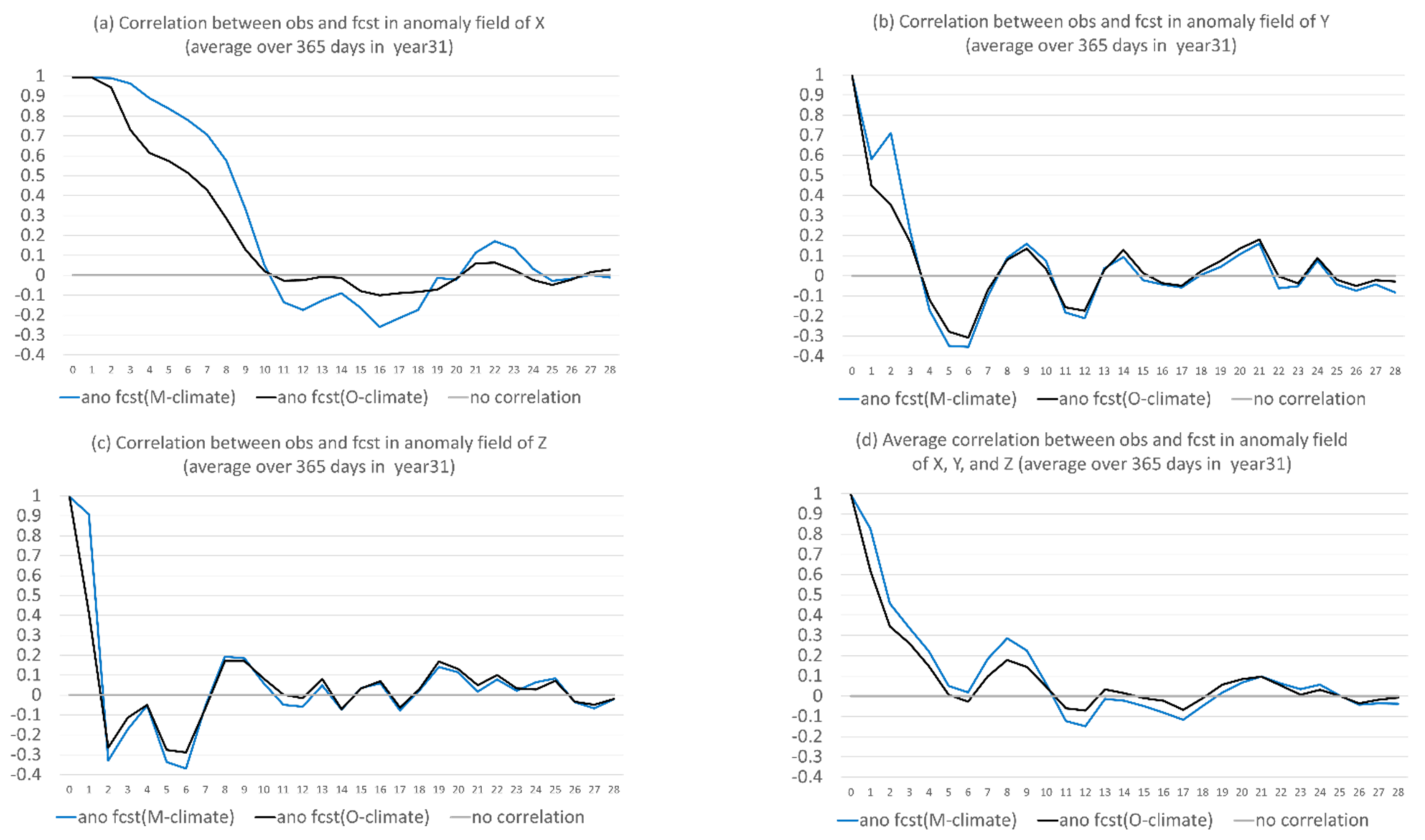
The proposed anomaly-based approach can significantly and steadily increase model forecast accuracy in both magnitude and structure (time-evolution pattern) throughout the entire forecast period (28 model days in lead time). On average of the three variables, the total forecast error was reduced by about 25%, and the correlation was boosted by about 100–200% (from negative to positive). The correlation improvement increases with the increasing of forecast length: from about 20% at day 1 to 150% at day 28.

(2)

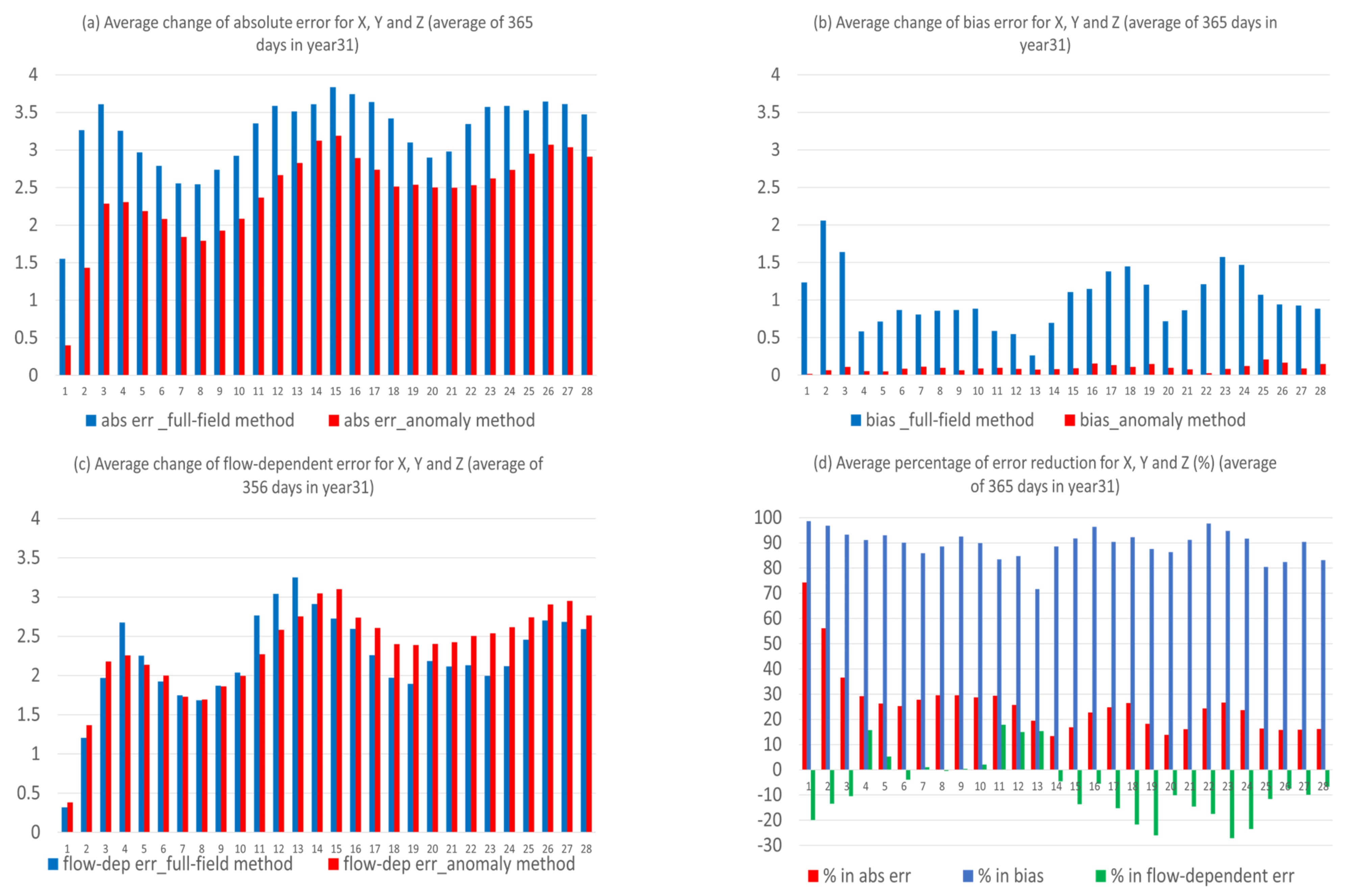
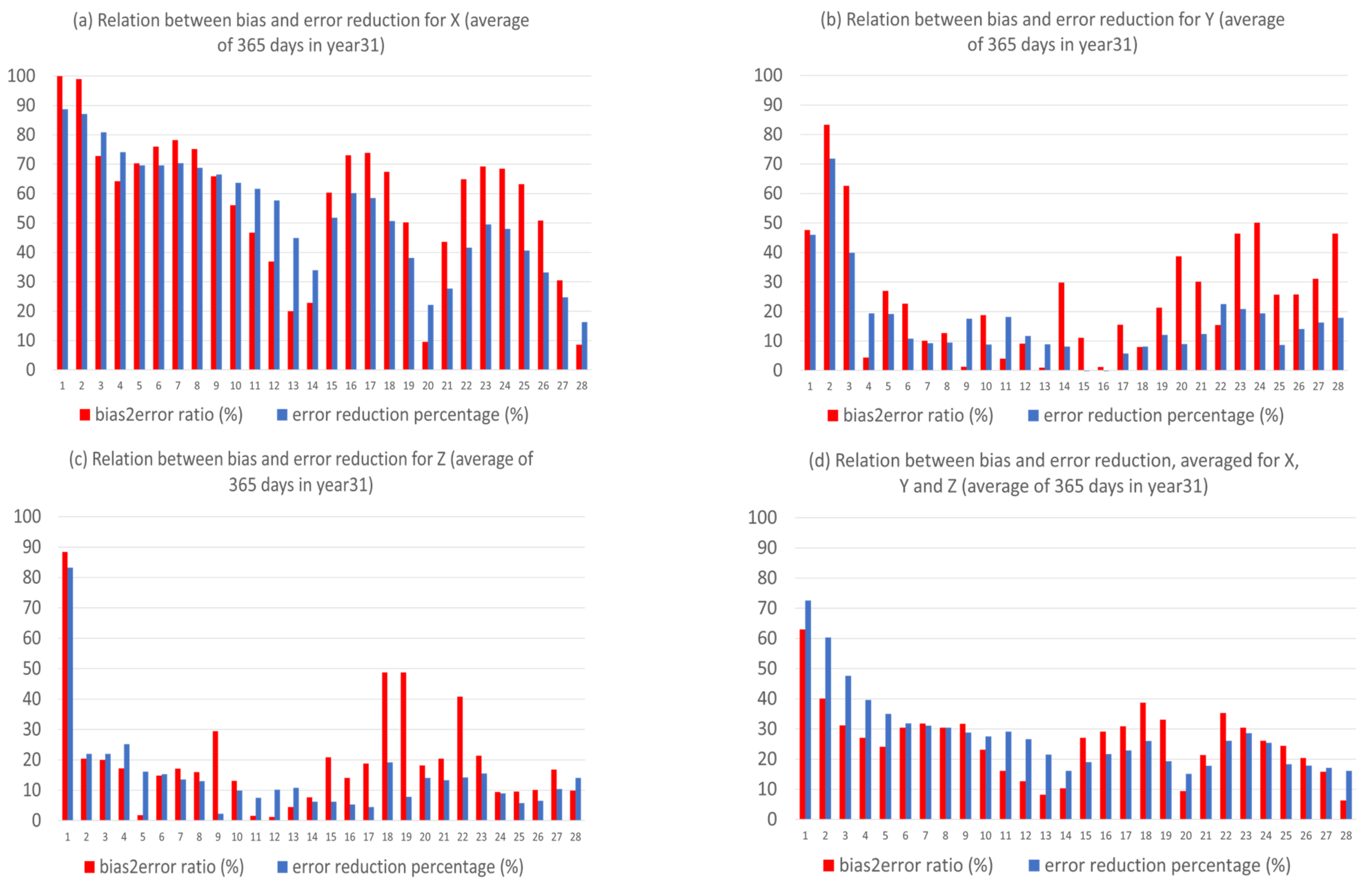
The anomaly-based method has different impacts on different types of forecast error. By decomposing the forecast error into systematic (bias) and flow-dependent (random error) errors, we found that the bias error was almost eliminated (over 90% in reduction) over the entire forecast period. However, the flow-dependent error was only slightly reduced in the first two weeks, and then became worse. On average, the reduction was about 5% over the first two weeks, and the worsening was about 15% over the last two weeks.

(3)

The reason why there is such a dramatic reduction in bias is because bias error mainly stems from model climate prediction. Since this method improves a forecast through eliminating climate forecast error, forecast improvement will be larger when model climate error or bias is larger, such as in X (about 40% in total error reduction); otherwise, it will be smaller, such as in Y and Z (about 20% and 15%). Therefore, this method is more useful for more challenging days, such as drop-off events and longer-range forecasts, when the model’s basic state (model climate) has drifted away from the true basic state (observed climate).

(4)

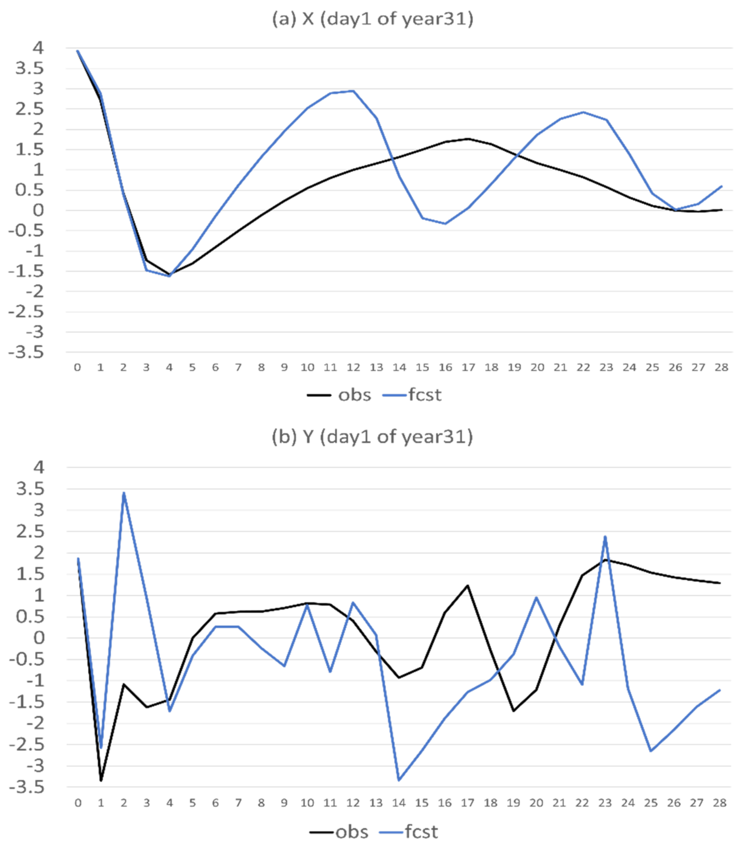
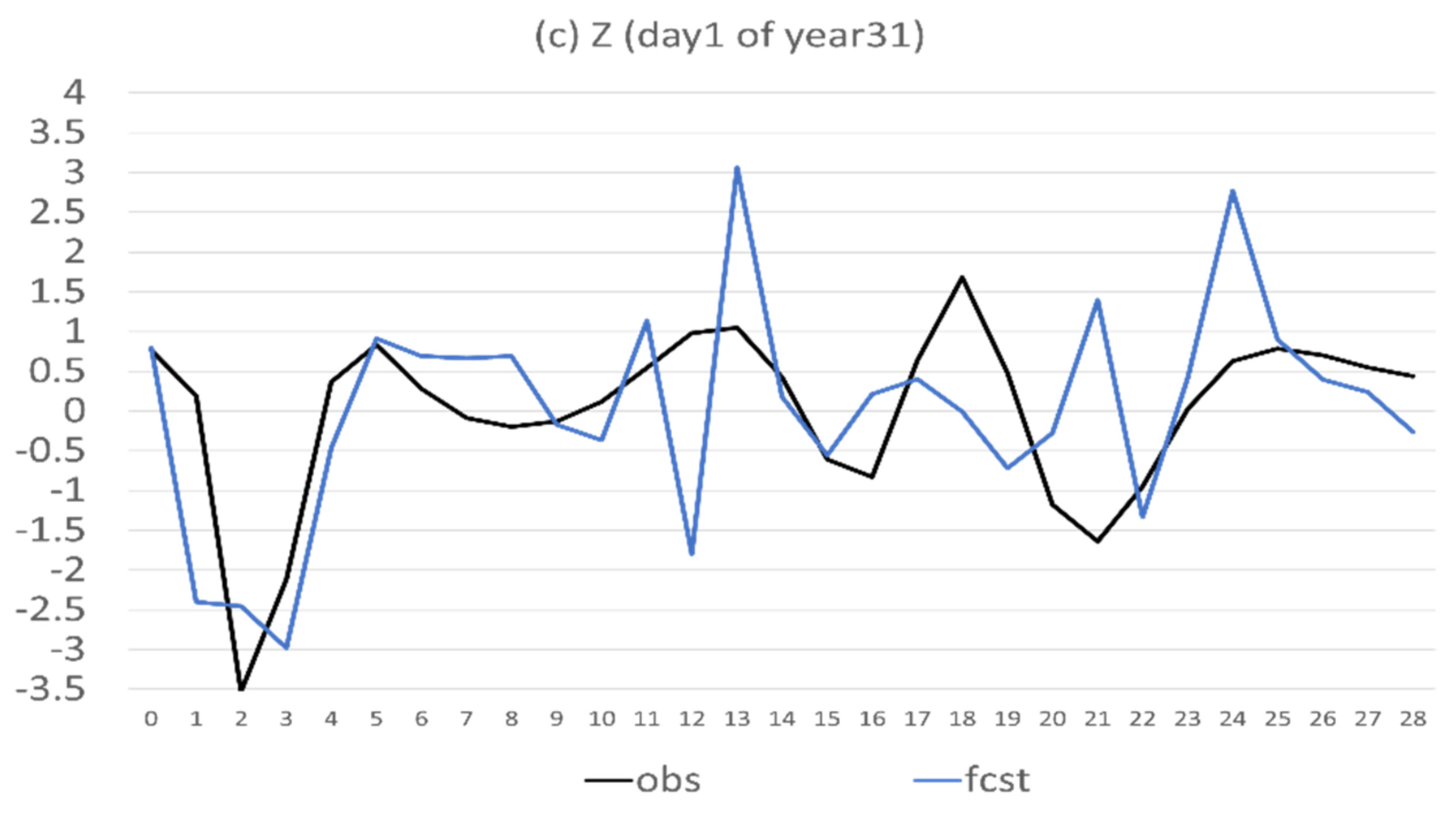
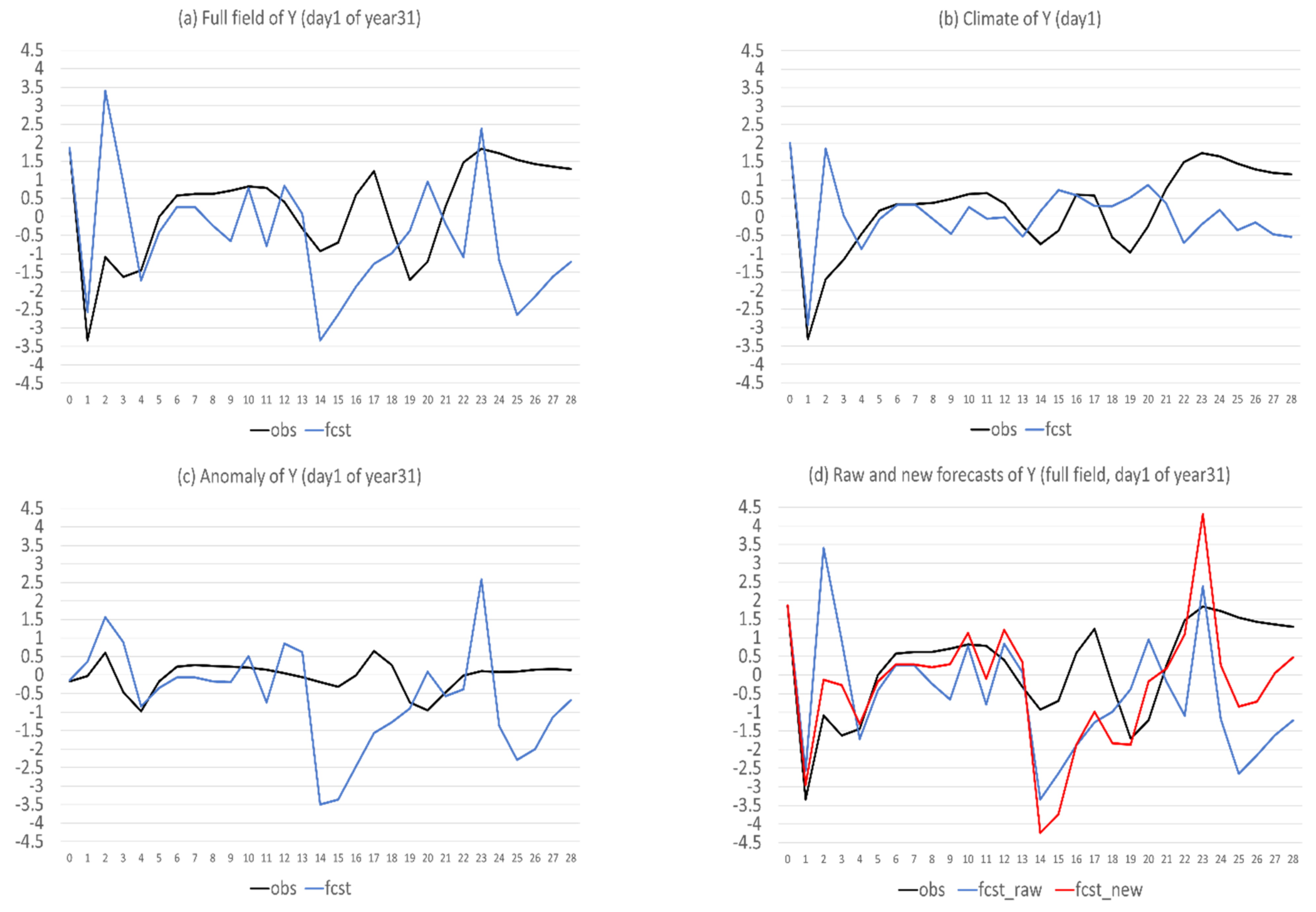
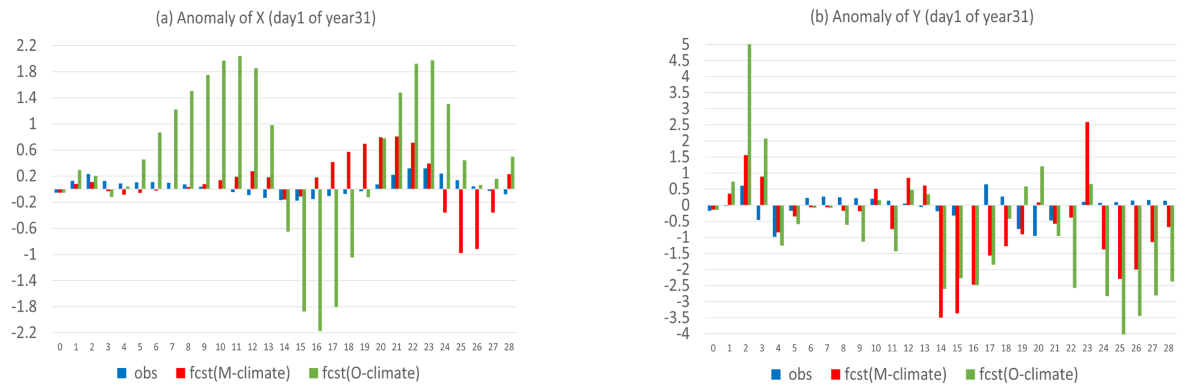
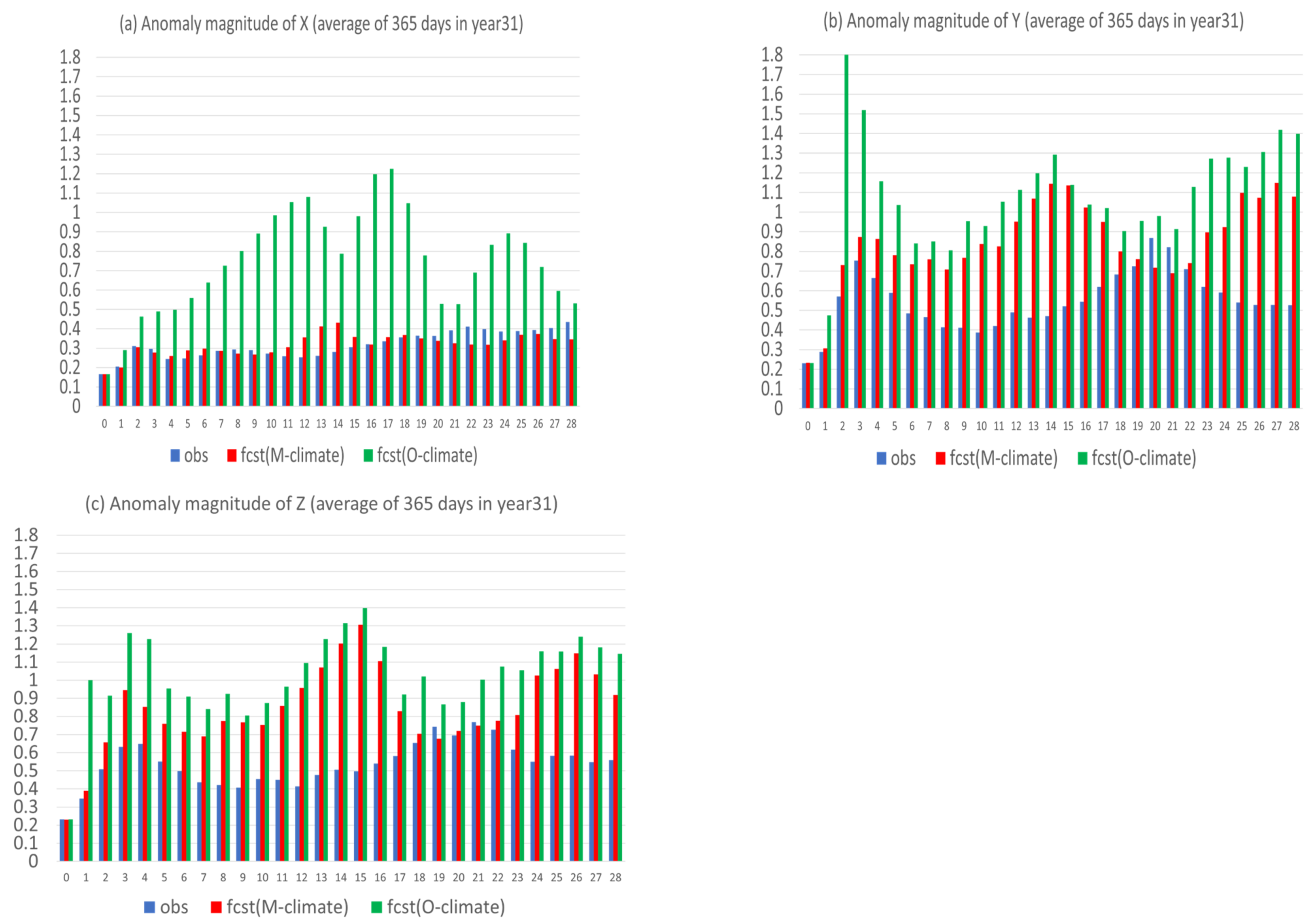
Flow-dependent error is largely associated with anomaly forecasts. As a result, flow-dependent error will be smaller when the forecast anomaly is similar to the observed anomaly, such as X (cf. Figure 3a and Figure 13a); otherwise, it will be larger when forecast anomaly is very different from observed anomaly, such as Y and Z (cf. Figure 3b–c and Figure 13b–c). In this study the predicted anomaly was much larger than the observed anomaly for Y and Z (Figure 13b–c). Therefore, their anomaly forecast errors were large, which led to large flow-dependent error in the new forecasts (Figure 6c). A consequence of this is that the flow-dependent error became even worse in many forecast hours for the new forecasts. Physically, the worsening of flow-dependent error can be explained by the “correct forecast for wrong reasons” situation that raw forecasts were accidently corrected by model bias. If the predicted anomaly magnitudes were smaller and closer to the observed (i.e., model variation is similar to the nature variation), the worsening of flow-dependent error would be to a lesser degree, and the new method would work even more effectively by reducing a larger portion of the total error.

(5)

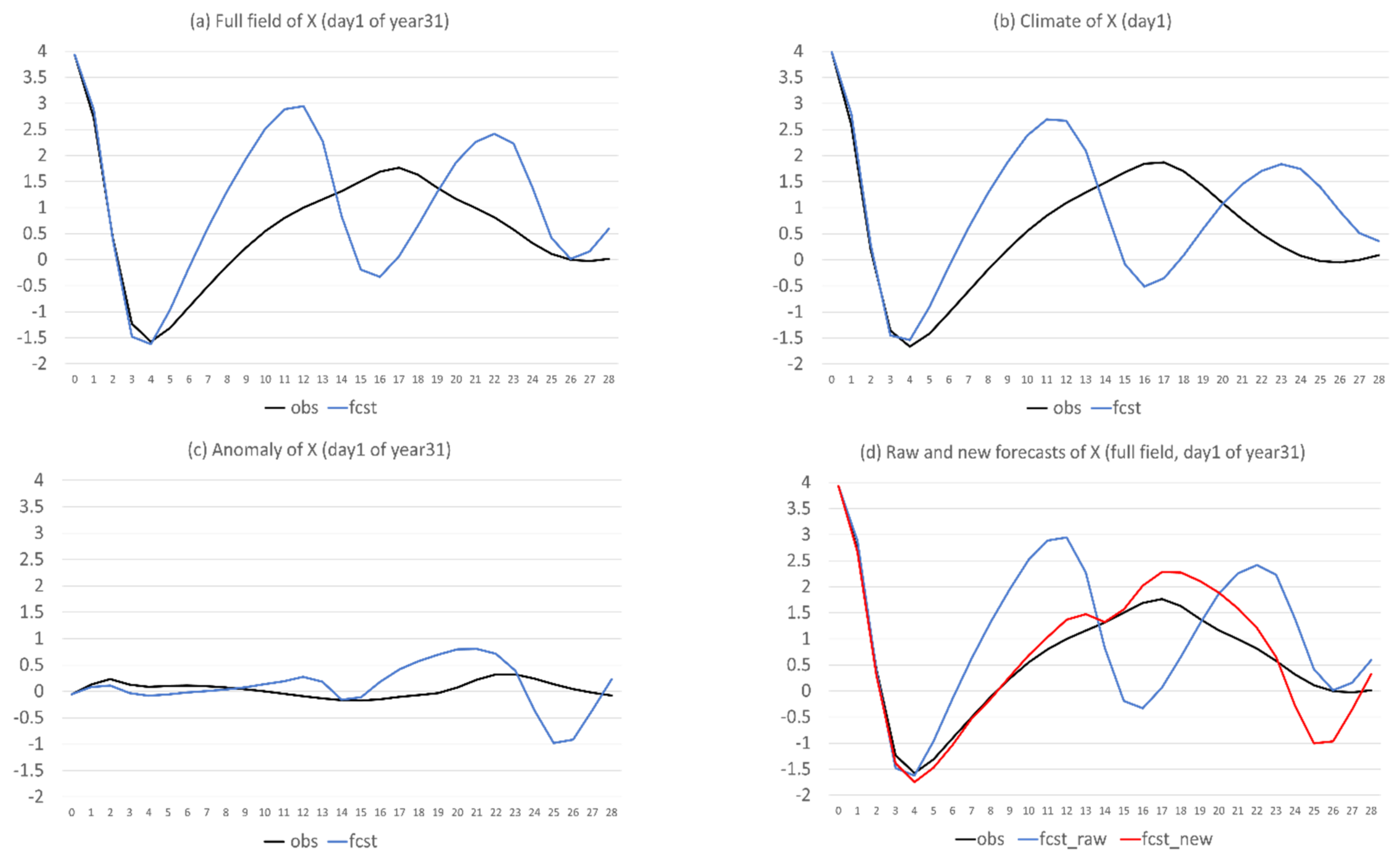
Lastly, a more accurate anomaly-forecast needs to be constructed, relative to model climate, rather than observed climate, by taking advantage of cancelling model systematic error under the perfect-model assumption.

This study suggests that the anomaly, rather than full field out of a model forecast, will be more useful to construct an accurate forecast for users. Specifically, the model climate should be replaced by the observed climate to produce a reconstructed, new, full field forecast prior to its application. As long as the model climate is different from observed climate, this anomaly-based method will be beneficial. Only when a model has no systematic bias and can perfectly predict observed climate (i.e., model climate = observed climate) will the new anomaly-based and current raw full-field based methods be equivalent to each other. Since the performance of this Lorenz model generally resembles NWP model behavior, with respect to general circulation forecasts, this work could be used as a guidance to more practical work in future. In principle, this approach can be applicable to any model-based prediction. The next step of our research will extend this work to a state-of-the-art NWP model, in order to stimulate more discussions on this new way of using model outputs. To have a spatially and temporally scale-matched field of a re-constructed new forecasts in the real NWP world, the observed climate needs to match the forecast model’s resolution in both space and time. Therefore, a good quality, high-resolution (e.g., sub-kilometer in space, at least hourly, and better sub-hourly in time) reanalysis is necessary to build an observed climate. Besides, a model reforecast should also become a standard to build model climate for any new model. Currently, a model reforecast dataset is not always available for many operational NWP models.

This new method could help model development too. First, it could technically avoid model climate drift issue immediately in a forecast by replacing the model climate with the observed climate. Secondly, it can help model developers diagnose possible model physics deficiency in the following two ways. By decomposing forecast error into climate error and anomaly error, one can see where the main error source is: climate state or anomaly variation. By examining the worsening areas of flow-dependent error to identify underlying true physics problem, since these areas are related to the “correct forecast for wrong reasons” situation (Section 3.3). Thirdly, the fact that the flow-dependent error could become worse by the new method reminds us that improving the model itself is always the top priority to fix the root causes of a forecast problem. In addition to model improvement, another way to reduce the flow-dependent error caused by unpredictable components is through an ensemble forecasting technique (Du et al., 2018 [22]). Flow-dependent bias correction method could be another way to reduce flow-dependent forecast errors (Du and DiMego 2008 [23]).

One might need to keep a few things in mind for this anomaly-based post-processing approach. Although the method should, in principle, work for all variables and scales, as long as the spatial and temporal resolutions of model and observed climates are high enough, it might work better for some than others, depending on the accuracy of the derived climate values. For example, it might work better for temperature (following Gaussian distribution with larger climatic value) than precipitation (Gamma distribution with smaller climatic value), better for synoptic scale than mesoscale phenomena, and better for longer range than shorter range forecasts. We also suggest that this method is only applied to model’s prognostic variables, not diagnostic variables. Once prognostic variables are corrected, diagnostic variables will be automatically corrected when they are derived from prognostic variables. Lastly, this method should work better in a steady-state climate than a changing climate. Changing climate could be an error source if climate change is rapid. For example, with rapid global warming, the observed climate (based on a 30-year average) might have a larger bias than the raw model forecast. Therefore, original full-field forecasts might perform better than anomaly-based forecasts when the observed climate has long-term trends. To minimize this climate-changing bias, we could use a shorter time-period (such as 10 years instead of 30 years) to derive a climatology.

As mentioned in the Introduction, the purpose of this study was to explore a new approach to extract more accurate information out of a raw model forecast rather than another bias correction method. However, since our results show that this anomaly method can almost eliminate bias error, it might be worth comparing the pros or cons of this method to other existing bias correction methods for readers’ reference. To improve a model forecast through post-processing has been a continuous effort by many in the past. Many methods have been developed, such as MOS (model output statistics) for both single model and ensemble model (Glahn and Lowry, 1972 [24]; and Gneiting et al., 2005 [25]), linear regression or weighted combination (Krishnamurti et al., 2016 [26]), Kalman-filter based decaying method (Cui et al., 2012 [27]), probability matching (Ebert, 2001 [28], Li et al., 2015 [29]; and Zhu and Luo, 2015 [30]), Bayesian model average (Raftery et al., 2017 [31]; Herr and Krzysztofowicz, 2015 [32] and 2019 [33]), neural network based method (Yuan et al., 2007 [34]), analog approach (Du and DiMego 2008 [23]; Hamill et al., 2006 [9] and 2015 [35]; and Eckel and Delle Monache, 2016 [36]), and, more recently, machine-learning based (Chan et al., 2021 [37]; and Han et al., 2021 [38]). However, all those methods are statistics-based. Because a statistical method is based on the average performance of a forecast over a past period, and probably over a region, it works only on an average sense, too, but does not necessarily work well for individual cases. For example, it might improve a forecast in one situation, spot, or time, but make it worse in another situation, spot, or time. However, this anomaly-based method has clear physical meaning, in terms of model climate and anomaly, and should improve a forecast for all individual situations, spots, and times after model-climate related error is eliminated. By the way, besides statistical approaches, a dynamical approach to correct model bias has also been explored in recent years. For example, Chen et al., (2020) [39] and Xia et al., (2019) [21] proposed a dynamical approach to debias a model forecast by correcting a model tendency term during model integration. Another advantage of this anomaly-based method is its feasibility for the user. Currently, a statistical method is a special algorithm that needs to be designed and tuned by a developer. Different variables (such as temperature and precipitation) or situations (such as short-range and long-range forecasts) need different methodologies or algorithms. Therefore, different users need different algorithms, depending on their own unique needs. However, this anomaly-based method can be a “one fits all” type of approach. It is standard and uniform for all users, variables, and situations, as long as the model and observed climates are provided together with a model forecast. This simplification will enable all users to easily post-process a model forecast by themselves before its application, which will certainly maximize the value of NWP products. Finally, it is sometimes hard, or even impossible, to explain a result coming from a statistical approach, especially a machine-learning based method, while it is easier to explain the causes of an improvement or degradation for this anomaly-based method (e.g., Section 3.3).

References

1. Gupta, A.S.; Jourdain, N.C.; Brown, J.N.; Monselesan, D. Climate drift in the CMIP5 models. J. Clim. 2013, 26, 8597–8615. [Google Scholar] [CrossRef]
2. Wang, J.; Chen, J.; Du, J.; Zhang, Y.; Xia, Y.; Deng, G. Sensitivity of Ensemble Forecast Verification to Model Bias. Mon. Weather Rev. 2018, 146, 781–796. [Google Scholar] [CrossRef]
3. Yin, L.; Fu, R.; Shevliakova, E.; Dickinson, R.E. How well can CMIP5 simulate precipitation and its controlling processes over tropical South America? Clim. Dyn. 2013, 41, 3127–3143. [Google Scholar] [CrossRef]
4. Kalnay, E.; Kanamitsu, M.; Kistler, R.; Collins, W.; Deaven, D.; Gandin, L.; Iredell, M.; Saha, S.; White, G.; Woollen, J.; et al. The NCEP/NCAR 40-Year Reanalysis Project. Bull. Am. Meteor. Soc. 1996, 77, 437–471. [Google Scholar] [CrossRef]
5. Qian, W.; Du, J.; Ai, Y. A Review: Anomaly-Based versus Full-Field-Based Weather Analysis and Forecasting. Bull. Am. Meteorol. Soc. 2021, 102, E849–E870. [Google Scholar] [CrossRef]
6. Huang, J.; Du, J.; Qian, W. A Comparison between a Generalized Beta–Advection Model and a Classical Beta–Advection Model in Predicting and Understanding Unusual Typhoon Tracks in Eastern China Seas. Weather Forecast. 2015, 30, 771–792. [Google Scholar] [CrossRef]
7. Qian, W.; Du, J. Anomaly Format of Atmospheric Governing Equations with Climate as a Reference Atmosphere. Meteorology 2022, 1, 127–141. [Google Scholar] [CrossRef]
8. Hamill, T.M.; Whitaker, J.S.; Mullen, S.L. Reforecasts: An Important Dataset for Improving Weather Predictions. Bull. Am. Meteorol. Soc. 2006, 87, 33–46. [Google Scholar] [CrossRef]
9. Lorenz, E.N. Irregularity: A fundamental property of the atmosphere. Tellus A 1984, 36A, 98–110. [Google Scholar] [CrossRef]
10. Lorenz, E.N. Can chaos and intransitivity lead to interannual variability? Tellus A 1990, 42, 378–389. [Google Scholar] [CrossRef]
11. Pielke, R.A.; Zeng, X. Long-Term Variability of Climate. J. Atmos. Sci. 1994, 51, 155–159. [Google Scholar] [CrossRef]
12. Gonzàlez-Miranda, J.M. Predictability in the Lorenz low-order general atmospheric circulation model. Phys. Lett. A 1997, 233, 347–354. [Google Scholar] [CrossRef]
13. Roebber, P.J. Climate variability in a low-order coupled atmosphere-ocean model. Tellus A 1995, 47, 473–494. [Google Scholar] [CrossRef]
14. Van Veen, L.; Opsteegh, T.; Verhulst, F. Active and passive ocean regimes in a low-order climate model. Tellus A 2001, 53, 616–627. [Google Scholar] [CrossRef]
15. Van Veen, L. Baroclinic Flow and the Lorenz-84 Model. Int. J. Bifurc. Chaos 2003, 13, 2117–2139. [Google Scholar] [CrossRef]
16. Lorenz, E.N. Chaos, Spontaneous Climatic Variations and Detection of the Greenhouse Effect. In Greenhouse-Gas-Induced Climatic Change: A Critical Appraisal of Simulations and Observations; Schlesinger, M.E., Ed.; Elsevier Science Publishers B. V.: Amsterdam, The Netherlands, 1991; pp. 445–453. [Google Scholar]
17. Shen, B.-W. Aggregated Negative Feedback in a Generalized Lorenz Model. Int. J. Bifurc. Chaos 2019, 29, 1950037. [Google Scholar] [CrossRef]
18. Wang, H.; Yu, Y.; Wen, G. Dynamical Analysis of the Lorenz-84 Atmospheric Circulation Model. J. Appl. Math. 2014, 2014, 296279. [Google Scholar] [CrossRef]
19. Shen, B.-W. Lecture #12 of Math537: Linearization Theorem; Last updated: 24 September 2020; San Diego State University: San Diego, CA, USA, 2017. [Google Scholar] [CrossRef]
20. Koh, T.-Y.; Wang, S.; Bhatt, B.C. A diagnostic suite to assess NWP performance. J. Geophys. Res. 2012, 117, D13109. [Google Scholar] [CrossRef]
21. Xia, Y.; Chen, J.; Du, J.; Zhi, X.; Wang, J.; Li, X. A Unified Scheme of Stochastic Physics and Bias Correction in an Ensemble Model to Reduce Both Random and Systematic Errors. Weather Forecast. 2019, 34, 1675–1691. [Google Scholar] [CrossRef]
22. Du, J.; Berner, J.; Buizza, R.; Charron, M.; Houtekamer, P.; Hou, D.; Jankov, I.; Mu, M.; Wang, X.; Wei, M.; et al. Ensemble Methods for Meteorological Predictions. In Handbook of Hydrometeorological Ensemble Forecasting; Duan, Q., Pappenberger, F., Thielen, J., Wood, A., Cloke, H., Schaake, J., Eds.; Springer: Berlin/Heidelberg, Germany, 2018; pp. 1–52. [Google Scholar] [CrossRef]
23. Du, J.; DiMego, G. A regime-dependent bias correction approach. In Proceedings of the 19th Conference on Probability and Statistics, New Orleans, LA, USA, 20–24 January 2008; Available online: https://ams.confex.com/ams/88Annual/webprogram/Paper133196.html (accessed on 11 September 2022).
24. Glahn, H.R.; Lowry, D.A. The Use of Model Output Statistics (MOS) in Objective Weather Forecasting. J. Appl. Meteo. 1972, 11, 1203–1211. [Google Scholar] [CrossRef]
25. Gneiting, T.; Raftery, A.E.; Westveld, A.H.; Goldman, T. Calibrated Probabilistic Forecasting Using Ensemble Model Output Statistics and Minimum CRPS Estimation. Mon. Weather Rev. 2005, 133, 1098–1118. [Google Scholar] [CrossRef]
26. Krishnamurti, T.N.; Kumar, V.; Simon, A.; Bhardwaj, A.; Ghosh, T.; Ross, R. A review of multimodel superensemble forecasting for weather, seasonal climate, and hurricanes. Rev. Geophys. 2016, 54, 336–377. [Google Scholar] [CrossRef]
27. Cui, B.; Tóth, Z.; Zhu, Y.; Hou, D. Bias Correction for Global Ensemble Forecast. Weather Forecast. 2012, 27, 396–410. [Google Scholar] [CrossRef]
28. Ebert, E.E. Ability of a poor man’s ensemble to predict the probability and distribution of precipitation. Mon. Weather Rev. 2001, 129, 2461–2480. [Google Scholar] [CrossRef]
29. Li, J.; Du, J.; Chen, C. Applications of frequency-matching method to ensemble precipitation forecasts. Meteorol. Mon. 2015, 41, 674–684. [Google Scholar]
30. Zhu, Y.; Luo, Y. Precipitation Calibration Based on the Frequency-Matching Method. Weather Forecast. 2015, 30, 1109–1124. [Google Scholar] [CrossRef]
31. Raftery, A.E.; Gneiting, T.; Balabdaoui, F.; Polakowski, M. Using Bayesian Model Averaging to Calibrate Forecast Ensembles. Mon. Weather Rev. 2017, 133, 1155–1174. [Google Scholar] [CrossRef]
32. Herr, H.D.; Krzysztofowicz, R. Ensemble Bayesian forecasting system Part I: Theory and algorithms. J. Hydrol. 2015, 524, 789–802. [Google Scholar] [CrossRef]
33. Herr, H.D.; Krzysztofowicz, R. Ensemble Bayesian forecasting system Part II: Experiments and properties. J. Hydrol. 2019, 575, 1328–1344. [Google Scholar] [CrossRef]
34. Yuan, H.; Gao, X.; Mullen, S.L.; Sorooshian, S.; Du, J.; Juang, H.H. Calibration of Probabilistic Quantitative Precipitation Forecasts with an Articial Neural Network. Weather Forecast. 2007, 22, 1287–1303. [Google Scholar] [CrossRef]
35. Hamill, T.M.; Scheuerer, M.; Bates, G.T. Analog Probabilistic Precipitation Forecasts Using GEFS Reforecasts and Climatology-Calibrated Precipitation Analyses. Mon. Weather Rev. 2015, 143, 3300–3309. [Google Scholar] [CrossRef]
36. Eckel, F.A.; Monache, L.D. A Hybrid NWP–Analog Ensemble. Mon. Weather Rev. 2016, 144, 897–911. [Google Scholar] [CrossRef]
37. Chan, M.H.K.; Wong, W.K.; Au-Yeung, K.C. Machine learning in calibrating tropical cyclone intensity forecast of ECMWF EPS. Meteorol. Appl. 2021, 26, e2041. [Google Scholar] [CrossRef]
38. Han, L.; Chen, M.; Chen, K.; Chen, H.; Zhang, Y.; Lu, B.; Song, L.; Qin, R. A Deep Learning Method for Bias Correction of ECMWF 24–240 h Forecasts. Adv. Atmos. Sci. 2021, 38, 1444–1459. [Google Scholar] [CrossRef]
39. Chen, J.; Wang, J.; Du, J.; Xia, Y.; Hongqi, L. Forecast bias correction through model integration: A dynamical wholesale approach. Q. J. R. Meteorol. Soc. 2020, 146, 1149–1168. [Google Scholar] [CrossRef]
Figure 1. A schematic diagram of the two methods: (a) model directly provides full-field forecasts, and (b) model provides anomaly only and full-field forecasts that are constructed post-processing.
Atmosphere 13 01487 g001
Figure 2. Forecasts of (a) X, (b) Y, and (c) Z on the first day of the 31st year. The vertical axis is the magnitude of X, Y, and Z, and the horizontal axis is forecast length in model days (0–28). Observed (the perfect model run) is in black and forecast (the imperfect model run) is in blue.
Atmosphere 13 01487 g002aAtmosphere 13 01487 g002b
Figure 3. Magnitude of total forecast errors (black solid line) and its decomposition into bias error (red dash line) and flow-dependent error (blue dash line) of (a) X, (b) Y, (c) Z, and (d) X + Y + Z. The vertical axis is error magnitude, and the horizontal axis is forecast length in model days (0–28). The results are averaged over the 365 days of the 31st year.
Atmosphere 13 01487 g003
Figure 4. Absolute errors of full field (black solid line), climate (red dash line), and anomaly forecasts of (a) X, (b) Y, (c) Z, and (d) X + Y + Z. The vertical axis is error magnitude, and the horizontal axis is forecast length in model days (0–28). The results are averaged over the 365 days of the 31st year.
Atmosphere 13 01487 g004
Figure 5. Correlation coefficients between forecast and truth for full field (black), climate (red), and anomaly (blue) forecasts of (a) X, (b) Y, and (c) Z. The average of (ac) is shown in (d). The vertical axis is correlation coefficient, and the horizontal axis is forecast length in model days (0–28). The results are averaged over the 365 days of the 31st year.
Atmosphere 13 01487 g005
Figure 6. Error change (the vertical axis) in magnitude from the original forecast (blue, full-field based method) to the new forecast (red, anomaly-based method) for (a) total error, (b) bias error, and (c) flow-dependent error, averaged over X, Y, and Z. The error reduction (the vertical axis) of these three types of errors is quantified as percentage in (d). The horizontal axis is forecast length in model days (0–28). The results are averaged over the 365 days of the 31st year.
Atmosphere 13 01487 g006
Figure 7. (a) Correlation coefficients (the vertical axis) of the original forecast (blue, full-field based method) and the new forecast (red, anomaly-based method), averaged over X, Y, and Z. The correlation improvement (the vertical axis) is quantified as percentage in (b). The horizontal axis is forecast length in model days (0–28). The results are averaged over the 365 days of the 31st year.
Atmosphere 13 01487 g007
Figure 8. The raw forecasts (in blue, the vertical axis) of X on the first day of the 31st year in three formats: (a) full field, (b) climate, and (c) anomaly. (d) Same as (a), but compared to the new (anomaly-method based), full field forecast of X (red). Observed (the truth run) is in black. The horizontal axis is forecast length in model days (0–28).
Atmosphere 13 01487 g008
Figure 9. A snapshot taken from the model evaluation web page at Environmental Modeling Center of National Centers for Environmental Prediction (NCEP), NOAA: https://www.emc.ncep.noaa.gov/users/verification/global/gfs/ops/grid2grid_all_models/acc/ (accessed on 11 September 2022). This is the anomaly correlation coefficient of 500 hPa geopotential height over Northern Hemisphere (20 N–80 N), valid 13 February 2021–15 March 2021 00Z. The forecast’s lead time is 5 days. Seven global models are shown.
Atmosphere 13 01487 g009
Figure 10. Same as Figure 8 but for variable Y.
Atmosphere 13 01487 g010
Figure 11. The ratio of bias error to total error (red, in percentage) and total error reduction (blue, in percentage) for (a) X, (b) Y, and (c) Z forecasts. (d) is the average of (ac). The horizontal axis is forecast length in model days (0–28). The results are averaged over the 365 days of the 31st year.
Atmosphere 13 01487 g011
Figure 12. Observed anomaly (blue) and two types of predicted anomaly, one is relative to model climate fcst (M-climate) (red) and another is relative to observed climate fcst (O-climate) (green) for (a) X, (b) Y, and (c) Z of an individual case (the first day of the year 31). The horizontal axis is forecast length in model days (0–28).
Atmosphere 13 01487 g012aAtmosphere 13 01487 g012b
Figure 13. Observed anomaly (blue) and two types of predicted anomaly, one is relative to model climate fcst(M-climate) (red) and another is relative to observed climate fcst(O-climate) (green) for (a) X, (b) Y, and (c) Z, averaged over the 365 days of year 31. The horizontal axis is forecast length in model days (0–28).
Atmosphere 13 01487 g013
Figure 14. Absolute error of the two forms of anomaly forecasts, one is with respect to model climate (fcst(M-climate) in blue) and another is with respect to observed climate (fcst(O-climate) in black) for (a) X, (b) Y, (c) Z, and (d) X + Y + Z. The vertical axis is error magnitude, and the horizontal axis is forecast length in model days (0–28). The results were averaged over the 365 days of the 31st year.
Atmosphere 13 01487 g014
Figure 15. Correlation coefficients between forecast and truth of the two forms of anomaly forecast, one is with respect to model climate (fcst(M-climate) in blue) and another is with respect to observed climate (fcst(O-climate) in black) for (a) X, (b) Y, and (c) Z. The average of (ac) is shown in (d). The vertical axis is correlation coefficient, and the horizontal axis is forecast length in model days (0–28). The results were averaged over the 365 days of the 31st year.
Atmosphere 13 01487 g015
Publisher’s Note: MDPI stays neutral with regard to jurisdictional claims in published maps and institutional affiliations.