Comparison of Urban Canopy Schemes and Surface Layer Schemes in the Simulation of a Heatwave in the Xiongan New Area

Abstract

Due to rapid growth and expansion, Xiongan New Area is at risk for heatwaves in the present and future induced by the urban heat island effect. Based on eight combined schemes, including two common WRF surface layer schemes (MM5 and Eta) and urban canopy schemes (SLAB, UCM, BEP and BEP + BEM), simulation performance for 2-m temperature, 2-m relative humidity and 10-m wind during a heatwave in July 2019 was compared and analyzed. The simulation performance is ranked from best to worst: 2-m temperature, 2-m relative humidity, 10-m wind direction and 10-m wind speed. MM5 simulate 2-m temperature and 10-m wind speed better than Eta, but 2-m relative humidity worse. MM5 coupling BEP + BEM provides the highest simulation performance for 2-m air temperature, 10-m wind direction and 10-m wind speed but the worst for 2-m relative humidity. MM5 and Eta produce nearly opposite results for wind direction and wind speed. Due to the Anxin station close to Baiyang Lake, lake-land breeze affects the simulation findings, worsening the correlation between simulated 10-m wind and observation.

1. Introduction

As global warming and the urban heat island effect develop, extreme weather and climate events hit cities more frequently [1,2,3]. Heatwaves are increasing in frequency, intensity and duration [4]. Heat-related mortality, morbidity, adverse pregnancy rates, negative mental health impacts, and heat vulnerability are all increasing with climate change [5,6]. The frequency and severity of heat waves’ effects on China’s human civilization and environment are increasing [7,8,9,10]. The North China Plain, located in the core of contemporary China, may endure deadly heat waves in the future [11]. The Xiongan New Area will become the economic hub of the Beijing-Tianjin-Hebei triangle due to its proximity to Beijing. Cheng and Li [12] analyzed the changes in average and extreme temperatures in the region using daily normalized temperature data from 1960 to 2016 and concluded that the changes in most temperature indicators in the Xiongan New Area were greater than the average changes in the neighboring Beijing-Tianjin-Hebei region and North China. In the Beijing-Tianjin-Hebei region, the Xiongan New Area currently possesses climate conditions that are conducive to urban development but will face a significant danger of high-temperature catastrophes in the future [13,14].

With the development and maturation of numerical models, simulation methods have become an essential tool for quantifying and explaining the effect of urbanization and investigating the physical process behind heatwaves. Currently, the Weather Research and Forecasting (WRF) coupled single-layer urban canopy model (UCM), multilayer urban canopy module (Building Environment Parameterization, BEP) and Building Energy Model (BEM) are widely used in urban high temperature simulation [15,16,17,18,19,20]. Loughner et al. [21] used WRF coupled with UCM to simulate a heatwave and found that decreasing commercial building heights by 8 m and residential building heights by 2.5 m results in up to 0.4 K higher daytime surface. In one of his numerical simulations in Madrid, Spain, Paz et al. [22] found that the WRF-coupled BEP configuration significantly improved the wind speed results in the built-up area, with an annual mean deviation of −0.3 m·s⁻¹ compared to the 1.6 m·s⁻¹ produced by the reference WRF operation. Giovannini et al. [23] uses numerical simulation to conclude that the urban canopy scheme BEP + BEM can well reproduce the spatial distribution of energy consumption in urban areas and its dependence on urban morphological characteristics. Since the transportation of momentum, heat, and water vapor is primarily influenced by the dynamic and thermal effects in the boundary layer [24], an increasing number of studies have been conducted to simulate and analyze wind and temperature using a variety of boundary layer parameter schemes [25,26,27]. The surface layer is located at the bottom of the boundary layer, and turbulence is the most important kind of air movement in the surface layer. The turbulent flux has a crucial role in wind speed, temperature fluctuations, carbon dioxide concentration, precipitation and latent heat release in the atmosphere [28,29,30,31]. Prasad et al. [32] evaluated the surface layer schemes Revised MM5 Monin-Obukhov (hence referred to as MM5) and Eta and found that the simulation accuracy of the WRF coupled surface layer scheme MM5 was higher. Peng et al. [33] compared the surface layer schemes MM5 and Li and found that the Li scheme has certain advantages in describing regional atmospheric stratification.

Xiongan New Area will be a new type of city model for high-quality development in the new era. During the construction process, it highlights the triple background of “green, smart, and resilient”. Its construction path and implementation in smart city, green low-carbon, resilient city, etc. The model has strong reference significance (http://www.xiongan.gov.cn/2021-08/10/c_1211325329.htm) (accessed on 3 September 2022). The thermal amplification effect of the city has a significant impact on the local city, especially in the context of high temperature weather, it is more likely to increase the high temperature and heat wave disasters. Therefore, it is necessary to adjust the urban thermal environment at the urban scale to reduce the amplification effect of urban heat islands on heat waves. However, in the existing research, only the selection of the surface layer scheme or the urban canopy scheme is generally used alone, and there are few studies on the combination between the two schemes. The optimal combination of the urban canopy scheme is of great significance to improve the simulation effect of the urban surface layer and to supplement the characteristics, formation mechanism and mitigation methods of heat waves, and can also provide reference for urban heat island regulation and thermal environment management.

2. Model Description and Experimental Design

2.1. WRF Model Description

The Weather Research and Forecasting (WRF) model is a simulation system developed for atmospheric research and numerical weather prediction. The Advanced Research WRF (ARW) model is a variant of Weather Research and Forecasting (WRF). WRF4.3.2 [34] was developed through a partnership of the Patricia Balle (HPE), Jamie Bresch (NCAR), Jordan Schnell (NOAA), Yaping Shao (Universität zu Köln), Martina Klose (Karlsruhe Institute of Technology), Piotr Kasprzyk (IETU Katowice), Theodore M. Giannaros (National Observatory of Athens, Greece). It was used in this work to simulate the temperature, surface wind and relative humidity in the Xiongan New Area. This research configures the WRF model with three nested domains (shown in Figure 1). This simulation employs a three-layer nesting method. The location of the simulation center is 39° N and 116° E. The grid point sizes (grid resolution) for each domain are 81 × 81 (27 km), 121 × 121 (9 km), and 181 × 181 (3 km). The key physical choices considered for this study were configured as follows: WRF single-moment 3-class (WSM3) scheme [35]; Rapid Radiative Transfer Model (RRTM) Longwave [36]; Dudhia shortwave radiation scheme [37]; Noah land-surface module [38].

The BEP scheme and BEP + BEM scheme can only be used with Mellor-Yamada-Janjic (MYJ) PBL, Yonsei University (YSU) PBL and Boulac PBL in the WRF (V4.3.2) model. The MYJ scheme and YSU scheme can only be used with Eta and Revised MM5 Monin-Obukhov (hence referred to as MM5), respectively. The MM5 scheme and Eta scheme, which are both reasonably prevalent schemes, can be used with Boulac PBL. The MM5 scheme is a significant advance over its predecessor, the M-O similarity theory-based MM5 scheme [39]. The Eta scheme [40,41,42] is also based on the M-O similarity hypothesis. Under stable and unstable layers, the scheme uses the stability functions provided by Holtslag and De Bruin [43] and Paulson [44], respectively, to calculate the surface layer turbulent flux iteratively. To simulate the Xiongan New Area, urban canopy schemes (SLAB(urban canopy schemes not selected), UCM, BEP, BEP + BEM) and surface layer schemes (MM5, Eta) were selected to form 8 parametric combination schemes. The eight parameter combinations are listed in

Table 1. Physical parameterization configuration of the simulation.

Scheme	SIM1	SIM2	SIM3	SIM4	SIM5	SIM6	SIM7	SIM8
urban canopy	SLAB	UCM	BEP	BEP + BEM	SLAB	UCM	BEP	BEP + BEM
surface layer	MM5	MM5	MM5	MM5	Eta	Eta	Eta	Eta

.

2.2. Description of Study Areas

The planning scope includes the administrative districts of Xiongxian County, Rongcheng County and Anxin County (including Baiyang Lake), Weizhou Town, gougezhuang Town, qijianfang Township and Longhua Township of Gaoyang County in Renqiu City, with a planning area of 1770 square kilometers (http://www.xiongan.gov.cn/2018-04/21/c_129855813_2.htm) (accessed on 3 September 2022).

2.3. Description of Study Data

The observation data used in this study came from the national basic automated weather stations of the China Meteorological Administration and consist of 2-m temperature, 2-m relative humidity, and 10-m wind speed and direction. These data are used to evaluate the performance of 8 combined parameterization schemes, and comprehensive comparisons are performed through data lists, line graphs, Taylor charts, and wind rose graphs. ERA5 is the driving field for the numerical experiments. ERA5 is the fifth generation of ECMWF reanalysis covering the past 4 to 7 decades of global climate and weather with a horizontal resolution of 0.25° × 0.25°.

From 2–4 July 2019, the Xiongan New Area was affected by a heatwave, and the center of the heatwave gradually moved from the southern part of Beijing-Tianjin-Hebei to the central and eastern parts (Figure 2). The highest temperatures in the Xiongan New Area on 2–4 July were 40.4 °C, 40.2 °C and 41.5 °C, respectively. Raei et al. [45] believe that the definition of a heatwave is the maximum temperature exceeds the 90th percentile of the long-term JJA daily temperature record over a 15-day window (from 7 days ahead to 7 days after the day of interest) for at least three consecutive days. In China, when the daily maximum temperature reaches or exceeds 35 °C, it is generally called high temperature, and the high temperature weather process for several consecutive days (at least three days) is called a heatwave. This is a case of a heatwave event.

2.4. Statistical Metrics

In this work, the correlation coefficient (R), the mean bias (MB), the standard deviation (STDE), the root mean square error (RMSE), and the index of agreement (IOA) are used to evaluate and analyze the simulation results of the model. Standardization is applied to the standard deviation and root mean square error. In addition, the Taylor diagram is used to demonstrate the accuracy of the simulation results. Taylor [46] presented a diagram to evaluate the model’s relative advantages and overall performance. It provided a concise summary of the diagram’s principle and established the relationship between the correlation coefficient (R) between the simulated field and the observed field, the root mean square error (RMSE) of the center, the standard deviation (σ_f) of the simulated field and the standard deviation (σ_r) of the observed field. They are displayed on a polar map. RMSE is a part of the traditional root mean square error RMS that may distinguish the difference between the mean value of the simulated field and the observed field, allowing for a more accurate evaluation of the model’s advantages and performance. Moazenzadeh [47] and Wadoux [48] have utilized Taylor diagrams in several applications.

The formulae for calculation are (1)–(5).

$$\mathrm{R}=\frac{\frac{1}{\mathrm{N}}{\sum }_{\mathrm{n}=1}^{\mathrm{N}}\left({\mathrm{f}}_{\mathrm{n}}-\overline{\mathrm{f}}\right)\left({\mathrm{r}}_{\mathrm{n}}-\overline{\mathrm{r}}\right)}{{\mathsf{\sigma }}_{\mathrm{f}}{\mathsf{\sigma }}_{\mathrm{r}}}$$

(1)

$$\mathrm{STDE}={\left(\frac{1}{N}{\displaystyle \sum }_{n=1}^N{\left(x_n-\overline{x}\right)}^2\right)}^{\frac{1}{2}}$$

(2)

$$\mathrm{MB}=\frac{{\sum }_{n=1}^N\left(f_n-r_n\right)}{N}$$

(3)

$$\mathrm{IOA}=1.0-\frac{{\sum }_{n=1}^N{\left(r_n-f_n\right)}^2}{{\sum }_{n=1}^N{\left(\left|f_n-\overline{r}\right|+\left|r_n-\overline{r}\right|\right)}^2}$$

(4)

$$\mathrm{RMSE}={\left\{\frac{1}{N}{\displaystyle \sum }_{n=1}^N{\left[\left(f_n-\overline{f}\right)-\left(r_n-\overline{r}\right)\right]}^2\right\}}^{\frac{1}{2}}$$

(5)

3. Results

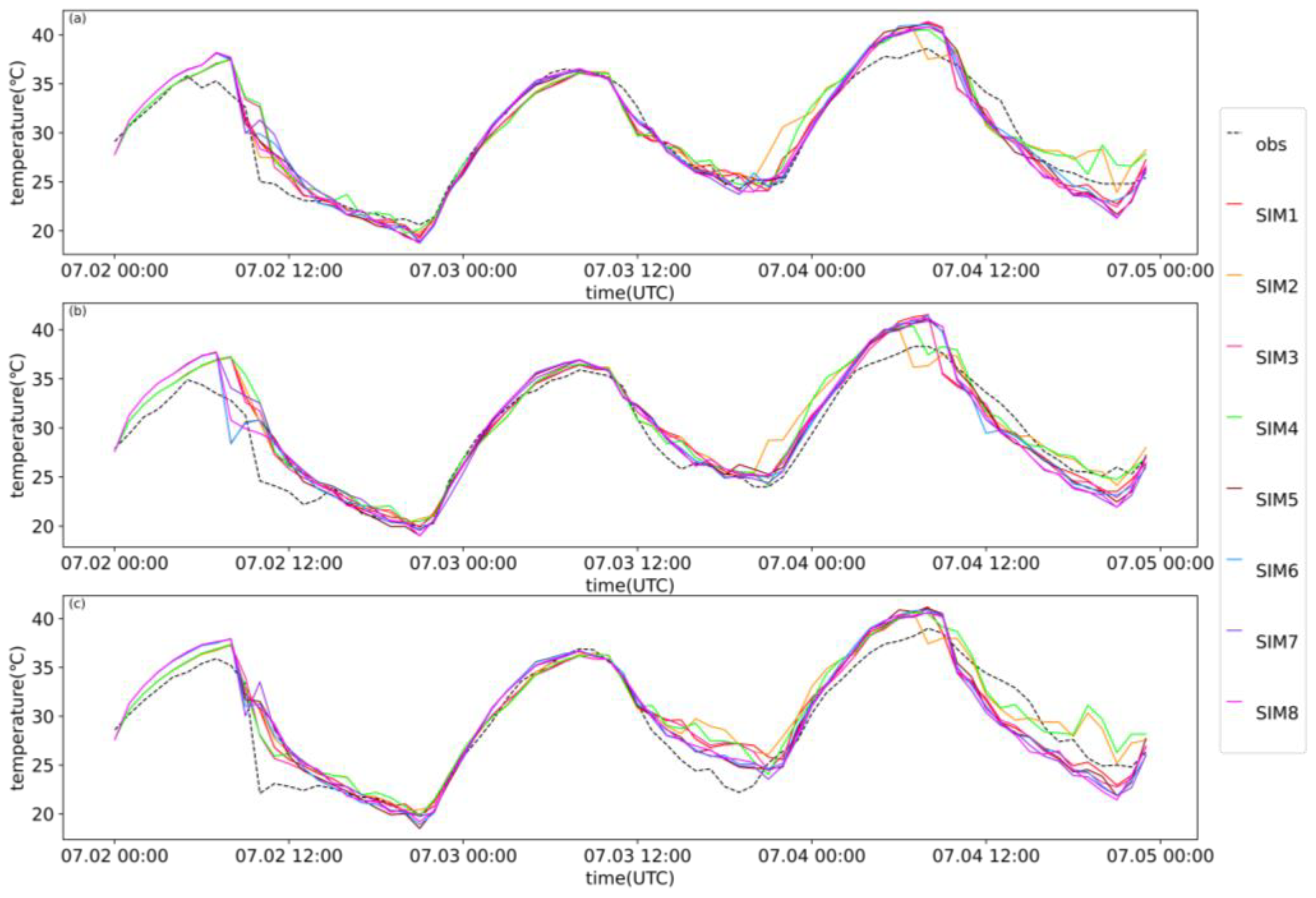
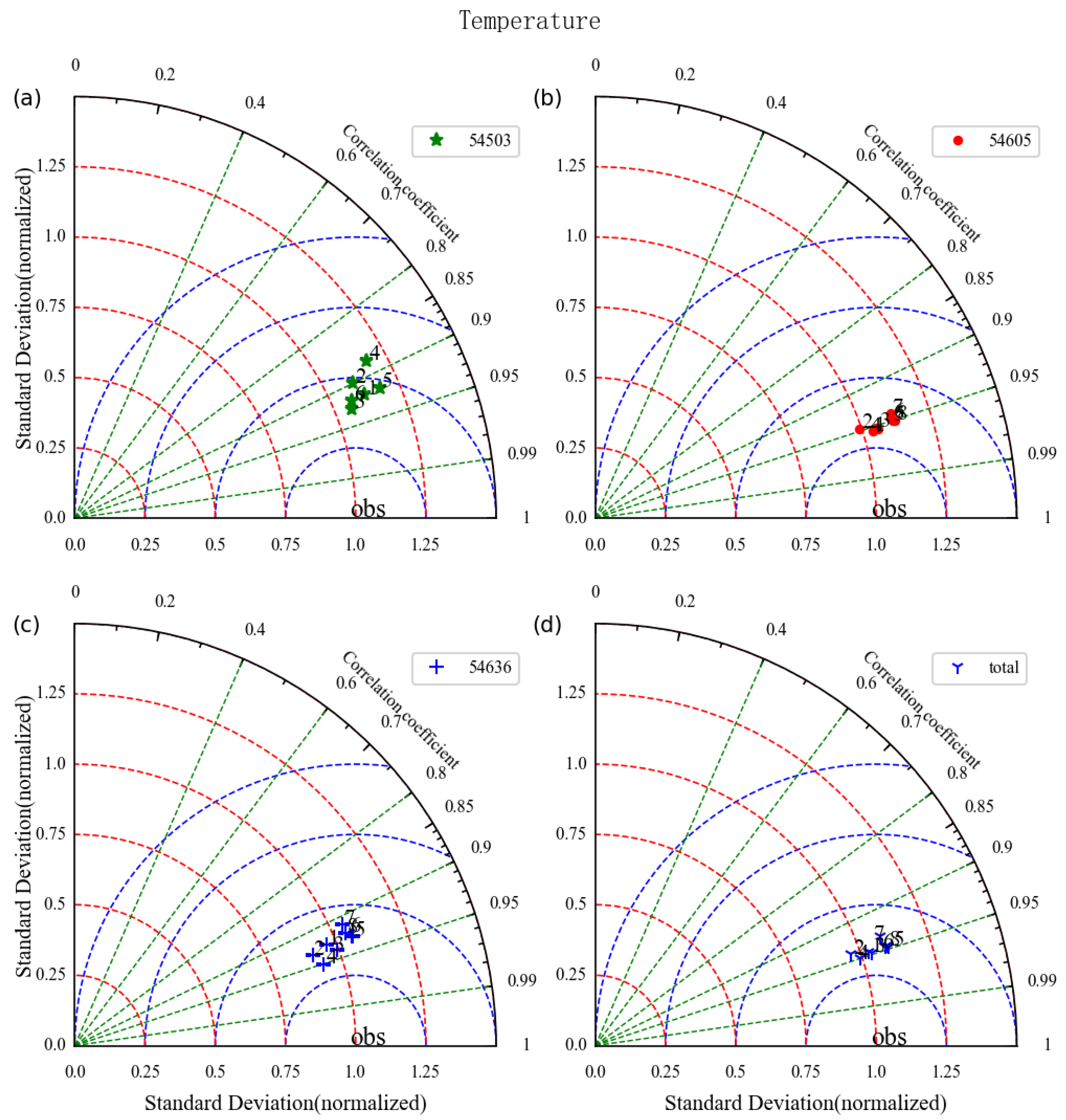
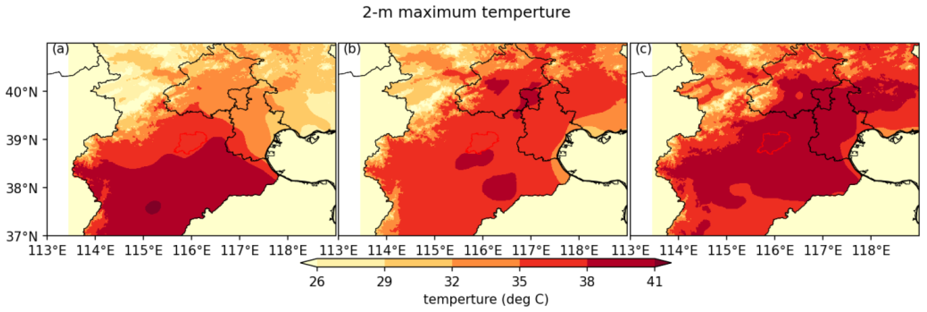
3.1. 2-m Temperature

As shown in Figure 3, all 8 experiments are capable of simulating the temperature variation, and the daytime simulated temperature is higher than the measured one, while the opposite during the nighttime. In the first 14 h of model operation, the simulated temperature is on the high side, but after 14:00 on 2–July (universal time, the following times are all UTC), the simulated values are close to the observed values, especially on 2–July. From 14:00 to 04:00 on 3–July, the simulation bias is minor, indicating that after a period of time, the model reaches a stable state, and the simulated temperature is closer to the observed value. According to the maximum temperature, the simulated maximum temperature is higher than the observed value, and the simulated time is 1–2 h away from the observation time. Overall, the maximum temperature simulated by SIM1-SIM4 (both with MM5) is closer to the observed value than the maximum temperature simulated by SIM5-SIM8 (both with Eta). In the same urban canopy scheme, the maximum temperature simulated by the MM5 scheme is more accurate than that simulated by the Eta scheme. The simulation value of the ETA scheme is lower for the simulation of the minimum temperature.

As shown in

Table 2. The 2-m temperature in the Xiongan New Area from observations and eight combined scheme simulations.

Station	Measure	SIM1	SIM2	SIM3	SIM4	SIM5	SIM6	SIM7	SIM8
54,503	IOA	0.98	0.97	0.98	0.97	0.98	0.98	0.97	0.98
	MB/°C	−0.01	0.45	−0.01	0.58	0.02	0.17	0.00	0.03
	R	0.96	0.95	0.96	0.95	0.97	0.97	0.95	0.97
	STDE	1.07	1.00	1.08	1.02	1.13	1.11	1.11	1.13
	RMSE	0.28	0.31	0.31	0.32	0.30	0.30	0.34	0.29
54,605	IOA	0.97	0.96	0.97	0.97	0.97	0.97	0.96	0.97
	MB/°C	0.71	0.99	0.68	1.04	0.63	0.58	0.61	0.63
	R	0.95	0.95	0.95	0.95	0.95	0.95	0.94	0.95
	STDE	1.06	0.99	1.05	1.04	1.12	1.11	1.12	1.12
	RMSE	0.32	0.32	0.32	0.31	0.35	0.36	0.38	0.35
54,636	IOA	0.96	0.95	0.97	0.96	0.96	0.96	0.95	0.96
	MB/°C	0.60	1.19	0.40	1.18	0.49	0.46	0.37	0.47
	R	0.93	0.93	0.94	0.95	0.93	0.93	0.91	0.92
	STDE	0.97	0.91	0.99	0.93	1.06	1.06	1.04	1.04
	RMSE	0.37	0.36	0.35	0.31	0.39	0.39	0.43	0.40
total	IOA	0.97	0.96	0.97	0.97	0.97	0.97	0.96	0.97
	MB/°C	0.44	0.88	0.36	0.94	0.38	0.41	0.33	0.37
	R	0.95	0.94	0.95	0.95	0.95	0.95	0.93	0.95
	STDE	1.03	0.97	1.04	0.99	1.10	1.09	1.09	1.09
	RMSE	0.33	0.34	0.33	0.32	0.35	0.35	0.39	0.36

, the IOA in the Xiongan New Area is greater than 0.95, suggesting that the 2-m temperature simulated by these 8 combined schemes is in good agreement. Except for Rongcheng’s SIM1 and SIM3, all other combined schemes result in a 0.01 °C increase in simulated temperature. Among the three areas, Rongcheng has the lowest MB and RMSE, and the simulation of the 2-m temperature is closest to the observed value. From the standpoint of the total MB, the average temperature simulated by the eight combined schemes is high (MB is all positive). Combined with Figure 3, it is evident that the simulated daytime temperature is high, while the nighttime temperature is low. Although the deviations of schemes SIM1-4 are larger than those of schemes SIM5-8 and the temperature MB simulated by the Eta scheme is smaller, the RMSE indicates that the MM5 scheme is better than the Eta scheme under the same canopy parameterization scheme. Comparing the sensible heat flux variation at each site (Figure 4), the sensible heat fluxes of the eight combined schemes are not significantly different. SIM1-4 (MM5) is less than the simulated value of SIM5-8 (Eta), and the calculated heat flux value of the Eta scheme is greater than that of the MM5 scheme, which also impacts the features of changes over time. SIM5-8 has a greater simulated temperature than SIM1-4; hence, the MB is larger. This is consistent with Xie’s [49] finding that the surface heat exchange coefficient Ch calculated by the Eta scheme and MM5 scheme influences the simulated results for the 2 m temperature.

The correlation coefficients (R) of the temperature simulations (Table 2) in Rongcheng, Xiongxian, and Anxin range from 0.91 to 0.98, and the overall correlation coefficient (R) is greater than 0.93. A good positive correlation exists between the simulated temperature values and the observed values. SIM1-4 has a lower overall RMSE than SIM5-8. The MM5 scheme is more accurate than the Eta scheme for simulating temperature. Figure 5 demonstrates that SIM7 has the poorest simulation, both when comparing the three regions independently and when comparing the three regions together. In addition to low simulation accuracy in Rongcheng, SIM4 performs best in Xiongxian, Anxin and overall. The BEP + BEM scheme provides a more detailed description of the process in the urban canopy, which reflects the influence of urban turbulence at different levels. Moreover, indoor human activities and the influence of home equipment on the mixing of indoor and outside air would change the ambient temperature to some extent. The combination of the BEP + BEM and MM5 schemes provides the most accurate temperature simulation.

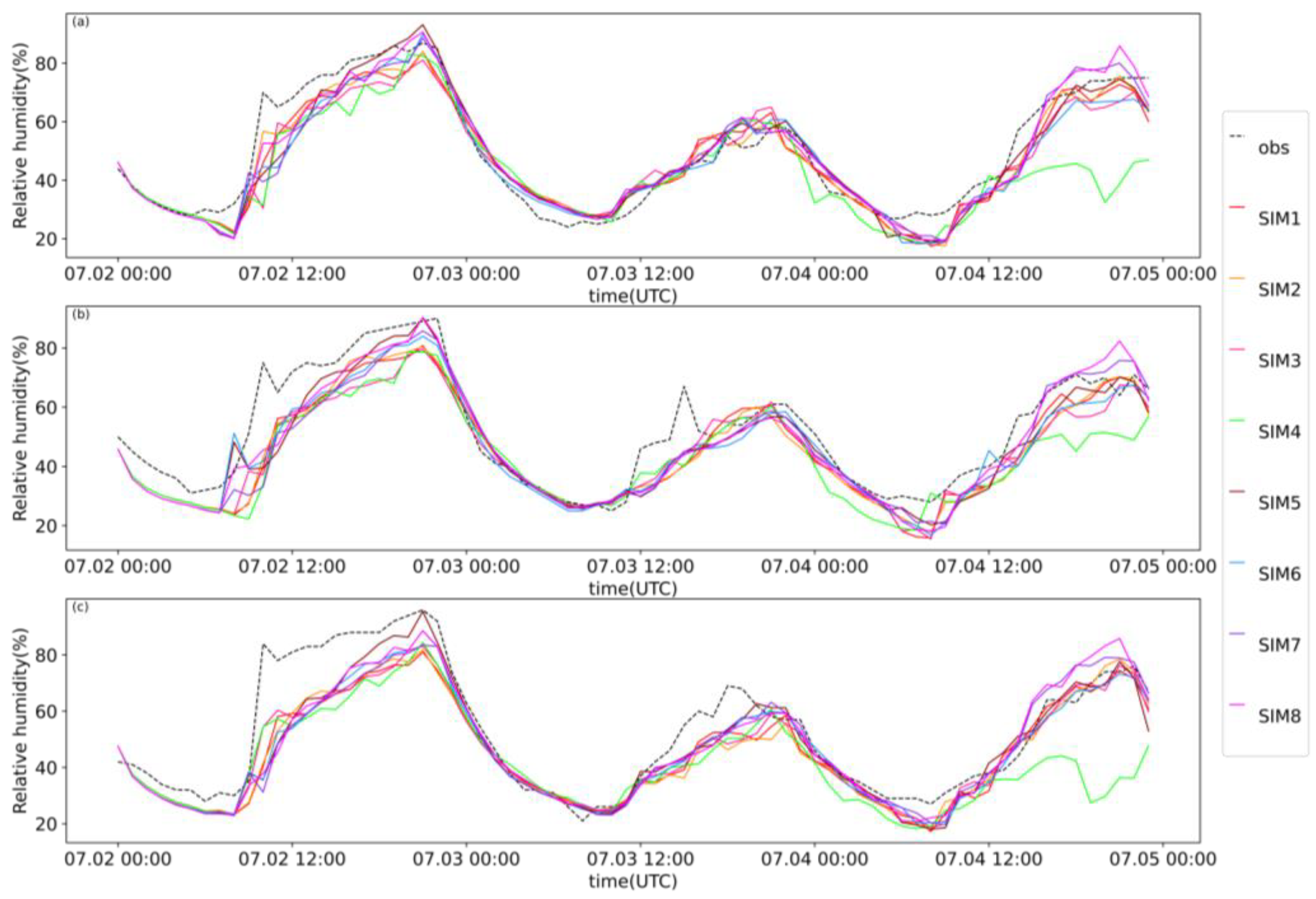
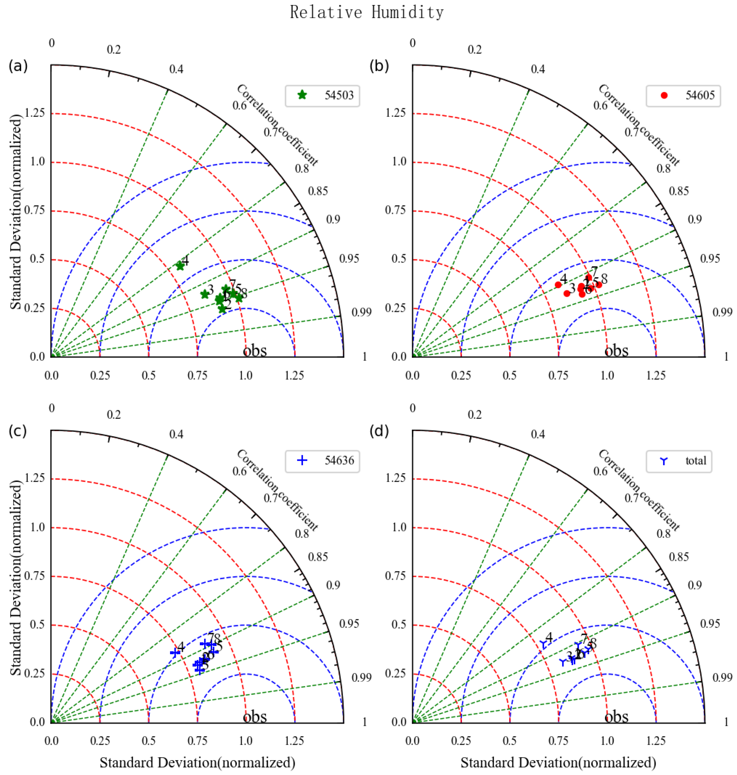
3.2. 2-m Relative Humidity

During the early stage of the model operation, the simulated relative humidity has a large MB, with the value between 14 and 20 on 2–July being notably low (Figure 6). After 20:00 on 2–July, the model stabilized, and the simulated relative humidity closely matched the observed value. The 8 combined schemes are capable of simulating the evolution of relative humidity, with superior performance for the daily relative humidity variations. However, from 16:00 to 23:00 on 4–July, SIM4 shows a large deviation, and its performance is poor.

Each scheme has a good capacity to simulate relative humidity in Xiongan New Area, where the IOA is more than or equal to 0.85 (

Table 3. The 2-m relative humidity in the Xiongan New Area from observations and eight combined scheme simulations.

Station	Measure	SIM1	SIM2	SIM3	SIM4	SIM5	SIM6	SIM7	SIM8
54,503	IOA	0.97	0.98	0.95	0.87	0.97	0.96	0.96	0.98
	MB/%	−2.16	−2.10	−2.64	−6.35	−1.46	−2.81	−1.30	−0.74
	R	0.95	0.96	0.93	0.82	0.94	0.94	0.93	0.95
	STDE	0.91	0.91	0.85	0.81	0.99	0.92	0.96	1.01
	RMSE	0.32	0.27	0.38	0.58	0.33	0.33	0.36	0.30
54,605	IOA	0.93	0.93	0.92	0.88	0.95	0.94	0.93	0.95
	MB/%	−6.39	−6.67	−7.16	−8.86	−5.28	−6.10	−5.35	−4.60
	R	0.92	0.93	0.92	0.89	0.93	0.94	0.91	0.93
	STDE	0.94	0.93	0.85	0.83	0.98	0.93	0.99	1.03
	RMSE	0.39	0.38	0.39	0.45	0.37	0.35	0.42	0.38
54,636	IOA	0.92	0.93	0.94	0.85	0.94	0.93	0.93	0.93
	MB/%	−6.86	−6.87	−6.17	−10.79	−5.16	−6.05	−5.06	−4.67
	R	0.93	0.93	0.94	0.87	0.92	0.92	0.89	0.90
	STDE	0.81	0.82	0.81	0.73	0.91	0.85	0.89	0.92
	RMSE	0.39	0.39	0.36	0.51	0.40	0.39	0.46	0.44
total	IOA	0.94	0.94	0.93	0.86	0.95	0.95	0.94	0.95
	MB/%	−5.14	−5.21	−5.32	−8.67	−3.97	−4.98	−3.90	−3.34
	R	0.93	0.93	0.93	0.85	0.93	0.93	0.90	0.92
	STDE	0.88	0.88	0.83	0.79	0.95	0.89	0.94	0.98
	RMSE	0.38	0.37	0.39	0.53	0.38	0.37	0.43	0.39

). The simulated relative humidity MB is less than zero, but the observed value is greater. Similar to the temperature, Rongcheng has the lowest MB and least simulated deviation among the three regions. The correlation between the simulated value and the observed value is good (R: 0.82–0.96) but not as good as the correlation of the 2-m temperature simulation, and these parameterization schemes are preferable for the temperature simulation. SIM4 has the largest RMSE, and SIM7 has the second-largest RMSE. The combination of BEP + BEM and MM5 has the best performance in simulating temperature but the lowest performance in simulating relative humidity. SIM2 and SIM6 have the closest simulated values to the observed values, while SIM4 and SIM7 have the farthest simulated values from the observed values. Under the same near-surface scheme, the UCM scheme is the best in simulating relative humidity (Figure 7).

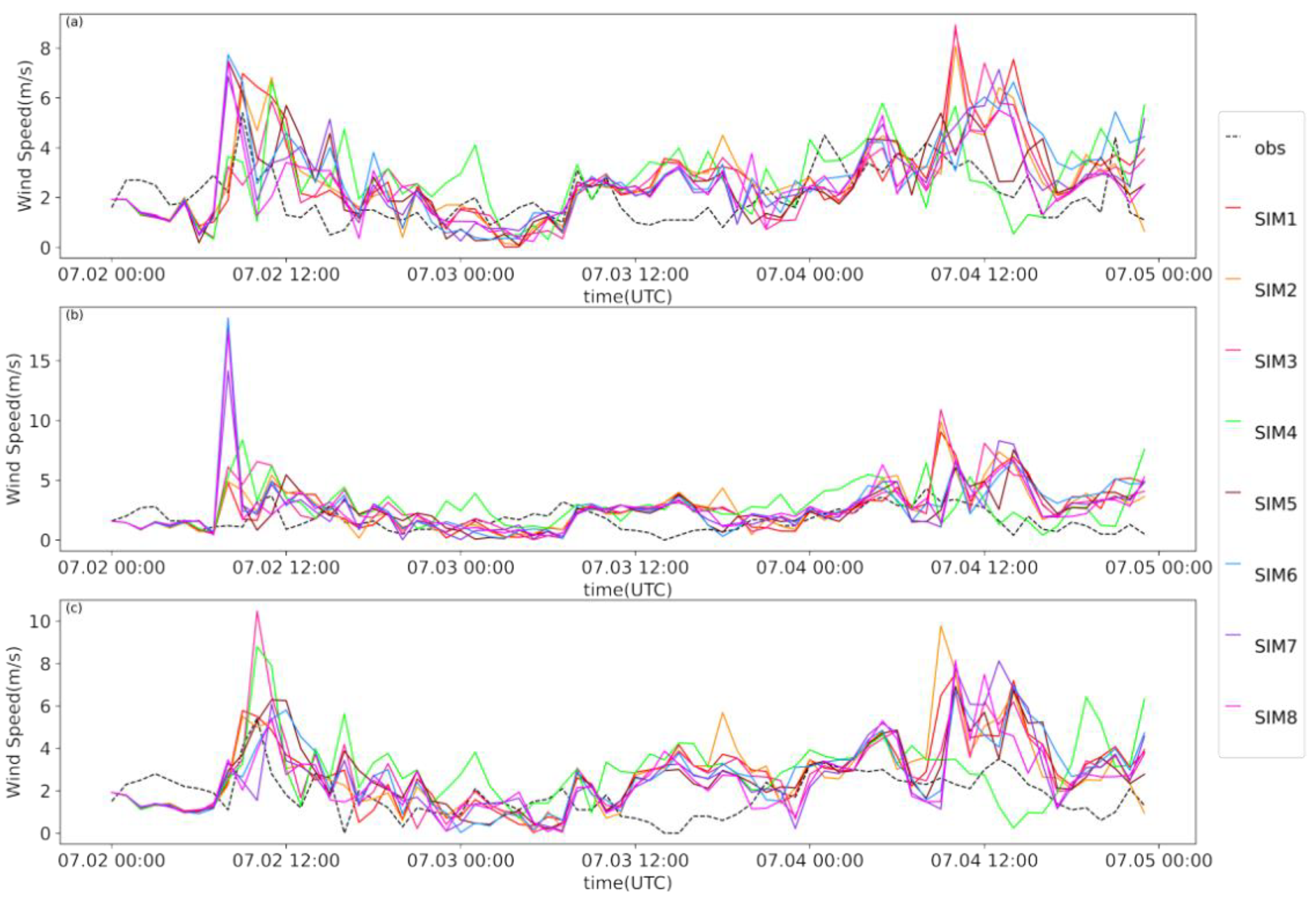
3.3. 10-m Wind Speed and Direction

From the hourly variation in wind speed (Figure 8), all eight combined schemes can show fluctuations in wind speed, but the simulated wind speed peak is slightly ahead of schedule, and the bias of the larger wind speed simulation is larger, with Anxin deviating the most from the simulated value of the daytime maximum wind speed on 2–July (Figure 8b).

Each time the wind speed increases, the model needs several hours of adjustment to get closer to the observed value, whereas when the wind speed is low, the simulated wind speed is close to the observed value, thereby enhancing the simulation capability of the 8 combined schemes for low wind speeds.

Table 4. The 10-m wind speed in the Xiongan New Area from observations and eight combined scheme simulations.

Station	Measure	SIM1	SIM2	SIM3	SIM4	SIM5	SIM6	SIM7	SIM8
54,503	IOA	0.57	0.60	0.48	0.51	0.59	0.55	0.53	0.53
	MB/(m·s−1)	0.67	0.62	0.49	0.65	0.46	0.71	0.54	0.35
	R	0.41	0.43	0.25	0.23	0.37	0.35	0.31	0.29
	STDE	1.66	1.48	1.48	1.32	1.42	1.57	1.41	1.26
	RMSE	1.55	1.39	1.56	1.46	1.41	1.54	1.46	1.36
54,605	IOA	0.41	0.43	0.43	0.47	0.20	0.25	0.28	0.28
	MB/(m·s−1)	0.92	0.95	1.10	1.11	0.95	1.07	0.87	0.96
	R	0.14	0.18	0.22	0.25	−0.08	0.00	0.00	0.04
	STDE	1.87	1.89	2.03	1.69	2.49	2.52	2.24	2.37
	RMSE	1.99	1.97	2.05	1.74	2.76	2.71	2.45	2.53
54,636	IOA	0.55	0.53	0.58	0.44	0.52	0.48	0.45	0.52
	MB/(m·s−1)	0.96	0.92	0.93	1.11	0.88	0.91	0.76	0.62
	R	0.37	0.37	0.44	0.12	0.34	0.25	0.23	0.29
	STDE	1.60	1.75	1.76	1.57	1.56	1.57	1.74	1.52
	RMSE	1.54	1.66	1.60	1.76	1.55	1.64	1.80	1.55
total	IOA	0.51	0.52	0.49	0.47	0.40	0.41	0.41	0.41
	MB/(m·s−1)	0.85	0.83	0.84	0.96	0.76	0.89	0.72	0.65
	R	0.31	0.32	0.29	0.19	0.16	0.18	0.16	0.17
	STDE	1.69	1.68	1.73	1.51	1.83	1.88	1.78	1.72
	RMSE	1.67	1.66	1.73	1.64	1.94	1.97	1.89	1.84

demonstrates that the wind speed simulation performance of the eight combined schemes is low (IOA: 0.20–0.60), with Anxin having the worst performance (IOA: 0.20–0.47). The total R of the simulated wind speed in Xiongan is 0.16~0.32, and the correlation is very weak, particularly for the Anxin schemes SIM6 and SIM7, which are close to 0, and SIM5, which has a negative correlation. The MBs of the 8 combined schemes are all positive, suggesting that the simulation of the 10-m wind speed is also high for each scheme. In comparison to the simulation of relative humidity, the overall wind speed bias is less. For the same urban canopy scheme but various surface layer schemes, the MB from the UCM-MM5 scheme (0.83 m·s⁻¹) is less than the MB from the UCM-Eta scheme (0.89 m·s⁻¹), although the MB after coupling SLAB, BEP, and BEP + BEM is smaller than that of the Eta scheme. Anxin has the highest mean bias and RMSE, and the simulation accuracy of the eight schemes in this region is relatively poor. The disparity between the simulated wind speed of Anxin’s 8 schemes and the observed wind speed is the largest among the 3 regions (Figure 8d), indicating that its simulation accuracy is the lowest. Yang et al. [50] analyzed the 6-year observation data of Hengshui Lake and concluded that the distance between each station and the lake was negatively correlated with the frequency and duration of the lake-land breezes. Baiyang Lake, which is also in Hebei, is much larger than Hengshui Lake, probably because Anxin Station is closer to Baiyang Lake than the other two stations, and the model takes less account of the lake-land breeze, so the Anxin Station near the lake is affected by the lake-land breeze. If the influence is significant, the correlation between the simulated wind speed and the observed wind speed will be much worse, and the bias of the simulated value will be relatively large.

Anxin’s contribution to the overall RMSE is greater than those of Rongcheng and Xiongxian due to its large RMSE. Therefore, the model with the lowest RMSE is still SIM4 (MM5 and BEP + BEM).

Figure 9 graphically depicts the simulated effect of various schemes on the wind direction. The observations of Rongcheng, Xiongxian, and Anxin indicate that their dominant wind directions are south, southwest, and north, respectively. At these three sites, the total frequencies of the S, SSW, and N wind directions are 47.5%, 55.5%, and 50%, respectively. The wind direction frequencies are SSW (21%), S (27.5%), and SSW (25%), with the northerly component being rather insignificant. The maximum values of the simulated wind direction frequencies are 21%, 19%, and 17% for each model of the three sites, respectively. In general, the simulated maximum wind direction frequency is lower than the observed value, and the simulated easterly component frequency changes to variable degrees. The westerly wind volume of the simulated wind direction is insufficient if it exceeds the observed value. At Rongcheng, the simulated frequency of the wind direction is the closest to the observed value overall.

Table 5. The 10-m wind direction in the Xiongan New Area from observations and eight combined scheme simulations.

Station	Measure	SIM1	SIM2	SIM3	SIM4	SIM5	SIM6	SIM7	SIM8
54,503	IOA	0.41	0.31	0.48	0.43	0.42	0.38	0.43	0.46
	MB/(°)	−34.46	−23.26	−21.69	−17.65	−24.11	−23.40	−13.14	−7.35
	R	0.01	−0.16	0.13	0.02	0.02	−0.03	0.04	0.09
	STDE	1.04	1.06	1.09	0.93	1.07	1.10	1.10	1.08
	RMSE	1.43	1.57	1.38	1.35	1.45	1.51	1.46	1.41
54,605	IOA	0.28	0.35	0.36	0.41	0.44	0.43	0.42	0.48
	MB/(°)	−13.35	−6.11	−15.26	−0.04	−12.18	−10.88	−12.83	−0.76
	R	−0.19	−0.04	−0.03	0.03	0.10	0.10	0.07	0.19
	STDE	1.15	1.19	1.15	1.07	1.19	1.20	1.21	1.15
	RMSE	1.66	1.59	1.55	1.44	1.48	1.49	1.51	1.37
54,636	IOA	0.41	0.42	0.42	0.45	0.33	0.42	0.56	0.41
	MB/(°)	−12.24	−13.31	−15.89	−9.78	−9.33	−13.46	−11.19	−19.17
	R	0.06	0.07	0.10	0.10	−0.07	0.08	0.29	0.06
	STDE	1.14	1.12	1.11	0.91	1.11	1.09	1.16	1.08
	RMSE	1.47	1.45	1.42	1.29	1.55	1.42	1.30	1.43
total	IOA	0.37	0.36	0.42	0.43	0.40	0.41	0.47	0.45
	MB/(°)	−20.01	−14.23	−17.62	−9.16	−15.21	−15.91	−12.39	−9.09
	R	−0.04	−0.05	0.07	0.05	0.01	0.05	0.13	0.11
	STDE	1.11	1.12	1.12	0.97	1.12	1.13	1.16	1.11
	RMSE	1.52	1.54	1.45	1.36	1.49	1.47	1.42	1.41

demonstrates that the simulated situation of the wind direction is comparable to the wind speed. The consistency (IOA: 0.28–0.56) and correlation (R < 0.29) of various schemes between the simulated wind direction and the observed wind direction are very low, with Anxin’s correlation being the poorest. Moreover, the RMSE of the eight combined schemes in this region is often larger than that in the other two regions, and the lake-land breeze has a significant impact on the simulation capability of wind direction. Under the same surface layer scheme, the performance of BEP + BEM and BEP ranked top and second, respectively. Under the influence of complex buildings, indoor human activities and domestic appliances, the simulation ability performs more effectively. Under the same urban canopy scheme, the capability of various surface layer schemes to simulate wind direction is exactly the opposite of that of wind speed. Eta is better than MM5 for simulating wind direction (with the exception of BEP + BEM).

4. Discussion

The WRF model was used to simulate one heat wave by combining two surface layer schemes and four urban canopy schemes. The simulation effects of various schemes are not identical, and the simulation performance of various meteorological elements has both advantages and limitations. In the simulation of 2-m temperature, 2-m relative humidity, 10-m wind speed and 10-m wind direction, the simulation of 2-m temperature has the best simulation effect, followed by 2-m relative humidity, 10-m wind direction and 10-m wind speed in that order. This is consistent with the analysis results of Ribeiro et al. [51]. From the perspective of the simulation performance, Xie et al. [49] and Jia et al. [52] finds that the heat flux calculated by the Eta scheme is generally larger than that calculated by the MM5 scheme, causing the temperature simulated by the Eta scheme to be higher than that simulated by the MM5 scheme. The same results were also found in this study. MM5 is also better in the near-surface wind simulation. Under the same surface layer scheme, the BEP + BEM scheme describes the urban canopy process in more detail, while MM5 provides the best simulation performance. Huang et al. [53] introduced more errors in the parameter setting of BEP + BEM, resulting in a higher performance of BEP than BEP + BEM, while Ribeiro et al. [51] improved the simulation of urban canopy in terms of high-quality data input and canopy parameter configuration, Therefore, the simulation accuracy of BEP + BEM is higher than that of BEP, which is more accurate for the description of wind and heat. The combination of MM5 and BEP + BEM offers the highest performance for simulating temperature but the lowest performance for simulating relative humidity. In a numerical simulation of Urbi, the RMSE of temperature simulated by parameter BEP + BEM is very small, while the RMSE of relative humidity is very large [54]. For the simulation of relative humidity, the UCM scheme is best under the same surface layer scheme. The RMSE of the simulated 10-m wind speed and wind direction is high, and the simulation capability of the eight combination schemes for 10-m wind are inadequate. Some studies have made great progress in wind simulation by improving numerical models, but more efforts are needed to simulate local wind fields and wind directions [55,56]. Combining MM5 with BEP + BEM produces the best simulation performance. In the simulation of 10-m wind, Anxin has the worst simulation performance. This may be because Anxin station is closer to Baiyang Lake than the other two stations, and the model does not adequately account for lake-land breezes. The lake-land breezes circulation and the urban heat island circulation will interact and influence each other [57,58], and the model does not adequately account for lake-land breezes, which will lead to an increase in the deviation of the simulation. Obviously, this requires additional investigation.

In order to verify the applicability of the above conclusions in other regions, two stations (Jizhou Station and Hengshui Station) with similar conditions to the underlying surface of Xiongan New Area were selected, of which both Jizhou Station and Hengshui Station are relatively close to Hengshui Lake. It can be seen from

Table 6. The meteorological variable from observations and eight combined scheme simulations (Hengshui: 54,702, Jizhou: 54,704).

Measure	Meteorological Variable	Station	SIM1	SIM2	SIM3	SIM4	SIM5	SIM6	SIM7	SIM8
R	T	54,702	0.80	0.78	0.77	0.84	0.81	0.79	0.78	0.80
	RH		0.80	0.77	0.77	0.82	0.71	0.70	0.67	0.71
	Wind speed		−0.06	−0.18	−0.11	−0.03	0.02	−0.02	−0.02	−0.07
	Wind direction		−0.13	0.00	−0.16	0.02	0.04	0.02	−0.06	−0.09
	T	54,704	0.81	0.81	0.80	0.87	0.80	0.80	0.79	0.80
	RH		0.79	0.79	0.77	0.87	0.74	0.76	0.71	0.78
	Wind speed		0.40	0.38	0.37	0.40	0.37	0.36	0.38	0.40
	Wind direction		0.10	−0.05	−0.06	0.09	0.02	0.10	0.07	0.04
STDE	T	54,702	0.90	0.90	0.89	0.87	0.92	0.92	0.90	0.90
	RH		0.98	1.02	0.97	0.98	1.04	1.01	1.02	0.97
	Wind speed		3.15	3.10	3.18	3.34	3.09	3.13	3.00	3.15
	Wind direction		1.19	1.19	1.23	1.12	1.15	1.19	1.19	1.20
	T	54,704	0.94	0.94	0.95	0.93	0.98	0.96	0.99	0.96
	RH		0.89	0.92	0.90	0.88	0.93	0.87	0.93	0.85
	Wind speed		1.65	1.96	1.65	1.39	1.93	1.62	1.76	1.54
	Wind direction		1.62	1.57	1.63	1.42	1.54	1.59	1.54	1.57
RMSE	T	54,702	0.61	0.64	0.65	0.55	0.59	0.62	0.64	0.61
	RH		0.37	0.36	0.35	0.31	0.39	0.39	0.43	0.40
	Wind speed		3.36	3.42	3.44	3.52	3.23	3.30	3.18	3.37
	Wind direction		1.65	1.56	1.71	1.48	1.49	1.53	1.60	1.62
	T	54,704	0.61	0.59	0.61	0.49	0.63	0.62	0.65	0.62
	RH		0.37	0.36	0.35	0.31	0.39	0.39	0.43	0.40
	Wind speed		1.55	1.83	1.58	1.35	1.82	1.57	1.67	1.46
	Wind direction		1.82	1.91	1.97	1.66	1.82	1.79	1.78	1.83

that the correlation between wind direction and wind speed simulation is very small, and the RMSE of wind simulation is much larger than that of temperature and humidity. The influence of lake and land breezes is also reflected here, and the model’s ability to simulate wind needs to be improved. The simulation accuracy of humidity and temperature is higher than that of wind simulation. At the same time, the simulation performance of MM5 and BEP + BEM is the best among the eight combination parameters, and the Eta scheme is better than MM5 in the simulation of wind direction, which is consistent with the research conclusion of Xiong’an New Area. However, the simulation ability of relative humidity is better than that of temperature, and in the simulation of wind speed, the parameter Eta is also better than MM5, which is different from the simulation of Xiongan New Area.

5. Conclusions

In the study, the WRF model was used to simulate 2-m temperature and relative humidity and 10-m wind during a heat wave in July in the Xiongan New Area, as well as to evaluate the performance of eight schemes comprising MM5, Eta and SLAB, UCM, BEP and BEP + BEM. The combination of MM5 and BEP + BEM achieves the best performance in simulating temperature, wind speed and direction, whereas the combination of Eta and BEP + BEM achieves the best performance in simulating relative humidity. The correlation between wind speed and wind direction is relatively poor, resulting in a higher RMSE for the simulation results, although the simulation performance is worse than that of 2-m temperature and relative humidity. Baiyang Lake is located in the southeastern Xiongan New Area. It is the largest freshwater lake in the North China Plain. The lake-land breeze is a physical quantity that needs to be considered. Therefore, the WRF physical parameters and grid spacing should be selected with care. Through the numerical simulation of Hengshui and Jizhou, it can be seen that the above conclusions are basically applicable.Since the Xiongan New Area is in the stage of rapid construction and the underlying surface is changing all the time, the next step is to study the impact of the latest refined underlying surface on the simulation results. At the same time, the case studied in this paper is sunny weather in summer. The parameterization scheme has a good effect in the study of this weather. However, the parameterization scheme for specific weather processes should be adjusted. Therefore, future work or research should focus on Simulation analysis of multiple cases.

References

1. Alexander, L.V.; Zhang, X.; Peterson, T.C.; Caesar, J.; Gleason, B.; Klein Tank, A.M.G.; Haylock, M.; Collins, D.; Trewin, B.; Rahimzadeh, F.; et al. Global Observed Changes in Daily Climate Extremes of Temperature and Precipitation. J. Geophys. Res. Atmos. 2006, 111, 1042–1063. [Google Scholar] [CrossRef]
2. Bai, X.; Dawson, R.J.; Ürge-Vorsatz, D.; Delgado, G.C.; Salisu Barau, A.; Dhakal, S.; Dodman, D.; Leonardsen, L.; Masson-Delmotte, V.; Roberts, D.C.; et al. Six Research Priorities for Cities and Climate Change. Nature 2018, 555, 23–25. [Google Scholar] [CrossRef] [PubMed]
3. Highlights of the IPCC Working Group I Fifth Assessment Report. Available online: http://www.climatechange.cn/EN/lexeme/showArticleByLexeme.do?articleID=606 (accessed on 15 August 2022).
4. Perkins, S.E.; Alexander, L.V.; Nairn, J.R. Increasing Frequency, Intensity and Duration of Observed Global Heatwaves and Warm Spells. Geophys. Res. Lett. 2012, 39, L20714. [Google Scholar] [CrossRef]
5. Ebi, K.L.; Capon, A.; Berry, P.; Broderick, C.; de Dear, R.; Havenith, G.; Honda, Y.; Kovats, R.S.; Ma, W.; Malik, A.; et al. Hot Weather and Heat Extremes: Health Risks. Lancet 2021, 398, 698–708. [Google Scholar] [CrossRef]
6. Hass, A.L.; Ellis, K.N. Motivation for Heat Adaption: How Perception and Exposure Affect Individual Behaviors During Hot Weather in Knoxville, Tennessee. Atmosphere 2019, 10, 591. [Google Scholar] [CrossRef]
7. Wu, Y.; Wang, X.; Wu, J.; Wang, R.; Yang, S. Performance of Heat-Health Warning Systems in Shanghai Evaluated by Using Local Heat-Related Illness Data. Sci. Total Environ. 2020, 715, 136883. [Google Scholar] [CrossRef]
8. Gu, S.; Huang, C.; Bai, L.; Chu, C.; Liu, Q. Heat-Related Illness in China, Summer of 2013. Int. J. Biometeorol. 2016, 60, 131–137. [Google Scholar] [CrossRef]
9. Bai, L.; Ding, G.; Gu, S.; Bi, P.; Su, B.; Qin, D.; Xu, G.; Liu, Q. The Effects of Summer Temperature and Heat Waves on Heat-Related Illness in a Coastal City of China, 2011–2013. Environ. Res. 2014, 132, 212–219. [Google Scholar] [CrossRef]
10. Guo, X.; Huang, J.; Luo, Y.; Zhao, Z.; Xu, Y. Projection of Heat Waves over China for Eight Different Global Warming Targets Using 12 CMIP5 Models. Theor. Appl. Climatol. 2017, 128, 507–522. [Google Scholar] [CrossRef]
11. Kang, S.; Eltahir, E.A.B. North China Plain Threatened by Deadly Heatwaves Due to Climate Change and Irrigation. Nat. Commun. 2018, 9, 2894. [Google Scholar] [CrossRef] [Green Version]
12. Qian, C.; Cao, L.-J. Linear Trends in Mean and Extreme Temperature in Xiongan New Area, China. Atmos. Ocean. Sci. Lett. 2018, 11, 246–254. [Google Scholar] [CrossRef]
13. Huang, D.; Liao, Y.; Han, Z. Projection of Key Meteorological Hazard Factors in Xiongan New Area of Hebei Province, China. Sci. Rep. 2021, 11, 18675. [Google Scholar] [CrossRef] [PubMed]
14. Wang, Y.; Song, L.; Han, Z.; Liao, Y.; Xu, H.; Zhai, J.; Zhu, R. Climate-Related Risks in the Construction of Xiongan New Area, China. Theor. Appl. Climatol. 2020, 141, 1301–1311. [Google Scholar] [CrossRef]
15. Dupont, S.; Otte, T.L.; Ching, J.K.S. Simulation of Meteorological Fields Within and Above Urban and Rural Canopies with a Mesoscale Model. Bound.-Layer Meteorol. 2004, 113, 111–158. [Google Scholar] [CrossRef]
16. Grossman-Clarke, S.; Zehnder, J.A.; Loridan, T.; Grimmond, C.S.B. Contribution of Land Use Changes to Near-Surface Air Temperatures during Recent Summer Extreme Heat Events in the Phoenix Metropolitan Area. J. Appl. Meteorol. Climatol. 2010, 49, 1649–1664. [Google Scholar] [CrossRef]
17. Salamanca, F.; Krpo, A.; Martilli, A.; Clappier, A. A New Building Energy Model Coupled with an Urban Canopy Parameterization for Urban Climate Simulations—Part I. Formulation, Verification, and Sensitivity Analysis of the Model. Theor. Appl. Climatol. 2010, 99, 331–344. [Google Scholar] [CrossRef]
18. Chen, F.; Kusaka, H.; Bornstein, R.; Ching, J.; Grimmond, C.S.B.; Grossman-Clarke, S.; Loridan, T.; Manning, K.W.; Martilli, A.; Miao, S.; et al. The Integrated WRF/Urban Modelling System: Development, Evaluation, and Applications to Urban Environmental Problems. Int. J. Clim. 2011, 31, 273–288. [Google Scholar] [CrossRef]
19. Li, D.; Bou-Zeid, E. Synergistic Interactions between Urban Heat Islands and Heat Waves: The Impact in Cities Is Larger than the Sum of Its Parts. J. Appl. Meteorol. Climatol. 2013, 52, 2051–2064. [Google Scholar] [CrossRef]
20. Chen, L.; Frauenfeld, O.W. Impacts of Urbanization on Future Climate in China. Clim. Dyn. 2016, 47, 345–357. [Google Scholar] [CrossRef]
21. Loughner, C.P.; Allen, D.J.; Zhang, D.-L.; Pickering, K.E.; Dickerson, R.R.; Landry, L. Roles of Urban Tree Canopy and Buildings in Urban Heat Island Effects: Parameterization and Preliminary Results. J. Appl. Meteorol. Climatol. 2012, 51, 1775–1793. [Google Scholar] [CrossRef]
22. de la Paz, D.; Borge, R.; Martilli, A. Assessment of a High Resolution Annual WRF-BEP/CMAQ Simulation for the Urban Area of Madrid (Spain). Atmos. Environ. 2016, 144, 282–296. [Google Scholar] [CrossRef]
23. Pappaccogli, G.; Giovannini, L.; Zardi, D.; Martilli, A. Assessing the Ability of WRF-BEP + BEM in Reproducing the Wintertime Building Energy Consumption of an Italian Alpine City. J. Geophys. Res. Atmos. 2021, 126, e2020JD033652. [Google Scholar] [CrossRef]
24. Stull, R.B. An Introduction to Boundary Layer Meteorology; Springer: Berlin/Heidelberg, Germany, 1988. [Google Scholar]
25. Shin, H.H.; Hong, S.-Y. Intercomparison of Planetary Boundary-Layer Parametrizations in the WRF Model for a Single Day from CASES-99. Bound.-Layer Meteorol. 2011, 139, 261–281. [Google Scholar] [CrossRef]
26. Draxl, C.; Hahmann, A.N.; Peña, A.; Giebel, G. Evaluating Winds and Vertical Wind Shear from Weather Research and Forecasting Model Forecasts Using Seven Planetary Boundary Layer Schemes: Evaluation of Wind Shear in the WRF Model. Wind Energy 2014, 17, 39–55. [Google Scholar] [CrossRef]
27. Hu, X.-M.; Nielsen-Gammon, J.W.; Zhang, F. Evaluation of Three Planetary Boundary Layer Schemes in the WRF Model. J. Appl. Meteorol. Climatol. 2010, 49, 1831–1844. [Google Scholar] [CrossRef]
28. Ban, J.; Gao, Z.; Lenschow, D.H. Climate Simulations with a New Air-Sea Turbulent Flux Parameterization in the National Center for Atmospheric Research Community Atmosphere Model (CAM3). J. Geophys. Res. 2010, 115, D01106. [Google Scholar] [CrossRef]
29. Best, M.J.; Pryor, M.; Clark, D.B.; Rooney, G.G.; Essery, R.L.H.; Ménard, C.B.; Edwards, J.M.; Hendry, M.A.; Porson, A.; Gedney, N.; et al. The Joint UK Land Environment Simulator (JULES), Model Description—Part 1: Energy and Water Fluxes. Geosci. Model Dev. 2011, 4, 677–699. [Google Scholar] [CrossRef]
30. Kiehl, J.T.; Briegleb, B.P. The Relative Roles of Sulfate Aerosols and Greenhouse Gases in Climate Forcing. Science 1993, 260, 311–314. [Google Scholar] [CrossRef]
31. Gao, Z.; Bian, L.; Zhou, X. Measurements of Turbulent Transfer in the Near-Surface Layer over a Rice Paddy in China: Measurements of Fluxes Over Rice Paddy. J. Geophys. Res. 2003, 108, 4387. [Google Scholar] [CrossRef]
32. Hari Prasad, K.B.R.R.; Venkata Srinivas, C.; Venkateswara Naidu, C.; Baskaran, R.; Venkatraman, B. Assessment of Surface Layer Parameterizations in ARW Using Micro-Meteorological Observations from a Tropical Station. Meteorol. Appl. 2016, 23, 191–208. [Google Scholar] [CrossRef] [Green Version]
33. Peng, Y.; Wang, H.; Li, Y.; Liu, C.; Zhao, T.; Zhang, X.; Gao, Z.; Jiang, T.; Che, H.; Zhang, M. Evaluating the Performance of Two Surface Layer Schemes for the Momentum and Heat Exchange Processes during Severe Haze Pollution in Jing-Jin-Ji in Eastern China. Atmos. Chem. Phys. 2018, 18, 17421–17435. [Google Scholar] [CrossRef]
34. Skamarock, C.; Klemp, B.; Dudhia, J.; Gill, O.; Liu, Z.; Berner, J.; Wang, W.; Powers, G.; Duda, G.; Barker, D.; et al. A Description of the Advanced Research WRF Model Version 4.3; National Center for Atmospheric Research: Boulder, CO, USA, 2021. [Google Scholar] [CrossRef]
35. Hong, S.-Y.; Dudhia, J.; Chen, S.-H. A Revised Approach to Ice Microphysical Processes for the Bulk Parameterization of Clouds and Precipitation. Mon. Wea. Rev. 2004, 132, 103–120. [Google Scholar] [CrossRef]
36. Mlawer, E.J.; Taubman, S.J.; Brown, P.D.; Iacono, M.J.; Clough, S.A. Radiative Transfer for Inhomogeneous Atmospheres: RRTM, a Validated Correlated-k Model for the Longwave. J. Geophys. Res. 1997, 102, 16663–16682. [Google Scholar] [CrossRef]
37. Dudhia, J. Numerical Study of Convection Observed during the Winter Monsoon Experiment Using a Mesoscale Two-Dimensional Model. J. Atmos. 1989, 46, 3077–3107. [Google Scholar] [CrossRef]
38. Chen, F.; Dudhia, J. Coupling an Advanced Land Surface–Hydrology Model with the Penn State–NCAR MM5 Modeling System. Part I: Model Implementation and Sensitivity. Mon. Weather. Rev. 2001, 129, 569–585. [Google Scholar] [CrossRef]
39. Monin, A.; Obukhov, S. Basic Laws of Turbulent Mixing in the Surface Layer of the Atmosphere. Contrib. Geophys. Inst. Acad. Sci. USSR 1954, 151, e187. [Google Scholar]
40. Janjic, Z.I. The Surface Layer in the NCEP Eta Model. In Proceedings of the 11th Conference on Numerical Weather Prediction, Norfolk, VA, USA, 19–23 August 1996. [Google Scholar]
41. Janjić, Z.I. Comments on “Development and Evaluation of a Convection Scheme for Use in Climate Models”. J. Atmos. Sci. 2000, 57, 3686. [Google Scholar] [CrossRef]
42. Nonsingular Implementation of the Mellor-Yamada Level 2.5 Scheme in the NCEP Meso Model. Available online: https://repository.library.noaa.gov/view/noaa/11409 (accessed on 15 August 2022).
43. Holtslag, A.A.M.; De Bruin, H.A.R. Applied Modeling of the Nighttime Surface Energy Balance over Land. J. Appl. Meteorol. Climatol. 1988, 27, 689–704. [Google Scholar] [CrossRef]
44. Paulson, C.A. The Mathematical Representation of Wind Speed and Temperature Profiles in the Unstable Atmospheric Surface Layer. J. Appl. Meteorol. Climatol. 1970, 9, 857–861. [Google Scholar] [CrossRef]
45. Raei, E.; Nikoo, M.R.; AghaKouchak, A.; Mazdiyasni, O.; Sadegh, M. GHWR, a Multi-Method Global Heatwave and Warm-Spell Record and Toolbox. Sci. Data 2018, 5, 180206. [Google Scholar] [CrossRef] [Green Version]
46. Taylor, K.E. Summarizing Multiple Aspects of Model Performance in a Single Diagram. J. Geophys. Res. 2001, 106, 7183–7192. [Google Scholar] [CrossRef]
47. Moazenzadeh, R.; Mohammadi, B.; Shamshirband, S.; Chau, K. Coupling a Firefly Algorithm with Support Vector Regression to Predict Evaporation in Northern Iran. Eng. Appl. Comput. Fluid Mech. 2018, 12, 584–597. [Google Scholar] [CrossRef]
48. Wadoux, A.M.J.-C.; Walvoort, D.J.J.; Brus, D.J. An Integrated Approach for the Evaluation of Quantitative Soil Maps through Taylor and Solar Diagrams. Geoderma 2022, 405, 115332. [Google Scholar] [CrossRef]
49. Xie, B.; Fung, J.C.H.; Chan, A.; Lau, A. Evaluation of Nonlocal and Local Planetary Boundary Layer Schemes in the WRF Model: Evaluation of pbl schemes in wrf. J. Geophys. Res. 2012, 117, D22S10. [Google Scholar] [CrossRef]
50. Yang, T.; Li, H.; Cao, J.; Lu, Q.; Wang, Z.; He, L.; Sun, H.; Han, K. Investigating the Climatology of North China’s Urban Inland Lake Based on Six Years of Observations. Sci. Total Environ. 2022, 826, 154120. [Google Scholar] [CrossRef]
51. Ribeiro, I.; Martilli, A.; Falls, M.; Zonato, A.; Villalba, G. Highly Resolved WRF-BEP/BEM Simulations over Barcelona Urban Area with LCZ. Atmos. Res. 2021, 248, 105220. [Google Scholar] [CrossRef]
52. Jia, W.; Jiang, H.; Yuan, W.; Chao, L.; Wang, C. The effect of planetary boundary layer parameterization schemes and surface layer schemes in mesoscale weather research forecasting model on the simulation of surface layer meteorological parameters at dongshan, suzhou in winter. Sci. Technol. Eng. 2019, 17, 32–43. [Google Scholar] [CrossRef]
53. Huang, M.; Gao, Z.; Miao, S.; Chen, F. Sensitivity of Urban Boundary Layer Simulation to Urban Canopy Models and PBL Schemes in Beijing. Meteorol. Atmos. Phys. 2019, 131, 1235–1248. [Google Scholar] [CrossRef]
54. Ďoubalová, J.; Huszár, P.; Eben, K.; Benešová, N.; Belda, M.; Vlček, O.; Karlický, J.; Geletič, J.; Halenka, T. High Resolution Air Quality Forecasting over Prague within the URBI PRAGENSI Project: Model Performance during the Winter Period and the Effect of Urban Parameterization on PM. Atmosphere 2020, 11, 625. [Google Scholar] [CrossRef]
55. Kadaverugu, R.; Purohit, V.; Matli, C.; Biniwale, R. Improving Accuracy in Simulation of Urban Wind Flows by Dynamic Downscaling WRF with OpenFOAM. Urban Clim. 2021, 38, 100912. [Google Scholar] [CrossRef]
56. He, X.; Li, Y.; Wang, X.; Chen, L.; Yu, B.; Zhang, Y.; Miao, S. High-Resolution Dataset of Urban Canopy Parameters for Beijing and Its Application to the Integrated WRF/Urban Modelling System. J. Clean. Prod. 2019, 208, 373–383. [Google Scholar] [CrossRef]
57. Keeler, J.M.; Kristovich, D.A.R. Observations of Urban Heat Island Influence on Lake-Breeze Frontal Movement. J. Appl. Meteorol. Climatol. 2012, 51, 702–710. [Google Scholar] [CrossRef]
58. Sharma, A.; Fernando, H.J.; Hamlet, A.F.; Hellmann, J.; Barlage, M.J.; Chen, F. Sensitivity of WRF Model to Landuse, with Applications to Chicago Metropolitan Urban Heat Island and Lake Breeze. AGU Fall Meet. Abstr. 2015, 2015, A32G-06. [Google Scholar]
Figure 1. Three nested domains for sensitivity simulations and national basic weather stations are also shown (Rongcheng: 54,503, Xiongxian: 54,636, Anxin: 54,605).
Atmosphere 13 01472 g001
Figure 2. Distribution of maximum temperature on (a) 2 July, (b) 3 July and (c) 4 July.
Atmosphere 13 01472 g002
Figure 3. Time series of the observed and simulated 2-m temperatures from 2–4 July at 3 sites: (a) Rongcheng: 54,503, (b) Xiongxian: 54,636, and (c) Anxin: 54,605.
Atmosphere 13 01472 g003
Figure 4. Time series of sensible heat fluxes simulated by eight combined schemes at (a) Rongcheng: 54,503, (b) Xiongxian: 54,636, and (c) Anxin: 54,605.
Atmosphere 13 01472 g004
Figure 5. Taylor diagram of simulated and observed 2-m temperature values for different schemes during the simulation period at (a) Rongcheng: 54,503, (b) Xiongxian: 54,636, (c) Anxin: 54,605, and (d) total.
Atmosphere 13 01472 g005
Figure 6. Time series of observed and simulated 2-m relative humidity at 3 sites from 2–4 July at (a) Rongcheng: 54,503, (b) Xiongxian: 54,636, and (c) Anxin: 54,605.
Atmosphere 13 01472 g006
Figure 7. Taylor diagram of simulated and observed 2-m relative humidity values for different schemes during the simulation period at (a) Rongcheng: 54,503, (b) Xiongxian: 54,636, (c) Anxin: 54,605 and (d) total.
Atmosphere 13 01472 g007
Figure 8. Time series of observed and simulated 10-m wind speeds at 3 sites from 2–4 July at (a) Rongcheng: 54,503, (b) Xiongxian: 54,636, and (c) Anxin: 54,605.
Atmosphere 13 01472 g008
Figure 9. Rose diagram of simulated and observed 10-m wind directions in different schemes for the simulated time period at (a) Rongcheng: 54,503, (b) Xiongxian: 54,636, and (c) Anxin: 54,605.
Atmosphere 13 01472 g009