Using Machine Learning Methods to Forecast Air Quality: A Case Study in Macao

Abstract

Despite the levels of air pollution in Macao continuing to improve over recent years, there are still days with high-pollution episodes that cause great health concerns to the local community. Therefore, it is very important to accurately forecast air quality in Macao. Machine learning methods such as random forest (RF), gradient boosting (GB), support vector regression (SVR), and multiple linear regression (MLR) were applied to predict the levels of particulate matter (PM₁₀ and PM_2.5) concentrations in Macao. The forecast models were built and trained using the meteorological and air quality data from 2013 to 2018, and the air quality data from 2019 to 2021 were used for validation. Our results show that there is no significant difference between the performance of the four methods in predicting the air quality data for 2019 (before the COVID-19 pandemic) and 2021 (the new normal period). However, RF performed significantly better than the other methods for 2020 (amid the pandemic) with a higher coefficient of determination (R²) and lower RMSE, MAE, and BIAS. The reduced performance of the statistical MLR and other ML models was presumably due to the unprecedented low levels of PM₁₀ and PM_2.5 concentrations in 2020. Therefore, this study suggests that RF is the most reliable prediction method for pollutant concentrations, especially in the event of drastic air quality changes due to unexpected circumstances, such as a lockdown caused by a widespread infectious disease.

1. Introduction

Air pollution kills more than 7 million people annually, with 4.2 million deaths from outdoor air pollution and 3.8 million deaths from indoor air pollution [1]. The regions affected by air pollution include over 2 million people in the South-East Asian Region and the Western Pacific Region, nearly 1 million people in the African Region, about 500,000 people in the Eastern Mediterranean Region and the European Region, and more than 300,000 people in the American Region [1]. The cause of death from air pollution includes 21% due to pneumonia, 20% from stroke, 34% from ischemic heart disease, 19% from chronic obstructive pulmonary disease (COPD), and 7% from lung cancer [1,2]. Due to the threats of air pollution, there is a great urge to successfully predict the air pollution episodes ahead of time, in order to alert the population and reduce the number of deaths caused by air pollution. Air quality forecast models are common amongst highly developed and densely populated cities and regions worldwide.

At the beginning of 2020, the COVID-19 pandemic vastly changed the way of living for most people in the world and caused a substantial decrease in air pollution, leading to cleaner ambient air. During the partial lockdown measures in February 2020, the levels of carbon monoxide (CO), nitrogen dioxide (NO₂), and PM₁₀ decreased, while ozone (O₃) increased due to the decrease in NO₂ levels in a VOC-controlled scenario in Rio de Janeiro, Brazil [3]. Furthermore, the lockdown measures caused a significant decrease in NO₂ concentrations in European countries, including France, Germany, Italy, and Spain, and a substantial decrease in both levels of NO₂ and PM_2.5 in China [4].

At the same time, it became more challenging to predict air quality because the overall seasonal and temporal trend of air pollution changed; therefore, new methods must be investigated to accurately predict air quality in the future. Deterministic models, also known as chemical transport models (CTM), are the traditional methods widely used to forecast air quality, but the downside of CTM is that they require extensive and expensive computational resources; therefore, the use of random forest (RF) and multiple linear regression (MLR) was applied to successfully improve the forecast of the levels of O₃ concentration in Kennewick, WA [5].

This paper aims to determine whether machine learning or statistical methods are best suited for a prediction model under different scenarios, using Macao as a case study. To predict the next-day concentrations of particulate matter (PM₁₀ and PM_2.5) for Taipa Ambient, the background representative station of Macao, a forecast model was developed in this study based on RF, gradient boosting (GB), support vector regression (SVR), and MLR.

2. Previous and Related Works

An innovative framework using the combination of pollutant concentration, urban traffic, aerial imagery, and weather conditions was conducted during a study in Cambridge, UK, to investigate the different forecast models such as statistical methods, machine learning, and neural networks [6]. Weather normalized models (WNMs) are used for air pollution assessment, using various methods, including machine learning and deep learning, and later to compare their performance with GB [7].

A support vector machine (SVM) was used to predict the air quality index (AQI) in a study. The results proved to be effective and accurate with a high coefficient of determination (R²) and a low sum square error (SSE) and mean sum square error (MSSE) [8]. A study in Taiwan used machine learning methods to forecast PM with past air quality datasets. The results show that the machine learning models displayed better performance in the air quality forecast, evaluated by model performance indicators including R², root mean square error (RMSE), mean absolute error (MAE), and mean square error (MSE), in comparison to traditional deterministic models [9].

RF, SVM, adaptive boosting (AdaBoost), artificial neural networks (ANNs), and stacking ensemble showed promising results in the forecast of AQI, with stacking ensemble having the best outcome for R² and RMSE, and AdaBoost showing the best performance for MAE [10]. The use of RF, CART, and logistic regression, along with variable selections by an expert group and with two automatic selection methods, showed that the selected variables with expert knowledge had better results compared to the automatic methods in the air quality forecast of the levels of PM₁₀ concentrations in Bogotá, Columbia [11].

Extreme gradient boosting (XGB) and RF were used to successfully forecast the hourly air quality in Delhi, India [12]. A study to predict the air quality in Beijing showed that GB performed much better in prediction accuracy and operation efficiency in comparison to XGB [13]. RF and SVM were used to explore the relationship between air pollutants (O₃, NO_x, and CO) and meteorological parameters (wind speed, solar radiation, temperature, and relative humidity) in Rio de Janeiro, Brazil, and successfully forecast the level of ozone concentrations with high R² [14]. SVM was applied to build a regression model to forecast air quality in the urban area of Avilés, Spain, and the SVR model successfully forecast the levels of air pollutants [15].

3. Materials and Methods

3.1. Air Quality Dataset of Macao

The air quality data and the surface meteorological input data required for the tested prediction models were obtained from the Macao Meteorological and Geophysical Bureau (SMG), and the upper-sounding data were obtained from Hong Kong King’s Park Station (Number 45004). The hourly data (air quality and meteorological variables) obtained from SMG were preprocessed and converted into daily values. In contrast, the upper-sounding data were obtained from 12:00 UTC, which is used in building machine learning and statistical models. In the first step, the 2013 to 2018 data were used to train a model, and the 2019 to 2021 data were used to test the model. One statistical method (MLR) and three widely used machine learning algorithms (RF, GB, and SVR) were employed to construct the models. Finally, their performances were compared.

Table 1. Variables considered as predictors in the machine learning models in the air quality forecast.

Variable Type	Variable Name	Variable Description (Units)/Observations
Air quality variables	NO2, PM10, PM2.5	Average hourly concentration values (µg/m3)
	O3 MAX	Maximum hourly concentration values (µg/m3)
	16D#, 23D#	23D#: 24 h concentration averaging period between 00 h and 23 h 16D#: 24 h concentration averaging period between 16 h of D1 and 15 h of D0 e.g.: PM10_16D1, O3_MAX_23D1.
	D0, D1, D2, D3	D0: Forecast Day; D1: Previous Day (Forecast Day-1); D2: Forecast Day-2; and D3: Forecast Day-3.
Meteorological variables	Upper-air obs. *	H1000, H850, H700, H500	Geopotential height of 1000 hPa, 850 hPa, 700 hPa, and 500 hPa (m)/indicator of synoptic-scale weather pattern.
		TAR925, TAR850, TAR700	Air temperature of 925 hPa, 850 hPa, and 700 hPa (°C)/measure of strength and height of the subsidence inversion.
		HR925, HR850, HR700	Relative humidity of 925 hPa, 850 hPa, and 700 hPa (%).
		TD925, TD850, TD700	Dew point temperature of 925 hPa, 850 hPa, and 700 hPa (°C).
		THI850, THI700, THI500	Thickness of 850 hPa, 700 hPa, and 500 hPa (m)/related to the mean temperature in the layer.
		STB925, STB850, STB700	Stability of 925 hPa, 850 hPa, and 700 hPa (°C)/indicator of atmospheric stability.
Surface observations	T_AIR_MX, T_AIR_MD, T_AIR_MN	Maximum, average, and minimum air temperature (°C)
	HRMX, HRMD, HRMN	Maximum, average, and minimum relative humidity (%)
	TD_MD	Average dew point temperature (ground level) (°C)
	RRTT	Precipitation (mm)/associated with atmospheric washout
	VMED	Average wind speed (m/s)/related to dispersion
Other variables	DD	Duration of the day: number of hours of sun per day (h)
	FF	Weekday indicator (flag): weekday = 0, weekend = 1

Meteorological variables: * Daily sounding of 12H (GMT+8) at King’s Park Meteorological Station—Hong Kong Observatory.

shows the different variables considered as predictors in the machine learning and statistical models in the air quality forecast for Macao.

The variables to be predicted were PM10_23D0 and PM25_23D0, while the rest of the air quality and meteorological variables in Table 1 were used as predictors in these models. For instance, PM25_16D1, PM25_23D1, HRMD, and DD were chosen for the SVR model with feature selection for PM_2.5 prediction.

3.2. Learning Algorithms

3.2.1. Multiple Linear Regression (MLR)

MLR is a statistical method commonly used to predict the outcome of a variable based on the value of two or more variables. The advantages of MLR include its simplicity and ability to have all potential variables in one model [16,17].

MLR and CART were chosen and successfully developed for the air quality forecast of the next day in Macao, including the pollutant concentration of PM₁₀, PM_2.5, NO₂, and O₃ with a high coefficient of determination (R²) for all pollutants before and during the outbreak of the COVID-19 pandemic in Macao [16,17]. The air quality forecast using statistical methods, including MLR and CART, was applied successfully to three regions, Greater Lisbon Area, Madeira Autonomous Region, and Macao, to the levels of PM₁₀, PM_2.5, NO₂, and O₃ concentrations [18].

3.2.2. Random Forest (RF)

RF is a simple, efficient, interpretable method and one of the most popular ensemble learning techniques based on decision tree predictors. The first step involves bagging the trees, followed by the second step of splitting the tree using the random subspace method or the random split selection, applied at each node of the algorithm, with a subset only of the features to split the node [19]. The model parameters of RF used in this study included the maximum depth of 9 and the number of trees (n estimator) set as 500. The advantages of RF included performing both regression and classification tasks and producing good predictions and results that can be easily interpreted [19].

RF and SVR were used to build regression models to forecast AQI in Beijing and the nitrogen oxide (NOx) levels in Italy. The results show that RF performed better in the forecast of NOx concentration. In contrast, SVR performed better at predicting AQI [20]. RF was used to successfully forecast the levels of PM₁₀ concentrations in Blagoevgrad, Bulgaria, with over nine years of air quality data [21].

3.2.3. Gradient Boosting (GB)

GB is a decision-tree-based ensemble method that builds an ensemble of shallow and weak successive trees, with each tree learning and improving from the previous one [22]. The model parameters of GB used in this study included a learning rate of 0.02, a maximum depth of 6, the number of trees (n estimator) set as 500, and a subsample of 0.5. The advantages of GB included not requiring any preprocessing of the dataset, handling the missing values automatically, not requiring data imputation, with feature selection embedded automatically, and identifying the importance of each variable in the models [22].

GB was also used to evaluate the outbreak of the COVID-19 pandemic through the air quality in Quito, Ecuador, with the best model accuracy in the traffic-busy areas [22]. The algorithm of GB was applied successfully to build a forecast model with the past air quality data and meteorological parameters for the daily prediction of the levels of PM_2.5 concentration in Taiwan [23].

3.2.4. Support Vector Regression (SVR)

SVM is a machine learning algorithm that constructs hyperplanes for separating different classes and is generally used for analyzing data with a categorical output variable. In the case of the continuous numeric output variable, regression analysis is used, namely SVR [24]. All of the SVR kernels, including linear, poly, rbf, sigmoid, and precomputed, were considered in this study and the linear kernel function showed the best results. Therefore, the model parameter of SVR used in this study was the linear kernel function. The advantages of SVR include being robust to outliers, having high prediction accuracy, and easy implementation [19].

SVR has been applied to overcome non-linear limitations and uncertainties in order to achieve better prediction accuracy [19]. SVR has been successfully applied to forecast the levels of PM₁₀ concentration in Bangkok, Thailand, with air quality data and meteorological variables (e.g., air pressure, rainfall, relative humidity, temperature, wind direction, and wind speed) [25]. The algorithm of SVR was applied to improve the forecast of the AQI using air quality and meteorological parameters for three cities in China, including Beijing, Tianjin, and Shijiazhuang [24]. SVR was used to successfully forecast CO, SO₂, NO₂, O₃, and PM_2.5 concentration levels, and the AQI in California [26].

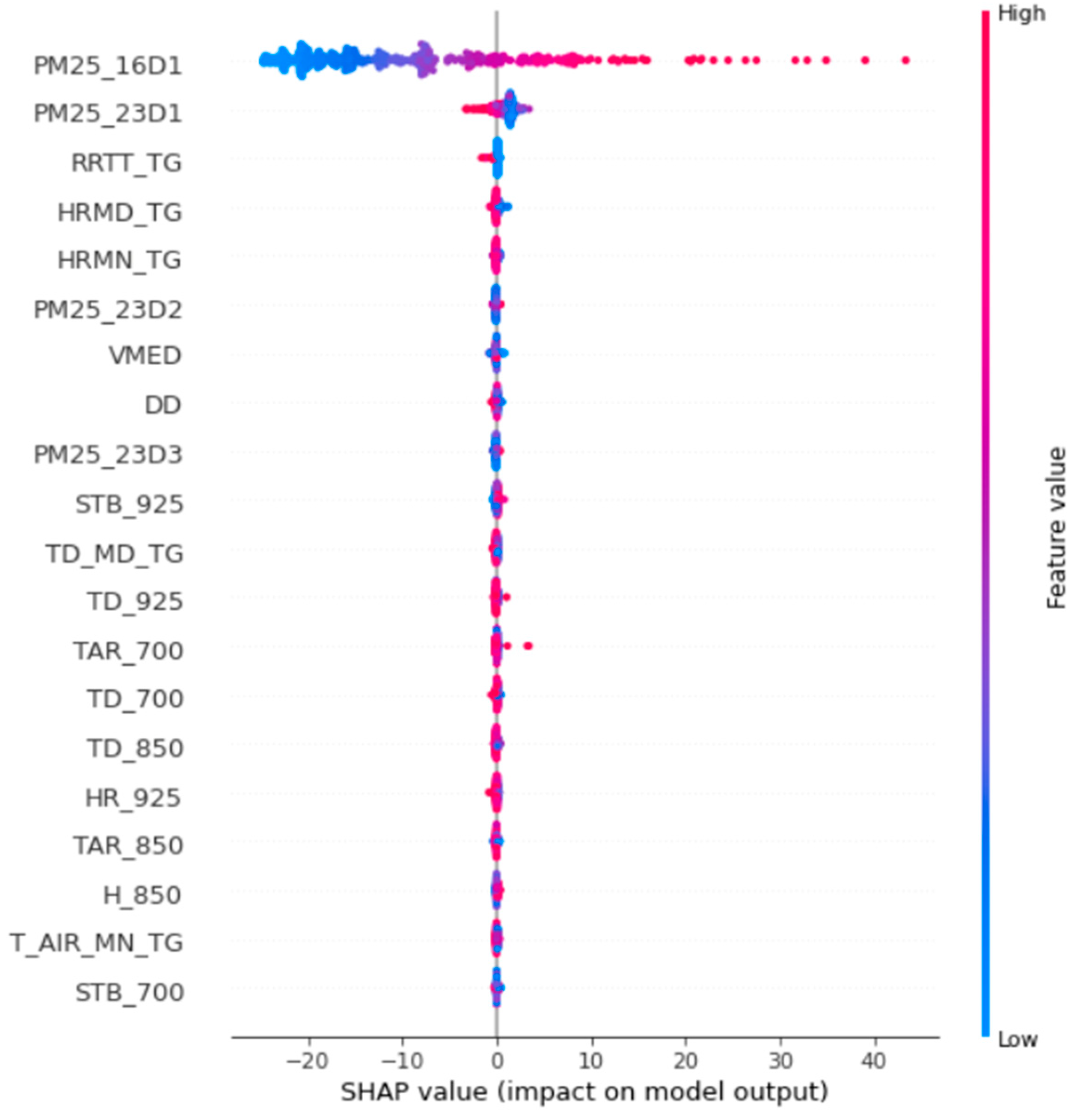
3.3. Feature Selection

Feature selection is a dimensionality reduction technique that can select a small subset of relevant features from the original set by removing noisy, irrelevant, and redundant features, thereby reducing computing time, improving learning accuracy, and enabling a better understanding of the data [27,28]. In this study, Shapley additive explanation (SHAP) values were used to interpret the contribution of features in prediction models. SHAP calculates the impact of each feature on the predictions made by a model. It expresses model predictions as linear combinations of binary variables that describe whether each covariate is present in the model [29,30]. Here, feature selection based on SHAP values was used to create feature-reduced forecast models, and their performances were compared to full-featured counterparts. The SHAP graphs show that the four variables with the highest feature values were selected and applied using machine learning and statistical methods. The model performance indicators with and without feature selection were compared, and only the best results are listed in

Table 2. Comparison of the MLR, RF, GB, and SVR models trained using 2013–2018 data and tested on 2019 data.

Method	Pollutant	Model Performance Indicator				Model Built Using SHAP/Feature Selection
		R2	RMSE	MAE	BIAS	Yes	No
MLR	PM10	0.90	7.14	4.60	0.81		✓
	PM2.5	0.89	4.26	2.84	0.57		✓
RF	PM10	0.89	7.49	4.73	1.01		✓
	PM2.5	0.88	4.56	3.00	0.67	✓
GB	PM10	0.89	7.47	4.73	0.80	✓
	PM2.5	0.88	4.47	2.95	0.77		✓
SVR	PM10	0.89	7.65	4.70	0.16	✓
	PM2.5	0.88	4.57	2.92	0.04	✓

The best results are shown in bold.

,

Table 3. Comparison of the MLR, RF, GB, and SVR models trained using 2013–2018 data and tested on 2020 data.

Method	Pollutant	Model Performance Indicator				Model Built Using SHAP/Feature Selection
		R2	RMSE	MAE	BIAS	Yes	No
MLR	PM10	0.81	10.74	7.83	6.12		✓
	PM2.5	0.61	7.67	5.52	2.91		✓
RF	PM10	0.90	8.15	6.64	5.02		✓
	PM2.5	0.65	6.89	4.78	1.59		✓
GB	PM10	0.85	10.59	8.54	7.11		✓
	PM2.5	0.66	7.43	5.71	3.72		✓
SVR	PM10	0.68	16.13	13.01	11.18	✓
	PM2.5	0.57	11.11	9.24	8.06	✓

The best results are shown in bold.

and

Table 4. Comparison of the MLR, RF, GB, and SVR models trained using 2013–2018 data and tested on 2021 data.

Method	Pollutant	Model Performance Indicator				Model Built Using SHAP/Feature Selection
		R2	RMSE	MAE	BIAS	Yes	No
MLR	PM10	0.90	7.90	6.08	4.16		✓
	PM2.5	0.88	3.92	2.97	1.65		✓
RF	PM10	0.89	8.05	6.14	3.84		✓
	PM2.5	0.89	3.72	2.74	1.47		✓
GB	PM10	0.89	8.98	7.32	5.30		✓
	PM2.5	0.88	4.60	3.85	2.96		✓
SVR	PM10	0.86	13.96	11.92	11.30	✓
	PM2.5	0.79	8.87	7.58	7.40	✓

The best results are shown in bold.

.

3.4. Performance Measures

The machine learning models were built in JupyterLab 3.2.1, using Python 3 and the scikit-learn library. Table 1 shows the variables considered as predictors in the training dataset for the machine learning and statistical models in the air quality forecast in Macao. Model performance indicators, including R² calculated by Equation (1), RMSE calculated by Equation (2), MAE calculated by Equation (3), and systematic error (BIAS) calculated by Equation (4), were used to evaluate the performance of the air quality forecast models with the testing dataset. The equations are defined as

$${\mathrm{R}}^2=\frac{[{\int }_{i=1}^n(f_i-\overline{f} )-\left(o_i-\overline{o} \right){]}^2}{[{\int }_{i=1}^n{(f_{i- }\overline{f})}^2] [{\int }_{i=1}^n{\left(o_i-\overline{o} \right)}^2]}.$$

(1)

$$\mathrm{RMSE}=\sqrt{\frac{1}{n} {\sum }_{i=1}^n{\left(f_i-o_i\right)}^2}$$

(2)

$$\mathrm{MAE}=\frac{1}{n} {\sum }_{i=1}^n\left|f_i-o_i\right|$$

(3)

$$\mathrm{BIAS}=\frac{1}{n} {\sum }_{i=1}^n\left(f_i-o_i\right)$$

(4)

where $f_i$ is the forecast value of the sample i, $\overline{f}$ is the forecast average, $o_i$ is the observation of the sample i, $\overline{o}$ is the observation average, and the n is the number of samples.

4. Results and Discussion

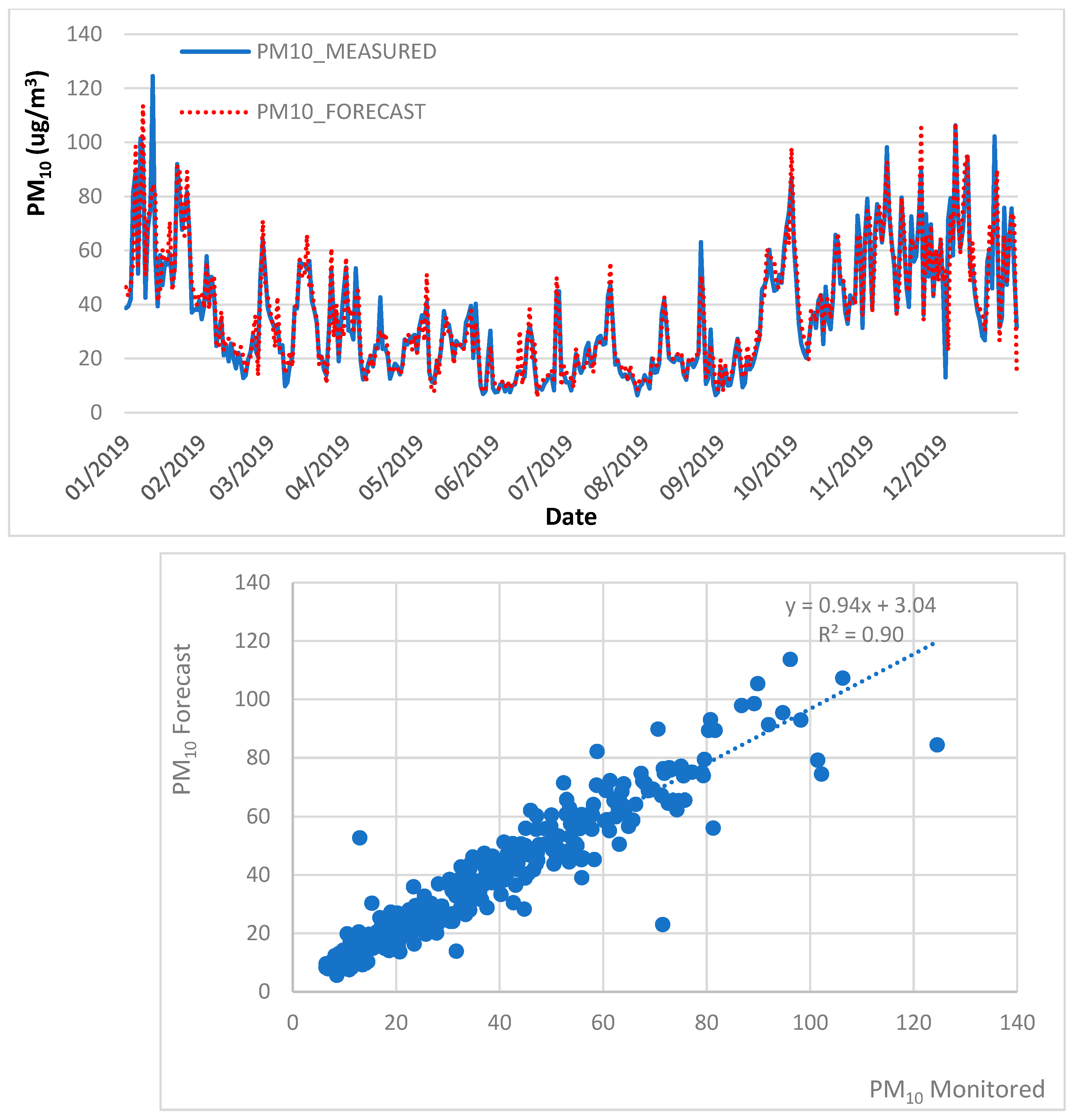
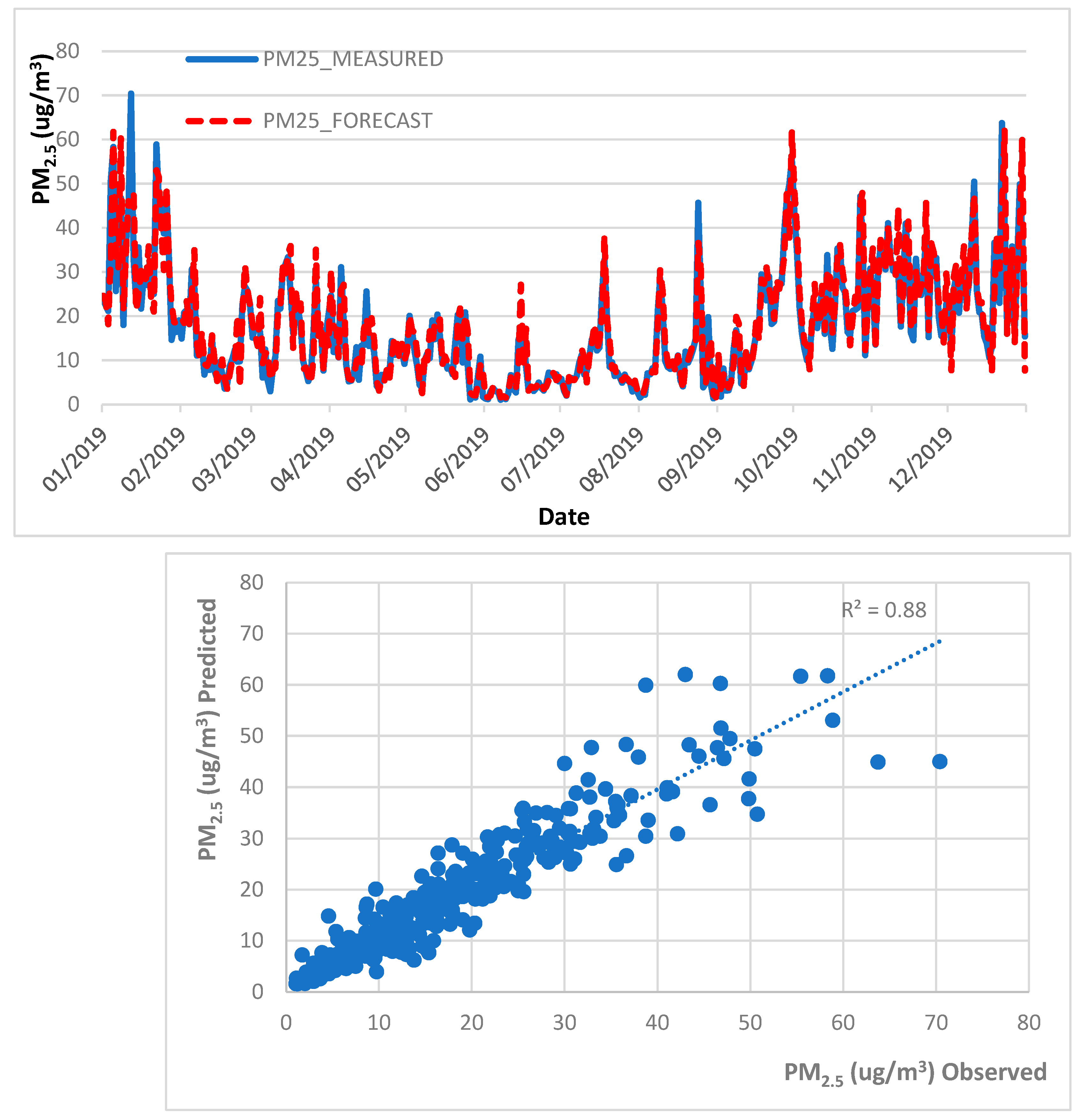
4.1. Air Quality Forecast, 2013–2018 Trained Data, 2019 Test Data

The results of the model performance indicator are listed in Table 2, which shows that MLR without feature selection performed the best in the prediction of PM₁₀ and PM_2.5 amongst different machine learning models with 2013 to 2018 trained data, and validated with 2019 test data. Nevertheless, there is no significant difference amongst MLR, RF, GB, and SVR, with high R² recorded between the predicted and observed data (between 0.88 and 0.90), low RMSE (between 4.26 and 7.65), low MAE (between 2.84 and 4.73), and low BIAS (0.04 to 1.01). The reduced-feature models based on SHAP values do not necessarily yield better results.

Figure 1 shows the observed and predicted PM₁₀ concentrations using MLR in 2019, which offers a high R² of 0.90, the best result out of all the models, and the use of reduced-feature models based on SHAP values was not applied. Figure 1 shows that it is very challenging to predict some of the extremely high-pollution episodes, and the outliers refer to the high concentration, which is challenging to predict by the respective method.

Figure 2 shows the observed and predicted PM_2.5 concentrations using RF in 2019, which offers a high R² of 0.88, a very promising result in the air quality prediction. Figure 2 shows that it is very challenging to predict some of the extremely high pollution episodes, and the outliers refer to the high concentration, which is challenging to predict by the respective method.

Figure 3 shows the SHAP values in the RF model using the 2013 to 2018 trained data and the 2019 test data, which shows the importance and the weighting of each variable of the forecast models. It indicates that PM25_16D1 and PM25_23D1 were the most critical variables in the forecast model as they obtained the highest SHAP values in Figure 3. This result was expected as the pollutant concentrations of previous days had a significant influence on the next day’s forecast.

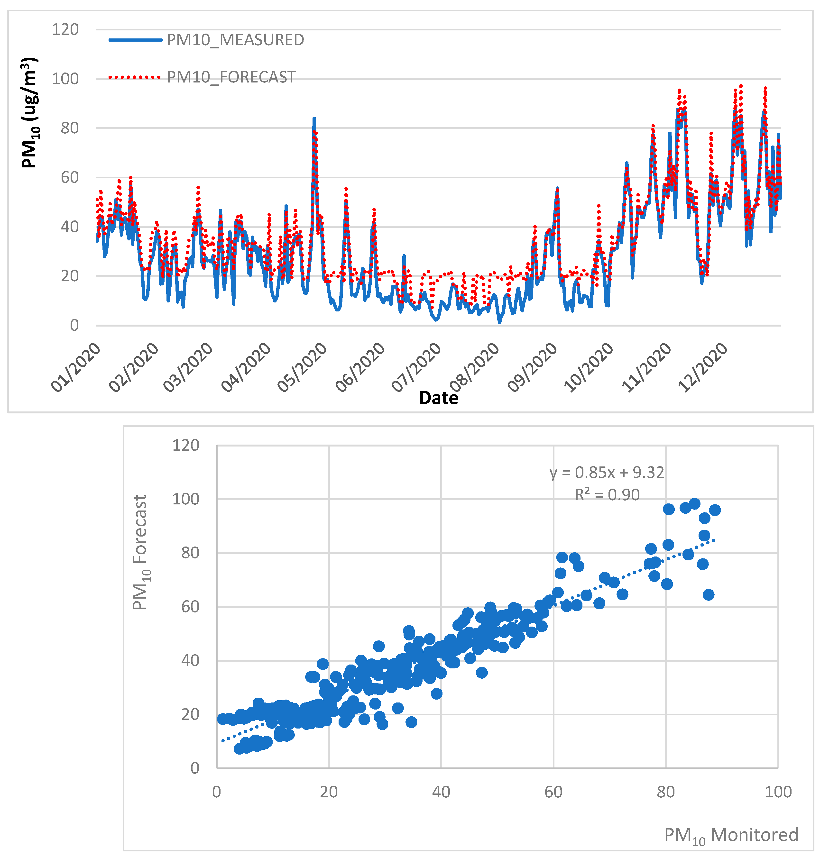
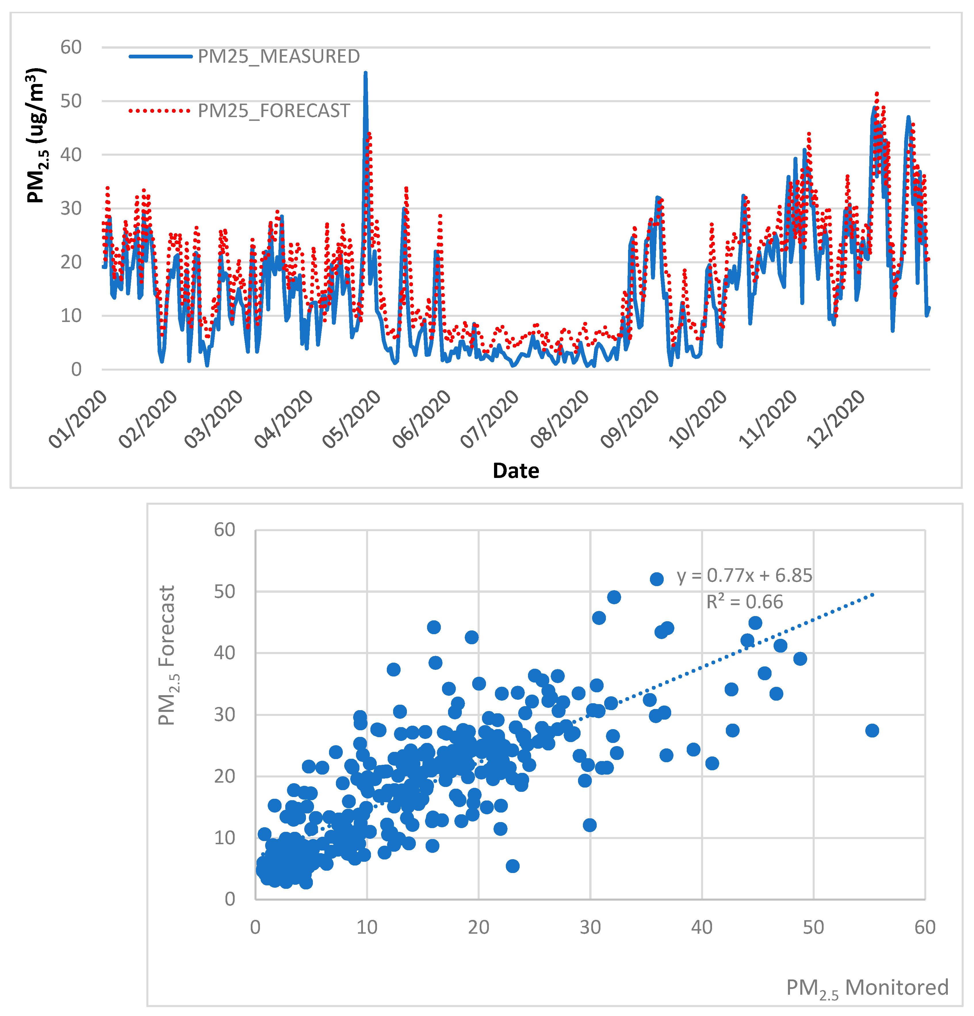
4.2. Air Quality Forecast, 2013 to 2018 Trained Data, 2020 Test Data

The results of the model performance indicators are listed in Table 3, which shows that RF without the use of SHAP values performed the best in the prediction of PM₁₀, and GB without the use of SHAP values performed the best in the prediction of PM_2.5 in the 2013 to 2018 trained data, validated with 2020 test data. Nevertheless, there is a more significant variation in the R² in the 2013 to 2018 trained data validated with 2020 test data (R² between 0.57 and 0.90), high RMSE (between 7.43 and 16.13), high MAE (between 4.78 and 13.01), and high BIAS (between 1.59 and 11.18) in comparison to 2019 test data (with R² from 0.88 to 0.90, RMSE from 4.26 to 7.47, MAE from 2.84 to 4.73, and BIAS from 0.04 to 1.01). This may be attributed to the unusually low levels of PM₁₀ and PM_2.5 concentrations in the second half of 2020 due to the outbreak of the COVID-19 pandemic, which affected the performance of the air quality forecast models. SVR struggled the most to predict the levels of PM_2.5 concentrations in 2020, with an unusual low R² of 0.57. In contrast, MLR, RF, and GB did relatively well in the prediction of PM₁₀ (R² of 0.81, 0.90, and 0.85, respectively) and the prediction of PM_2.5 (R² of 0.61, 0.65, and 0.66, respectively) in the air quality forecast of 2020. The reduced-feature models based on SHAP did not yield better results.

Figure 4 shows observed and predicted PM₁₀ concentrations using RF in 2020, with a high R² of 0.90, the same results as 2019 and 2021. The outbreak of the COVID-19 pandemic did not influence the performance of the PM₁₀ prediction in 2020, which showed the robustness of RF compared to other methods (MLR, GB, and SVR). The use of reduced-feature models based on SHAP values was not applied. Figure 4 shows that it is very challenging to predict some of the extremely low- and high-pollution episodes during the pandemic, and the outliers refer to the low and high concentration, which is challenging to predict by the respective method.

Figure 5 shows observed and predicted PM_2.5 concentrations using GB in 2020, with a moderate R² of 0.66, which tends to overestimate the peaks and misses most of the low-pollution episodes. This may be due to the unusually low levels of PM_2.5 concentration in 2020 compared to the previous years, which falls out of the prediction range for the machine learning and statistical models. Figure 5 shows that it is very challenging to predict some of the extremely low- and high-pollution episodes during the pandemic, and the outliers refer to the low and high concentration, which is challenging to predict by the respective method.

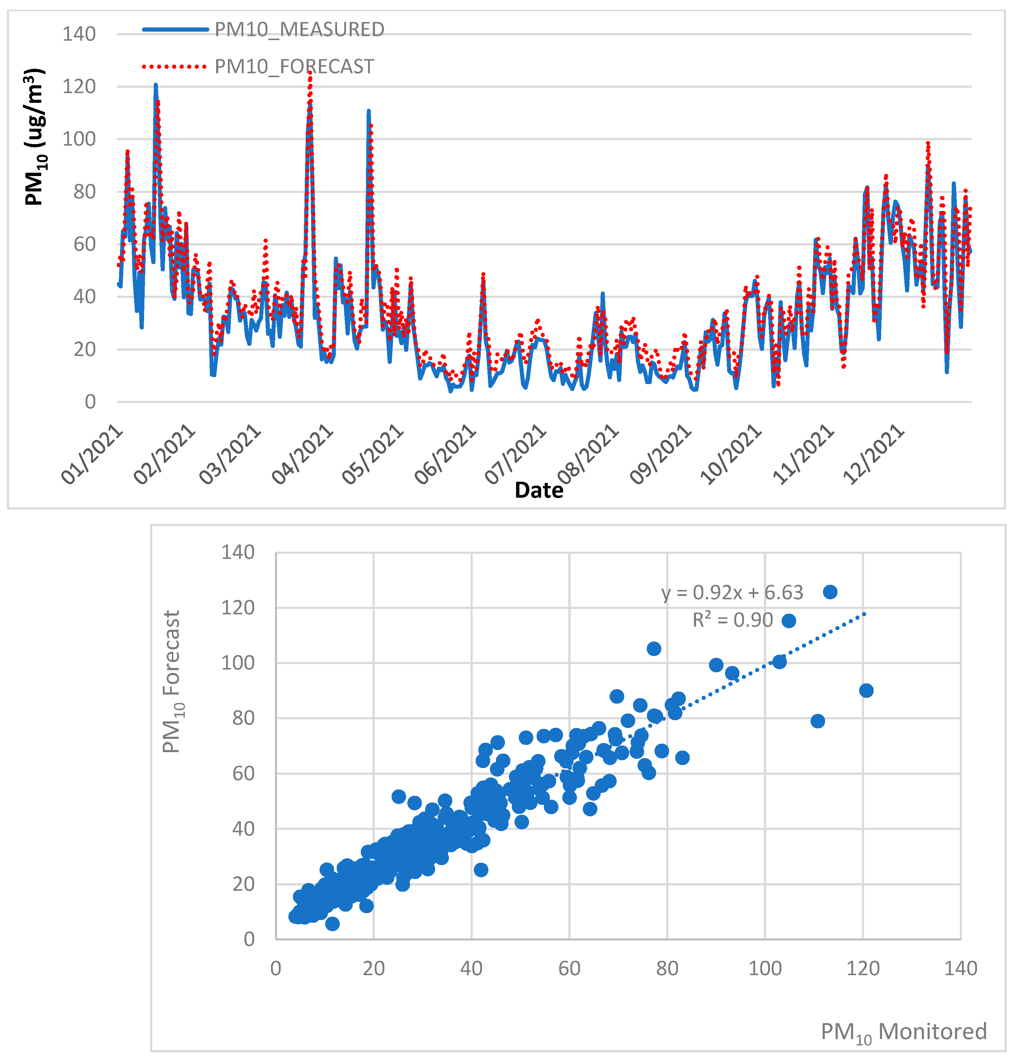
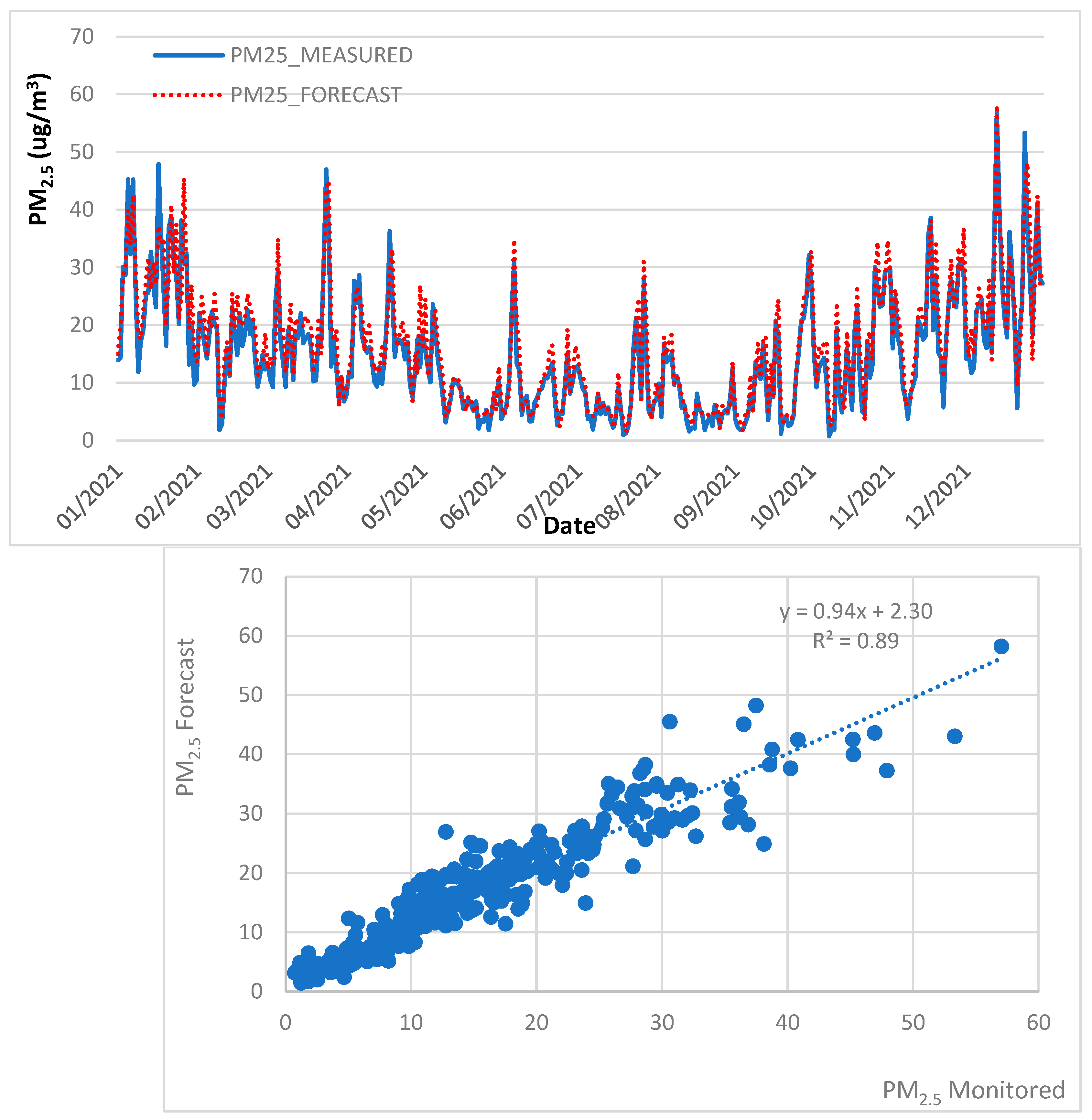
4.3. Air Quality Forecast, 2013 to 2018 Trained data, 2021 Test Data

The results of the model performance indicators are listed in Table 4, which shows that MLR without feature selection performed the best in the prediction of PM₁₀, and RF without feature selection served the best in the prediction of PM_2.5 amongst different machine learning and statistical methods in 2013 to 2018 trained data, validated with 2021 test data. The obtained result of MLR, RF, GB, and SVR in 2019 (R² between 0.88 and 0.90) shows similar results to 2021 (R² between 0.79 and 0.90), with low RMSE (between 3.72 and 13.96), low MAE (between 2.74 and 11.92), and low BIAS (between 1.47 and 11.30). Therefore, there is no significant difference between MLR, RF, and GB, with a high R² recorded between the predicted and observed data (between 0.88 and 0.90), while SVR performed the worst in the prediction of PM_2.5 (with an R² of 0.79). The reduced-feature models based on SHAP do not necessarily yield better results.

Figure 6 shows observed and predicted PM₁₀ concentration using MLR in 2021, with a high R² of 0.90, maintaining a similar level in 2019 and 2020. The use of reduced-feature models based on SHAP values was not applied. Figure 6 shows that it is very challenging to predict some of the extremely high-pollution episodes during the new normal period, and the outliers refer to the high concentration, which is challenging to predict by the respective method.

Figure 7 shows observed and predicted PM_2.5 concentrations using RF in 2021, with a high R² of 0.89, showing that the performance of the PM_2.5 prediction was restored to 2019 levels. The use of reduced-feature models based on SHAP values was not applied. Figure 7 shows that it is very challenging to predict some of the extremely high pollution episodes during the new normal period, and the outliers refer to the high concentration, which is challenging to predict by the respective method.

5. Conclusions

The application of machine learning and statistical methods to forecast the daily average concentration of PM₁₀ and PM_2.5 for the next day, from 2019 to 2021 in the region of Macau, was successful in the Taipa Ambient Air Quality Monitoring Station. The results show that it was more challenging to forecast the levels of PM_2.5 concentration in 2020, as suggested by a lower R² and higher RMSE, MAE, and BIAS, than the PM₁₀ concentration. The levels of PM_2.5 concentration during the outbreak of the COVID-19 pandemic reached a record low, which falls outside of the detection range of the machine learning and statistical methods, thus making it very difficult to make an accurate prediction of the levels of PM_2.5 concentration. Due to the significant decrease in the emission of PM₁₀ and PM_2.5 in the Greater Bay Area (GBA) region, the difficulty of accurately predicting air quality increased substantially. In addition, the variables PM10_16D1, PM10_23D1, PM25_16D1, and PM25_23D1, representing pollutant concentration persistence, played an essential role in predicting PM₁₀ and PM_2.5 for the following days. Nevertheless, the levels of PM₁₀ and PM_2.5 concentration in Macao slowly returned to normal in 2021 as the world adapted to a new normal environment, and the prediction of air quality models in 2021 has been restored to a similar performance before the COVID-19 pandemic in 2019.

References

1. WHO. World Health Statistics 2021: Monitoring Health for the SDGs, Sustainable Development Goals; WHO: Geneva, Switzerland, 2021. [Google Scholar]
2. Zaheer, J.; Jeon, J.; Lee, S.-B.; Kim, J.S. Effect of Particulate Matter on Human Health, Prevention, and Imaging Using PET or SPECT. Prog. Med. Phys. 2018, 29, 81. [Google Scholar] [CrossRef]
3. Dantas, G.; Siciliano, B.; França, B.B.; da Silva, C.M.; Arbilla, G. The impact of COVID-19 partial lockdown on the air quality of the city of Rio de Janeiro, Brazil. Sci. Total Environ. 2020, 729, 139085. [Google Scholar] [CrossRef] [PubMed]
4. Zambrano-Monserrate, M.A.; Ruano, M.A.; Sanchez-Alcalde, L. Indirect effects of COVID-19 on the environment. Sci. Total Environ. 2020, 728, 138813. [Google Scholar] [CrossRef] [PubMed]
5. Fan, K.; Dhammapala, R.; Harrington, K.; Lamastro, R.; Lamb, B.; Lee, Y. Development of a Machine Learning Approach for Local-Scale Ozone Forecasting: Application to Kennewick, WA. Front. Big Data 2022, 5, 781309. [Google Scholar] [CrossRef]
6. Saheer, L.B.; Bhasy, A.; Maktabdar, M.; Zarrin, J. Data-Driven Framework for Understanding and Predicting Air Quality in Urban Areas. Front. Big Data 2022, 5, 822573. [Google Scholar] [CrossRef] [PubMed]
7. Chau, P.N.; Zalakeviciute, R.; Thomas, I.; Rybarczyk, Y. Deep Learning Approach for Assessing Air Quality During COVID-19 Lockdown in Quito. Front. Big Data 2022, 5, 842455. [Google Scholar] [CrossRef]
8. Leong, W.C.; Kelani, R.O.; Ahmad, Z. Prediction of air pollution index (API) using support vector machine (SVM). J. Environ. Chem. Eng. 2020, 8, 103208. [Google Scholar] [CrossRef]
9. Doreswamy; Harishkumar, K.S.; Km, Y.; Gad, I. Forecasting Air Pollution Particulate Matter (PM2.5) Using Machine Learning Regression Models. Procedia Comput. Sci. 2020, 171, 2057–2066. [Google Scholar] [CrossRef]
10. Liang, Y.C.; Maimury, Y.; Chen, A.H.L.; Juarez, J.R.C. Machine learning-based prediction of air quality. Appl. Sci. 2020, 10, 9151. [Google Scholar] [CrossRef]
11. Martínez, N.M.; Montes, L.M.; Mura, I.; Franco, J.F. Machine Learning Techniques for PM 10 Levels Forecast in Bogotá. In Proceedings of the 2018 ICAI Workshops (ICAIW), Bogota, Colombia, 1–3 November 2018. [Google Scholar] [CrossRef]
12. Juarez, E.K.; Petersen, M.R. A Comparison of Machine Learning Methods to Forecast Tropospheric Ozone Levels in Delhi. Atmosphere 2022, 13, 46. [Google Scholar] [CrossRef]
13. Su, Y. Prediction of air quality based on Gradient Boosting Machine Method. In Proceedings of the 2020 International Conference on Big Data and Informatization Education (ICBDIE), Zhangjiajie, China, 23–25 April 2020; pp. 395–397. [Google Scholar] [CrossRef]
14. De Oliveira, R.C.G.; Cunha, C.L.; Tôrres, A.R.; Corrêa, S.M. Forecasts of tropospheric ozone in the Metropolitan Area of Rio de Janeiro based on missing data imputation and multivariate calibration techniques. Environ. Monit. Assess. 2021, 193, 531. [Google Scholar] [CrossRef] [PubMed]
15. Suárez Sánchez, A.; García Nieto, P.J.; Riesgo Fernández, P.; del Coz Díaz, J.J.; Iglesias-Rodríguez, F.J. Application of an SVM-based regression model to the air quality study at local scale in the Avilés urban area (Spain). Math. Comput. Model. 2011, 54, 1453–1466. [Google Scholar] [CrossRef]
16. Lei, M.T.; Monjardino, J.; Mendes, L.; Gonçalves, D.; Ferreira, F. Macao air quality forecast using statistical methods. Air Qual. Atmos. Health 2019, 12, 1049–1057. [Google Scholar] [CrossRef]
17. Lei, M.T.; Monjardino, J.; Mendes, L.; Gonçalves, D.; Ferreira, F. Statistical Forecast of Pollution Episodes in Macao during National Holiday and COVID-19. Int. J. Environ. Res. Public Health 2020, 17, 5124. [Google Scholar] [CrossRef]
18. Mendes, L.; Monjardino, J.; Ferreira, F. Air Quality Forecast by Statistical Methods: Application to Portugal and Macao. Front. Big Data 2022, 5, 826517. [Google Scholar] [CrossRef]
19. Rybarczyk, Y.; Zalakeviciute, R. Machine learning approaches for outdoor air quality modelling: A systematic review. Appl. Sci. 2018, 8, 2570. [Google Scholar] [CrossRef]
20. Liu, H.; Li, Q.; Yu, D.; Gu, Y. Air quality index and air pollutant concentration prediction based on machine learning algorithms. Appl. Sci. 2019, 9, 4069. [Google Scholar] [CrossRef]
21. Ivanov, A.; Voynikova, D.; Stoimenova, M.; Gocheva-Ilieva, S.; Iliev, I. Random forests models of particulate matter PM10: A case study. AIP Conf. Proc. 2018, 2025, 030001. [Google Scholar] [CrossRef]
22. Rybarczyk, Y.; Zalakeviciute, R. Assessing the COVID-19 Impact on Air Quality: A Machine Learning Approach. Geophys. Res. Lett. 2021, 48, e2020GL091202. [Google Scholar] [CrossRef]
23. Lee, M.; Lin, L.; Chen, C.Y.; Tsao, Y.; Yao, T.H.; Fei, M.H.; Fang, S.H. Forecasting Air Quality in Taiwan by Using Machine Learning. Sci. Rep. 2020, 10, 145–154. [Google Scholar] [CrossRef] [PubMed]
24. Liu, B.C.; Binaykia, A.; Chang, P.C.; Tiwari, M.K.; Tsao, C.C. Urban air quality forecasting based on multidimensional collaborative Support Vector Regression (SVR): A case study of Beijing-Tianjin-Shijiazhuang. PLoS ONE 2017, 12, e0179763. [Google Scholar] [CrossRef]
25. Arampongsanuwat, S.; Meesad, P. Prediction of PM 10 using Support Vector Regression. Int. Conf. Inf. Electron. Eng. 2011, 6, 120–124. [Google Scholar]
26. Castelli, M.; Clemente, F.M.; Popovič, A.; Silva, S.; Vanneschi, L. A Machine Learning Approach to Predict Air Quality in California. Complexity 2020, 2020, 8049504. [Google Scholar] [CrossRef]
27. Cai, J.; Luo, J.; Wang, S.; Yang, S. Feature selection in machine learning: A new perspective. Neurocomputing 2018, 300, 70–79. [Google Scholar] [CrossRef]
28. Miao, J.; Niu, L. A Survey on Feature Selection. Procedia Comput. Sci. 2016, 91, 919–926. [Google Scholar] [CrossRef]
29. Futagami, K.; Fukazawa, Y.; Kapoor, N.; Kito, T. Pairwise acquisition prediction with SHAP value interpretation. J. Financ. Data Sci. 2021, 7, 22–44. [Google Scholar] [CrossRef]
30. Gramegna, A.; Giudici, P. SHAP and LIME: An Evaluation of Discriminative Power in Credit Risk. Front. Artif. Intell. 2021, 4, 752558. [Google Scholar] [CrossRef]
Figure 1. Observed and predicted PM10 concentrations using MLR for the year of 2019.
Atmosphere 13 01412 g001
Figure 2. Observed and predicted PM2.5 concentrations using RF for the year 2019.
Atmosphere 13 01412 g002
Figure 3. Feature ranking using the SHAP values for the RF model trained using 2013–2018 data and tested using 2019 data which predicts PM2.5 with SHAP values in 2013 to 2018 trained data and 2019 test data.
Atmosphere 13 01412 g003
Figure 4. Observed and predicted PM10 concentrations using RF for the year 2020.
Atmosphere 13 01412 g004
Figure 5. Observed and predicted PM2.5 concentrations using GB in 2020.
Atmosphere 13 01412 g005
Figure 6. Observed and predicted PM10 concentrations using MLR in 2021.
Atmosphere 13 01412 g006
Figure 7. Observed and predicted PM2.5 concentrations using RF in 2021.
Atmosphere 13 01412 g007