US Clean Energy Futures—Air Quality Benefits of Zero Carbon Energy Policies

Abstract

In this work, we compare the air quality benefits of a variety of future policy scenarios geared towards controlling EGU (electricity generating units) emissions between the present-day conditions and 2050. While these policies are motivated by reducing CO₂ emissions, they also yield significant co-benefits for criteria pollutants, such as ozone and PM_2.5. An integrated set of clean energy policies were examined to assess the time-varying costs and benefits of a range of decarbonization strategies, including business as usual and the Affordable Clean Energy plan, with a primary focus on others that look to achieve very low, if not zero, CO₂ emissions from the EGU sector by 2050. Benefits assessed include mitigation of greenhouse gas emissions as well as air quality co-benefits. In this introductory work, we describe the potential air quality changes from various clean air policies, to set the stage for upcoming work looking at health and monetized benefits. Emission changes for key pollutants are forecast using the Integrated Planning Model (IPM), which are then transformed into emission inputs for the Community Multiscale Air Quality Model (CMAQ). For all primary scenarios considered that achieve large greenhouse gas decreases, significant reductions in ozone and PM are realized, mainly in the eastern US, and all policies produce air quality benefits.

1. Introduction

The energy sector in the US is one of the major contributors of harmful criteria pollutants, such as nitrogen oxides (NO_x), sulfur oxides (SO_x), ozone (O₃), and fine particulate matter (PM_2.5) [1,2,3], with many states within the US struggling to achieve National Ambient Air Quality Standards (NAAQS) [4,5,6]. These pollutants have a variety of deleterious health effects [7,8,9]. With regard to health impacts and achieving the NAAQS, the two pollutants of greatest concern are PM_2.5 and O₃. At the regional scale, both pollutants are largely secondary in nature, being formed in the atmosphere, e.g., by reactions of volatile organic compounds (VOCs) and NO_x for both PM_2.5 and O₃, while SO_x and NH₃ emissions also contribute to PM_2.5 [10,11,12,13]. Primary emissions, e.g., from wildfires and windblown dust, also contribute to PM. Given the recent global push for reductions in greenhouse gas (GHG) emissions, there have been calls for a 100% carbon-free power sector by 2035, with an interim target of 80% clean electricity by 2030, which is consistent with the previously proposed Clean Air Payment Program and somewhat greater than the 2030 reduction expected under the recently passed Inflation Reduction Act (IRA) [14]. Coupled with the increased electrification of both the transportation and building sectors, such a transition could enable the US to comply with the greenhouse gas reduction targets under the Paris Agreement [15,16,17]. Reductions in GHG emissions almost always have resulted in co-benefits, since a shift away from fossil fuel sources typically leads to corresponding decreases in criteria pollutants [18,19,20], particularly O₃ and PM_2.5. Such decreases are important to help local air quality managers meet the NAAQS as regions across the US continue to exceed those standards, particularly for O₃ and PM_2.5. Currently, the O₃ standard, as set by the US EPA, is 70 ppb, defined as the fourth-highest daily maximum 8 h concentration averaged across three consecutive years, while the primary standard for PM_2.5 is set at an annual average of 12 μg m⁻³ [6,21,22,23,24]. Note, both standards are under review [25] and may be tightened, further increasing the importance of strategies that address both GHGs and traditional air pollutants.

The push for a 100% carbon-free power sector by 2035, with 80% clean generation achieved by 2030, has recently been promoted by the Biden Administration. Along with the increased electrification that is taking place in the transportation sector, these policies would allow the United States to attain its 2030 GHG commitment under the Paris Agreement. While there are many ways that such reductions can be achieved, one way is for Congress, through budget reconciliation, to provide financial incentives to “revamp” America’s infrastructure and move towards cleaner forms of energy. The recently passed IRA is an example of such a bill, and it promotes investments in clean energy. However, it is not expected to achieve full compliance with the US Paris commitment. Additional legislation is likely to be needed that could move the country to having 80% of total electricity production by 2030 (80x30) to be from fossil-free sources. This would require heavy investment in renewable energy sources, such as wind and solar, while potentially requiring additional generation from clean energy sources, such as hydroelectric and nuclear. The target for such policies often includes 100% clean energy as early as 2035, and 2050 the latest.

Various policies have been proposed to achieve the above reductions, with a target year of 2050 for net-zero emissions. There has been much focus on Clean Energy Standard (CES) policies, which specify that a percentage of energy needs to be satisfied by clean sources. The definition of clear sources depends on legislative criteria: for example, such sources as natural gas with carbon sequestration and nuclear energy can be deemed clean. Such an approach can be less costly than a more restrictive policy, such as a renewable portfolio standard (RPS), where a percentage of energy generation is required to be derived from renewable sources, such as solar and wind. The CES policy that has gained much traction is the 80x30 CES. Under the 80x30 CES, the federal government would cover a part of the cost associated with adding new, clean sources in energy generation, while at the same time providing incentives to the private sector to retain and increase its investments in clean energy sources. This scenario has the following characteristics: (a) a target of 100% clean energy generation by 2040, (b) use of banked credits being allowed until 2050, (c) the initial carbon intensity benchmark being set at 0.82 tons MWh⁻¹, and (d) natural gas partial crediting being allowed until 2040, based on the emission rate of each plant. Under the above provisions, the policy attains 80% clean energy by the year 2030.

As part of a broad-scale project assessing the viability of various clean air policies, here we determine their efficacy at reducing O₃ and PM_2.5 by performing a modeling study using the Community Multiscale Air Quality (CMAQ) model to simulate how air quality will respond. We examine an array of policy scenarios targeting emissions reductions from EGUs for the years 2030, 2040, and 2050. Emissions are forecast using the Integrated Planning Model (IPM). This is the first part of an interdisciplinary effort from the clean energy futures team, which includes researchers from the Georgia Institute of Technology, Syracuse University, and Resources for the Future. In particular, results presented here will be used in subsequent papers for cost–benefit and health and ecological damage analyses. The overall scope of the entire study includes analyses of the health and environmental impacts and costs of the scenarios. More details on the larger study can be found at available online: https://cleanenergyfutures.syr.edu (accessed on 16 July 2022).

2. Materials and Methods

A series of policies targeted to reduce GHG emissions was analyzed as part of the overall project, as briefly summarized on

Table 1. List and brief description of scenarios of policy options for decarbonization of the electricity sector used in this study.

Policy Type	Policy Cases	Case name
Reference case	“Business as usual”—No Policy enacted	Base case/BAU
Cap and trade	Net 0 emissions in 2040, offsets allowed but no banking	CAP
	Net 0 emissions in 2040; banking allowed	CAP-B
Clean Energy Standard	100% clean in 2050, low carbon intensity benchmark (0.46 metric tons/MWh), total generation, banking allowed until 2040	CES50-L
	100% clean in 2050, high carbon intensity benchmark (0.82 metric tons/MWh), total generation, banking allowed until 2040	CES50-H
	100% clean in 2040, 0.82 metric tons/MWh, partial crediting, total generation, no banking	CES40
	83% clean by 2030, 100% clean by 2040, 0.82 metric tons/MWh, partial crediting, total generation, banking allowed	CES40B
Carbon Price	Carbon price $25/ton rising at 5% per year	CP-25
	Carbon price $50/ton rising at 5% per year	CP-50
Section 111 rules	Affordable Clean Energy (ACE)—assumed 4.5% HRI for affected units	ACE
	Updated Clean Power Plan—achieves 65% CO2 reduction from 2005 levels by 2035	CPP-20

. The Integrated Planning Model was used to assess how those policies would impact air pollutant emissions, the results of which were used for photochemical air quality modeling with the Community Multiscale Air Quality (CMAQ) model. The output of the CMAQ was a set of air pollution and pollutant deposition fields, as detailed below.

2.1. Clean Air Policy Scenarios Analyzed

As part of a large-scale study examining the costs and benefits (including air quality and health), we simulated the air quality outcomes of an array of various policy scenarios, including some based on clean energy standards, carbon price options, and others based on carbon pricing or national cap-and-trade system options for the years 2030, 2040, and 2050. A comprehensive list of the scenarios, along with a short description, is found in Table 1. A more detailed description of the overall project and the scenarios being studied, along with preliminary health and climate-related analyses, can be found at https://cleanenergyfutures.syr.edu (accessed on 16 July 2022).

Due to its high benefit-to-cost ratios and increased feasibility when compared to the others, we focus on one particular scenario: the Clean Energy Standard 40 Banking (CES40B: the 7th scenario listed in Table 1), which achieves 83% clean energy generation by 2030 with banking allowed and 100% clean by 2040, also called 80x30 CES.

2.2. Emissions

The Integrated Planning Model (IPM) was used to project how emissions of pollutants, including CO₂, NO_x, SO_x, and primary PM_2.5, would respond to each of the above policies. IPM is a proprietary, commercial linear optimization model that includes unit-level representation of the entire EGU sector across the US. For given policy constraints, IPM returns the cost-minimizing pattern of generation, including the energy mix used by each facility in the domain, along with other pertinent parameters, including pollutant emissions, total generating power, and costs. It is widely used both by the US Environmental Protection Agency (EPA), as well as other federal and state agencies.

2.3. Chemical Transport Model

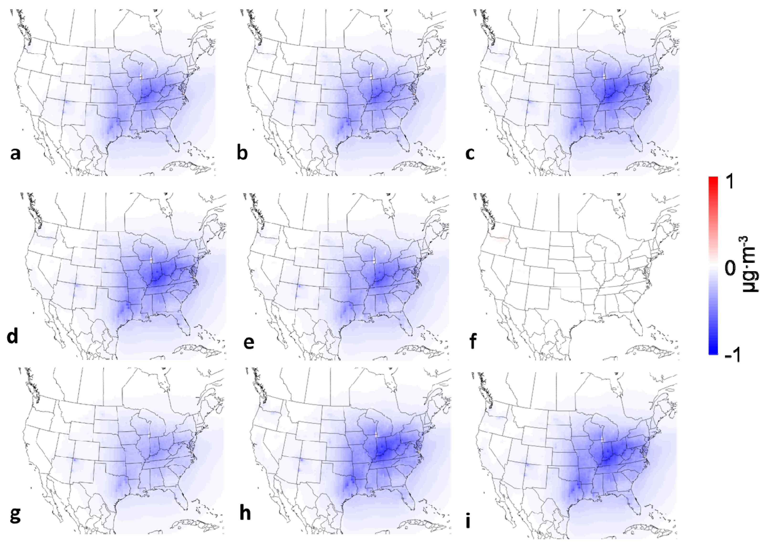
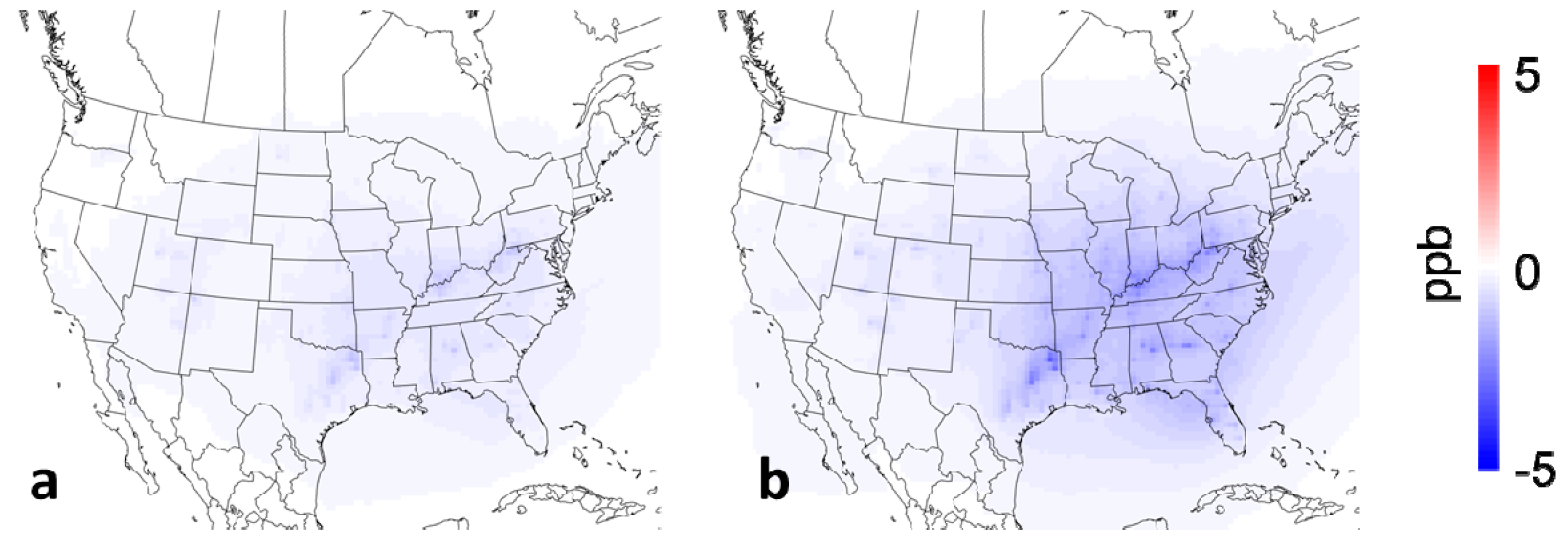
For air quality simulations, we used the CMAQ model [26], a three-dimensional, mass-conserving, chemical transport model that resolves the processing that air quality-pertinent species undergo in the atmosphere, including emissions, chemical reactions, turbulent diffusion, and atmospheric deposition. With regard to the model configuration, CMAQ version 5.0.2 was used with an in-house-developed update described briefly below that allowed for the adjustment of emissions, using ratios derived from IPM results without the need to rerun the emissions preprocessor for each case separately. Simulations were conducted on a 36 × 36 km resolution grid that covered the continental US (CONUS), along with parts of Mexico and Canada. For each scenario, three (3)-year-long simulations were conducted for the years 2030, 2040, and 2050, while one additional simulation for the year 2020 was conducted for the BAU case to serve as a baseline. Input meteorology was generated using the Weather and Research Forecasting (WRF) model. Using future climatology under the Intergovernmental Panel on Climate Change (IPCC) RCP8.5 scenario [27,28], while emissions for the year 2020 were produced using the EPA SMOKE model [29]. The SMOKE-generated emissions were scaled on a state-by-state basis using the IPM output results, in order to determine precursor emissions for each policy scenario and each year. A five (5)-day period served as spin-up for each run in order to initialize the model, while the same methodology was used for all the cases to rule out potential climatological effects on ozone and PM concentrations. For our analysis, daily mean PM_2.5 data were averaged over each year period, while the O₃ data were the seasonal average of the 8 h maximum averages, in accordance with the NAAQS.

3. Results

3.1. Ozone

Figure 1 shows the model-predicted maximum 8 h average ozone concentrations for the years 2020, shown in Figure 1a and 2050 in Figure 1b for the base case (BAU). While modest reductions (<1 ppb) are observed throughout the domain by 2050, particularly in states that were already in nonattainment for ozone, such as Louisiana and California, as they were unable to comply with the federal standard of 70 ppb by 2050.

With regard to the other scenarios, in most cases marked decreases in O₃ are realized by 2050, with sufficient magnitude to drive some non-attainment locations towards attainment (below 70 ppb). Domain-wide reductions/increases on maximum 8-h ozone for all the cases are shown in Figure 2. Of particular note is the Affordable Clean Energy policy which provides no reductions and thus no health benefits. This policy was proposed by the Trump Administration but has been voided by D.C. Circuit Court (US EPA, 2021 (https://www.epa.gov/sites/default/files/2021-02/documents/ace_letter_021121.doc_signed.pdf, accessed on 10 August 2022). All other policies achieve reductions ranging from 3 to 5 ppb, especially across the southern and eastern US, with Texas, Ohio, Indiana, West Virginia, and Pennsylvania reaping the largest benefits. The higher ambition policies (i.e., those with the highest reductions in CO₂ emissions), namely, CAP (Figure 2c), CAP-B (Figure 2d), CES50-H (Figure 2h), and CES50-L (Figure 2i), exhibit the greatest reductions. While some states benefit more than others, the reductions are widespread throughout the eastern US, with all eastern states reaping significant air quality and associated health benefits. Note that the magnitude of reductions is not related to the initial ozone values in 2020 (Figure 1a,b and Figure 2), which indicates that ozone in the states with the smallest improvements is largely driven by the emissions of sectors other than the power sector, such as transportation, oil, and gas. In such cases, additional controls and/or increased electrification of the on-road vehicle fleet could significantly magnify the air quality benefits and associated improved health outcomes.

3.2. PM_2.5

The predicted annual mean PM_2.5 concentrations for the years 2020 (Figure 3a) and 2050 (Figure 3b) are shown in Figure 3 for the base case. Similarly to ozone, concentrations are reduced throughout the domain by 2050, but reductions are not only more uniformly distributed across the US but are also of increased relative magnitude. The larger magnitude is likely due to higher relative reductions of PM_2.5 precursors when compared to ozone, especially SO_x and the corresponding sulfate aerosol that comprises a significant portion of total PM_2.5.

As with ozone, the most ambitious policies tend to be those that yield the highest reductions to particulate matter (Figure 4), of up to 1 μg m⁻³: a more than 8% improvement over the standard. Once again, the Affordable Clean Energy policy does not provide any air quality benefits relative to the BAU case, while the CAP (Figure 4c), CAP-B (Figure 4d), CES50-H (Figure 4h) and CES50-L (Figure 4i) tend to provide the greatest reductions.

Similarly to O₃, not all states are equally impacted by reductions: Texas, Ohio, Indiana, West Virginia, and Pennsylvania are projected to experience large reductions in PM_2.5 concentrations. Due to the complexity of particulate matter formation that encompasses multiple species, both anthropogenic and biogenic, and both directly emitted as well as formed in the atmosphere, it is increasingly difficult to control secondary PM formation when compared to O₃ (which responds well to VOC and NO_x controls, depending on the relative abundance of these two precursors). Nevertheless, the observed reductions would be expected to yield significant reductions in pollutant exposures.

A similar pattern is evident in population-weighted exposure (Figure 5). When comparing BAU to other policies, the higher ambition policies result in greater exposure reductions, with the CES50-L policy having the greatest benefits (Figure 5). The ACE rule retains very similar exposure as the BAU both for O₃ and PM_2.5, highlighting the ineffectiveness of the policy at producing benefits. Note that while PM exposure scales almost linearly with CO₂ reductions, the same does not apply for O₃; rather, the Clean Energy Standard policies tend to obtain more significant O₃ exposure improvements for an equivalent reduction in CO₂ emissions when compared to other policies, due to the higher degree of integration of clean energy sources to cover grid needs.

3.3. Clean Energy Standard (CES) CES40B—An 80x30 policy

As discussed in our report “An 80x30 Clean Electricity Standard: Carbon, Costs, and Health Benefits” [30], found at https://cleanenergyfutures.syr.edu (accessed on 16 July 2022)., as well as upcoming publications, the CES40B policy offers air quality improvements similar to the CAP policy at a lower cost (~80% of CAP). Specifically, this policy has a target of 100% clean energy by 2040, with a carbon intensity benchmark of 0.82 metric tons/MWh, that allows partial crediting for natural gas, as well as banking of credits. It reaches 83% clean generation by 2030, with a corresponding 83% reduction in CO₂ emissions from 2005 levels. It yields an estimated $637 billion in climate benefits, with a total cost of enactment of $342 billion, a 13% increase over BAU system costs [30]. When compared to the other policy scenarios evaluated in this study, it provides the highest overall climate benefits, with a cumulative reduction in CO₂ emissions by 30 billion metric tons between 2020 and 2050. In addition, it achieves considerable reduction in air pollution in the form of co-benefits. For ozone, limited reductions are achieved by 2030 (Figure 6a), with most occurring by 2050 (Figure 6b). This pattern is to be expected, since the policy utilizes partial crediting and also increases in stringency over time. Similarly to the previously discussed cases, eastern states, such as Ohio and Pennsylvania, are projected to experience the largest reductions, both in 2030 and 2050.

PM_2.5 reductions tend to be more drastic, with an average of 0.5 μg m⁻³ less PM_2.5 in the eastern US by 2030 (Figure 7b), and up to 1 μg m⁻³ by 2050 (Figure 7b), which is on par with highest-ambition policies. The spatial pattern of reductions is identical to other policies considered (Figure 4).

4. Discussion

In this work, we investigated a variety of energy policies aimed at reducing CO₂ emissions from EGUs and projected the resulting potential air quality co-benefits of those policies. We found that the corresponding improvement in air quality, through reductions in emissions that lead to increases in ozone and PM_2.5 concentrations, can be substantial. With the exception of the BAU and ACE, all of the policies considered generate reductions for both ozone and particulate matter by 2050 to varying extents. Due to the relatively heavy reliance of the eastern US on coal for energy generation, the largest reductions in pollutants after policy implementation are observed over the east, with a maximum decrease of 5 ppb for O₃ and 1 μg m⁻³ for PM_2.5. Such reductions can provide large health benefits and help areas reach attainment of the NAAQS. Our CES40B policy achieves an 80% reduction in CO₂ by 2030 (i.e., 80x30), which has been a proposed target and found to be achievable [31], and would also lead to significant air quality-related benefits by 2030, and those benefits increase in 2040 and 2050. We did not examine potential strategies aimed at reducing CO₂ emissions from non-EGU sectors, most notably the transportation sector. Electrification of mobile sources would lead to reductions in tailpipe emissions of ozone and PM_2.5 precursors, though it would also increase demand on electricity generation. While such policies would increase EGU emissions, the clean air policies examined here would also provide even greater benefits than modeled.

References

1. Holland, D.M.; Principe, P.P.; Sickles, J.E. Trends in atmospheric sulfur and nitrogen species in the eastern United States for 1989–1995. Atmos. Environ. 1999, 33, 37–49. [Google Scholar] [CrossRef]
2. Howarth, R.W.; Boyer, E.W.; Pabich, W.J.; Galloway, J.N. Nitrogen use in the United States from 1961–2000 and potential future trends. Ambio 2002, 31, 88–96. [Google Scholar] [CrossRef] [PubMed]
3. Wilson, J.H.; Mullen, M.A.; Bollman, A.D.; Thesing, K.B.; Salhotra, M.; Divita, F.; Neumann, J.E.; Price, J.C.; DeMocker, J. Emission projections for the US environmental protection agency section 812 second prospective Clean Air Act Cost/benefit analysis. J. Air Waste Manage. Assoc. 2008, 58, 657–672. [Google Scholar] [CrossRef] [PubMed]
4. He, H.; Liang, X.Z.; Sun, C.; Tao, Z.N.; Tong, D.Q. The long-term trend and production sensitivity change in the US ozone pollution from observations and model simulations. Atmos. Chem. Phys. 2020, 20, 3191–3208. [Google Scholar] [CrossRef]
5. Craig, K.; Erdakos, G.; Chang, S.Y.; Baringer, L. Air quality and source apportionment modeling of year 2017 ozone episodes in Albuquerque/Bernalillo County, New Mexico. J. Air Waste Manage. Assoc. 2020, 70, 1101–1120. [Google Scholar] [CrossRef]
6. Jaffe, D.A.; Ninneman, M.; Chan, H.C. NOx and O3 Trends at US Non-Attainment Areas for 1995–2020: Influence of COVID-19 Reductions and Wildland Fires on Policy-Relevant Concentrations. J. Geophys. Res.-Atmos. 2022, 127, 14. [Google Scholar] [CrossRef]
7. Casey, J.A.; Su, J.S.G.; Henneman, L.R.F.; Zigler, C.; Neophytou, A.M.; Catalano, R.; Gondalia, R.; Chen, Y.T.; Kaye, L.; Moyer, S.S.; et al. Improved asthma outcomes observed in the vicinity of coal power plant retirement, retrofit and conversion to natural gas. Nat. Energy 2020, 5, 398–408. [Google Scholar] [CrossRef]
8. Gauderman, W.J.; Urman, R.; Avol, E.; Berhane, K.; McConnell, R.; Rappaport, E.; Chang, R.; Lurmann, F.; Gilliland, F. Association of Improved Air Quality with Lung Development in Children. N. Engl. J. Med. 2015, 372, 905–913. [Google Scholar] [CrossRef]
9. Chestnut, L.G.; Mills, D.M. A fresh look at the benefits and costs of the US Acid Rain Program. J. Environ. Manage. 2005, 77, 252–266. [Google Scholar] [CrossRef]
10. Simon, H.; Reff, A.; Wells, B.; Xing, J.; Frank, N. Ozone Trends Across the United States over a Period of Decreasing NOx and VOC Emissions. Environ. Sci. Technol. 2015, 49, 186–195. [Google Scholar] [CrossRef] [Green Version]
11. Pusede, S.E.; Cohen, R.C. On the observed response of ozone to NOx and VOC reactivity reductions in San Joaquin Valley California 1995-present. Atmos. Chem. Phys. 2012, 12, 8323–8339. [Google Scholar] [CrossRef]
12. Zaveri, R.A.; Berkowitz, C.M.; Kleinman, L.I.; Springston, S.R.; Doskey, P.V.; Lonneman, W.A.; Spicer, C.W. Ozone production efficiency and NOx depletion in an urban plume: Interpretation of field observations and implications for evaluating O3-NOx-VOC sensitivity. J. Geophys. Res.-Atmos. 2003, 108, 23. [Google Scholar] [CrossRef]
13. Atkinson, R. Atmospheric chemistry of VOCs and NOx. Atmos. Environ. 2000, 34, 2063–2101. [Google Scholar] [CrossRef]
14. Rennert, K.; Roy, N.; Burtraw, D. Modeled Effects of Inflation Reduction Act of 2022; Resources for the Future: Washington, DC, USA, 2022. [Google Scholar]
15. Saelen, H.; Hovi, J.; Sprinz, D.; Underdal, A. How US withdrawal might influence cooperation under the Paris climate agreement. Environ. Sci. Policy 2020, 108, 121–132. [Google Scholar] [CrossRef]
16. Pickering, J.; McGee, J.S.; Stephens, T.; Karlsson-Vinkhuyzen, S.I. The impact of the US retreat from the Paris Agreement: Kyoto revisited? Clim. Policy 2018, 18, 818–827. [Google Scholar] [CrossRef]
17. Nong, D.; Siriwardana, M. Effects on the US economy of its proposed withdrawal from the Paris Agreement: A quantitative assessment. Energy 2018, 159, 621–629. [Google Scholar] [CrossRef]
18. Liu, J.Y.; Woodward, R.T.; Zhang, Y.J. Has Carbon Emissions Trading Reduced PM2.5 in China? Environ. Sci. Technol. 2021, 55, 6631–6643. [Google Scholar] [CrossRef]
19. Yang, H.; Pham, A.T.; Landry, J.R.; Blumsack, S.A.; Peng, W. Emissions and Health Implications of Pennsylvania’s Entry into the Regional Greenhouse Gas Initiative. Environ. Sci. Technol. 2021, 55, 12153–12161. [Google Scholar] [CrossRef]
20. Vandepaer, L.; Panos, E.; Bauer, C.; Amor, B. Energy System Pathways with Low Environmental Impacts and Limited Costs: Minimizing Climate Change Impacts Produces Environmental Cobenefits and Challenges in Toxicity and Metal Depletion Categories. Environ. Sci. Technol. 2020, 54, 5081–5092. [Google Scholar] [CrossRef]
21. David, L.M.; Ravishankara, A.R.; Brey, S.J.; Fischer, E.V.; Volckens, J.; Kreidenweis, S. Could the exception become the rule? ‘Uncontrollable’ air pollution events in the US due to wildland fires. Environ. Res. Lett. 2021, 16, 8. [Google Scholar] [CrossRef]
22. Zhang, H.; Srinivasan, R. A Systematic Review of Air Quality Sensors, Guidelines, and Measurement Studies for Indoor Air Quality Management. Sustainability 2020, 12, 9045. [Google Scholar] [CrossRef]
23. DeWitt, H.L.; Crow, W.L.; Flowers, B. Performance evaluation of ozone and particulate matter sensors. J. Air Waste Manage. Assoc. 2020, 70, 292–306. [Google Scholar] [CrossRef] [PubMed]
24. Collet, S.; Kidokoro, T.; Karamchandani, P.; Jung, J.; Shah, T. Future year ozone source attribution modeling study using CMAQ-ISAM. J. Air Waste Manage. Assoc. 2018, 68, 1239–1247. [Google Scholar] [CrossRef]
25. Clean Air Scientific Advisory Committee (CASAC). Available online: https://casac.epa.gov/ords/sab/f?p=113:1: (accessed on 10 August 2022).
26. Byun, D.; Schere, K.L. Review of the governing equations, computational algorithms, and other components of the models-3 Community Multiscale Air Quality (CMAQ) modeling system. Appl. Mech. Rev. 2006, 59, 51–77. [Google Scholar] [CrossRef]
27. Riahi, K.; Rao, S.; Krey, V.; Cho, C.H.; Chirkov, V.; Fischer, G.; Kindermann, G.; Nakicenovic, N.; Rafaj, P. RCP 8.5-A scenario of comparatively high greenhouse gas emissions. Clim. Change 2011, 109, 33–57. [Google Scholar] [CrossRef]
28. Meinshausen, M.; Smith, S.J.; Calvin, K.; Daniel, J.S.; Kainuma, M.L.T.; Lamarque, J.F.; Matsumoto, K.; Montzka, S.A.; Raper, S.C.B.; Riahi, K.; et al. The RCP greenhouse gas concentrations and their extensions from 1765 to 2300. Clim. Change 2011, 109, 213–241. [Google Scholar] [CrossRef]
29. Dennis, R.L.; Byun, D.W.; Novak, J.H.; Galluppi, K.J.; Coats, C.J.; Vouk, M.A. The next generation of integrated air quality modeling: EPA’s Models-3. Atmos. Environ. 1996, 30, 1925–1938. [Google Scholar] [CrossRef]
30. Driscoll, C.; Lambert, K.F.; Wilcoxen, P.; Russell, A.; Burtraw, D.; Domeshek, M.; Mehdi, Q.; Shen, H.; Vasilakos, P. An 80x30 Clean Electricity Standard: Carbon, Costs, and Health Benefits. Available online: https://cleanenergyfutures.syr.edu/wp-content/uploads/2021/07/CEF-80x30-CES-Report_Final_July_9_21.pdf (accessed on 16 July 2022).
31. Esposito, D. Studies Agree 80 Percent Clean Electricity By 2030 Would Save Lives and Create Jobs at Minimal Cost; Energy Innovation: San Franscisco, CA, USA, 2021. [Google Scholar]
Figure 1. Average of seasonal maximum 8-hour ozone average concentrations across the domain for the Business as Usual (BAU), (a) for 2020 and (b) 2050 in ppb. California and Louisiana shown on the map.
Atmosphere 13 01401 g001
Figure 2. Differences in the seasonal average of the maximum 8 h ozone average concentrations in ppb, across the domain for the year 2050 between BAU and: (a) CP-25u, (b) CP-50u, (c) CAP, (d) CAP-B, (e) CES40, (f) ACE, (g) CPP20, (h) CES50-H and (i) CES50-L.
Atmosphere 13 01401 g002
Figure 3. Mean PM2.5 concentrations across the domain for (a) 2020 and (b) 2050 in μg m−3.
Atmosphere 13 01401 g003
Figure 4. Difference between annual mean PM2.5 concentrations in μg m−3 across the domain for the year 2050 between BAU and: (a) CP-25u, (b) CP-50u, (c) CAP, (d) CAP-B, (e) CES40, (f) ACE, (g) CPP20, (h) CES50-H and (i) CES50-L.
Atmosphere 13 01401 g004
Figure 5. Population-weighted reductions in (a) PM2.5 (in μg m3), and (b) O3 (ppb), between each policy and the BAU case for the year 2050, as a function of CO2 reductions (in million metric tons).
Atmosphere 13 01401 g005
Figure 6. Difference in seasonal average maximum 8 h ozone average concentrations in ppb, across the domain for the year (a) 2030 and (b) 2050 between BAU and CES40B.
Atmosphere 13 01401 g006
Figure 7. Differences in mean PM2.5 concentrations in μg m−3, across the domain for the year (a) 2030 and (b) 2050 between BAU and CES40B.
Atmosphere 13 01401 g007