Elucidating the Chemical Compositions and Source Apportionment of Multi-Size Atmospheric Particulate (PM₁₀, PM_2.5 and PM₁) in 2019–2020 Winter in Xinxiang, North China

Abstract

The pollution characteristics of multi-size atmospheric particulates in Xinxiang, which was one of the most polluted cities across China, are still unclear even through air quality in Xinxiang has been improved in recent years. PM₁₀, PM_2.5, and PM₁ samples were synchronously collected from 21 December 2019 to 17 January 2020 to explore pollution levels and reveal sources of PM in Xinxiang. The average mass concentrations of PM₁₀, PM_2.5, and PM₁ were as high as 155.53 μg m⁻³, 120.07 μg m⁻³, and 85.64 μg m⁻³ during the observation period, respectively. Almost all of the chemical compositions in PM₁₀, PM_2.5 and PM₁ increased continuously and obviously with the aggravation of the pollution level. Compared with the clean period, the enhancement of sulfate (23–27%) in PM was obvious higher than nitrate (19–22%) during the pollution period, which demonstrated that sulfate was the main contributor to the high concentration of PM in this study. Similar source distributions for PM₁₀, PM_2.5, and PM₁ were also found, including traffic source, combustion source, secondary aerosols, industrial source, and fugitive dust, by using the positive matrix factorization (PMF) model. Furthermore, the contributions of the combustion source and secondary aerosol were found to be higher in smaller particles (PM_2.5 and PM₁), while the contribution of fugitive dust was higher in PM₁₀. Moreover, dust and sand were entrained by air masses from the northwest that increased the contribution of dust in PM at the observation site. The potential source contribution function (PSCF) analysis illustrated that regional emission sources in northern and eastern Xinxiang might be important potential contributors to PM pollution in Xinxiang.

1. Introduction

Due to sharply increasing energy consumption, rapid economic development, and urbanization, persistent heavy haze pollution processes featuring high PM concentrations occur frequently in China, especially in North China in recent years, which has gained widespread attention [1,2,3,4]. Fine particulate (PM_2.5, with an aerodynamic diameter smaller than 2.5 μm; Abbreviations were summarized in Table S1) and inhalable particle (PM₁₀, particulate matter with aerodynamic diameter smaller than 10 μm) matter have dominated pollution episodes [5] in winter and attracted extensive attention due to their adverse effects on health [4,6,7], atmospheric quality [8], climate change [9], and visibility degradation [10]. The North China region, which contains the Beijing–Tianjin–Hebei region (BTH) and its surrounding provinces (e.g., Henan, Shanxi, Shandong), has a high population density, and a high presence of motor vehicles, and energy intensive and heavily polluted industries in China. According to the Ministry of Ecology and Environment Protection of China (MEEP), the top ten most polluted cities in China in 2021 were all located in the North China region. Therefore, pollution characteristics, source apportionment, formation mechanism, and risk assessment of PM_2.5 and PM₁₀ were conducted over the past several years [4,11,12,13,14,15]. Submicron aerosols (PM₁, particulate matter with an aerodynamic diameter of smaller than 1 μm), as the smaller diameter airborne particles, played more important roles on haze formation, exposure risk, and climate change. However, studies on pollution level, source, and the transport pattern of PM₁ as well as distributions characteristics of chemical species in multi-size airborne particles (PM₁₀, PM_2.5 and PM₁) in North China are scarce.

Multiple studies have been conducted covering the characteristics of PM₁ in some cities based on online continuous observation. Wang et al. [16] studied the non–refractory submicron aerosol (NR–PM₁) in 2016 winter in Beijing and explored fast aqueous–phase transformation of primary organic aerosol (POA) emitted by fossil combustion to secondary organic aerosol (SOA) by an aerodyne SP–AMS. Non fossil sources were an important contributor to SOA in NR–PM₁ as reported by Zhang et al. [17]. The characteristics and source of organic aerosol in NR–PM₁ at high altitudes (260 m) were clarified by Zhou et al. [18]. Similar findings were also found in Atlanta, that is OA dominated NR–PM₁ in all seasons, reported by Rattanavaraha et al. (2017) [19]. Such measurements based on online equipment provide high temporal resolution observation data [20,21], but the species covered were organic matter, nitrate, ammonium, sulfate, and chloride, while the variation of other crucial compositions (e.g., element carbon and heavy metals) was not exhibited. Further studies on the source identification of PM₁ as well as the distribution patterns of chemical species in various size particles are limited. Furthermore, the pollution evolution in multi–size airborne particles during heavy pollution episodes in winter is also lacking.

Xinxiang, a medium–sized industrial city, is located in the northern area of Henan province. It is situated on the North China Plain and is adjacent to Taihang Mountain on the west, with a population of 6.3 million in 2020 (Henan Statistical Yearbook, 2021), covering an area of 8249 km². Xinxiang has experienced serious atmospheric pollution, which was characterized by high PM concentration in recent years [2,22]. Fossil fuel and bio-fuel combustion, motor vehicles, fugitive dust and industrial process were identified as major contributors to PM pollution [2,22,23]. Research on the pollution pattern of multi-size particles and their source identification in Xinxiang is not available as far as we are aware.

Based on the results of previous studies, in this work, multi-size atmospheric particulate (PM₁₀, PM_2.5 and PM₁) were simultaneously collected during the winter of 2019–2020. Their chemical species, including organic carbon (OC), element carbon (EC), water soluble ions and elements were determined. The primary research aimed to explore the following: (1) demonstrate the variation patterns of chemical species in PM₁₀, PM_2.5, and PM₁ during observation periods; (2) explore the evolution and driving force of different pollution episodes; (3) reveal the major contribution sources and explore the region-transport influences of multi-size atmospheric particles.

2. Data and Methodology

2.1. Description of Station and Airborne Particles Sampling

Multi-size airborne particles (PM₁₀, PM_2.5 and PM₁) sampling was simultaneously conducted from 21 December 2019 to 17 January 2020 on the roof of the South Building of Chemistry in Henan Normal University (113.91° E, 35.33° N, 72 m a.s.l) at a height of approximately 20 m from the ground (Figure 1). The location of the sampling site was surrounded by residential zones, commercial areas, and without a nearby industrial source, which represented a typical urban site in the central zone of Xinxiang. Xinxiang is a typical industrial city, and the consumption of coal and nitrogenous fertilizer, pollutants and other characteristics are summarized in Table S2. The samples of PM were simultaneously collected on 90 mm quartz membrane filters (Pallflex Tissuquartz^TM, Pall Corporation, Port Washington, NY, USA) every day from 9:00 a.m. to 8:00 a.m. of the next day (23 h) using TH–150F medium volume air particulate matter samplers (Wuhan Tianhong Instruments Co., Ltd., Wuhan, China) at a flow rate of 100 L min⁻¹, according to the sampling methodology of previous studies [2,24] and technical specification (HJ 656–2013). During the entire sampling campaign, a total of 82 effective samples loaded with PM were obtained (28, 27 and 27 samples were collected for PM₁₀, PM_2.5 and PM₁, respectively). In addition, six field blanks at each site were analyzed in the same way to evaluate the background value. Strict quality assurance and quality control (QA/QC) procedures were performed to ensure the collection of reliable data.

2.2. Sample Analysis

All the quartz filters, which were packaged with tin paper, were baked at 450 °C for 4 h in a muffle furnace to remove organic components prior to sampling [2]. After sampling, the aerosol-loads filters with PM were individually placed in Petri slides in the dark and stored at –20 °C prior to weighing and their subsequent analysis to prevent the evaporation of volatile components [25]. Before and after sampling, all filters were conditioned under a clean room under controlled conditions (constant temperature: 25 ± 1 °C; relative humidity: 50 ± 2%) for at least 24 h in order to minimize the influence of water adsorption and then weighed by using a microbalance tool (Mettler Toledo, XPE205, Columbus, OH, USA) with a reading precision of ± 10 μg. One quarter of each sample membrane was ultrasonically extracted using 15 mL ultrapure water (with a specific resistivity of 18.2 MΩ cm; Millipore, MA, USA) for 40 min at room temperature (20–25 °C). The extracted solutions were then filtered through a 0.45 μm PTFE (Polytetrafluoroethylene) microporous membrane using syringe filters. Eight of the water-soluble inorganic ions (WSII, including Na⁺, NH₄⁺, K⁺, Mg²⁺, Ca²⁺, Cl⁻, NO₃⁻, and SO₄²⁻) were analyzed by performing ion chromatography (IC, Dionex 600, Sunnyvale, CA, USA). For the analysis of carbonaceous components, a 0.53 cm² fraction from another quarter of each sample was determined by performing the thermal–optical reflectance (TOR) method using a Multi-wavelength Carbon Analyzer (DRI model 2015, Desert Research Institute, Reno, NV, USA) following the Interagency Monitoring of Protected Visual Environments_A (IMPROVE_A) protocol. The microwave digestion system (MARS Xpress, CEM, Matthews, NC, USA) was used to digest the filter samples with an acid mixture (3 mL HF + 5 mL HNO₃) for elemental analysis. Inductively coupled plasma atomic emission spectrometry (ICP–AES, SPECTRO Analytical Instruments GmbH, SPECTRO ACROS EOP, Kleve, Germany) was used to detect 19 trace elements in the digestion solution, including Al, As, Ba, Ca, Cd, Co, Cr, Cu, Fe, K, Mg, Mn, Ni, Pb, Sb, Se, Ti, V, and Zn [25]. Reagent blanks and field sample blanks were also simultaneously analyzed with PM-loaded filters for quality assurance and quality control (QA/QC). Other QA/QC procedures and detailed operation methods on chemical analysis were described in our previous studies [2,24,25].

2.3. Data Analysis Method

The chemical mass closure method was used to evaluate the chemical composition of PM (PM_chem: the chemically reconstructed PM mass), which was as follows:

PM_chem = OM + EC + MD + HMs + Sulfate + Nitrate + Ammonium + Chloride + Potassium

(1)

Organic matter (OM) can be estimated by multiplying organic carbon (OC) by a factor (ƒ) to explain non-carbon atoms (H, O, N, S) in organic components. The conversion factor ƒ can range from 1.3 to 2.2 at different sites around the world [2,26,27]. A previous study calculated the conversion factor ƒ in winter in Beijing by using an aerosol mass spectrometer (AMS), and the average value was 1.64 ± 0.13 using the Improved–Ambient (I–A) method and 1.53 ± 0.11 with the Aiken–Ambient (A–A) method [28]. Although the conversion factor ƒ varied by sites, seasons, and time of the day [29,30], we adopted a constant value of 1.6 in this study to estimate the content of OM in multi-size airborne particles. Therefore,

OM = ƒ × OC, ƒ = 1.6

(2)

Mineral dust (MD) was estimated by using the following equations [31]:

MD = Al₂O₃ + SiO₂ + CaO + MnO₂ + Fe₂O₃ + K₂O
= 1.89 × Al + 2.14 × Si + 1.4 × Ca + 1.58 × Mn + 1.43 × Fe + 1.21 × K

(3)

Heavy metals (HMs) contents were calculated by taking the sum of 13 metal components and were expressed as:

HMs = As + Cd + Co + Cr + Cu + Mn + Ni + Pb + Sb + Se + Ti + V + Zn

(4)

Figure S1 depicts the comparison of the gravimetric PM₁₀, PM_2.5, and PM₁ (PM_grav) mass and reconstructed mass (PM_chem). It illustrates that PM_chem was associated with PM_grav (coefficient of determination, R² > 0.96; two–sample t test were conducted, p < 0.05 with a 95% confidence level), demonstrating that these reconstruction approaches exhibited strong reliability. Meanwhile, the chemical reconstructed mass concentrations of multi-size airborne particles were all less than those of PM_grav, which can be attributed to the unidentified components in samples or moisture in particulate matter. Furthermore, the decomposition of NH₄NO₃ in PM and the volatilization of organic components may occur especially at a high temperature. The discrepancy between chemical reconstructed mass and gravimetric mass was defined as “others” in our results.

The EC-tracer method was widely adopted to estimate the SOC content in PM_2.5. This method assumes element carbon (EC) has good correlations with primary organic carbon (POC). The SOC estimated method can be expressed as follows [2]:

SOC = OC − POC

(5)

POC = EC × (OC/EC) _prim

(6)

where, OC, POC, and SOC represent the observed ambient total OC, estimated primary OC, and secondary OC, respectively. The (OC/EC) _prim was calculated by using the lowest OC/EC ratios in this study. The adopted OC/EC values were 1.23, 1.46, and 1.07 for PM₁₀, PM_2.5, and PM₁, respectively.

2.4. Source Apportionment of Airborne Particles

The PMF model has been widely applied in the source apportionment of airborne particles in the world [16,32,33]. The EPA PMF 5.0 model was adopted to identify and quantify major sources of multi-size PM in this study.

In addition to the concentration of aerosol components, the uncertainties of chemical species were calculated based on the method detection limit (MDL) and error fraction according to the PMF 5.0 user guide [34]. The uncertainty (Unc) was calculated as follows [35,36]:

$$\mathrm{Unc}=\frac{5}{6}\mathrm{MDL}\begin{array}{cc}& (\mathrm{con}\le \mathrm{MDL})\end{array}$$

(7)

$$\mathrm{U}\mathrm{n}\mathrm{c}=\sqrt{{(\mathrm{e}\mathrm{r}\mathrm{r}\mathrm{o}{\mathrm{r}}_{}\mathrm{f}\mathrm{r}\mathrm{a}\mathrm{c}\mathrm{t}\mathrm{i}\mathrm{o}\mathrm{n}\times \mathrm{c}\mathrm{o}\mathrm{n})}^2+{(0.5\times \mathrm{M}\mathrm{D}\mathrm{L})}^2}\begin{array}{cc}& (\mathrm{c}\mathrm{o}\mathrm{n}>\mathrm{M}\mathrm{D}\mathrm{L})\end{array}$$

(8)

where the error fraction was set as 10% in this study. The MDL used in calculating the uncertainties of chemical species by PMF is illustrated in Table S3. More details are provided in Supplementary Materials.

2.5. Geographical Origins

The 48 h air mass back trajectories at a height of 100 m above ground level were calculated by using the Hybrid Single Particle Lagrangian Integrated Trajectory (HYSPLIT) model developed by the US National Oceanic and Atmospheric Administration Air Resources Laboratory (NOAA ARL) and Bureau of Meteorology Australia (BOM), as has been adopted in related works [8,37,38]. The trajectories were calculated every hour using the National Centers for Environmental Prediction/National Center for Atmospheric Research (NCEP/NCAR) reanalyzed meteorological data (ftp://arlftp.arlhq.noaa.gov/pub/archives/gdas1/, accessed on 25 June 2022) during the entire sampling period. A total of 672 trajectories were used to perform a cluster analysis based on the similarity of spatial distribution and five clusters were obtained in this study.

The Potential Source Contribution Function (PSCF) method describes the conditional possibility of trajectories with a concentration of larger than a given threshold through a grid, and is widely used to identify source locations and likely transport pathways [39]. More detailed descriptions can be found in previous studies [2]. In brief, the PSCF method is expressed as follows [40]:

$$\mathrm{P}\mathrm{S}\mathrm{C}{\mathrm{F}}_{\mathrm{i}\mathrm{j}}={\mathrm{W}}_{\mathrm{i}\mathrm{j}}\times \left({\mathrm{M}}_{\mathrm{i}\mathrm{j}}/{\mathrm{N}}_{\mathrm{i}\mathrm{j}}\right)$$

(9)

$${\mathrm{W}}_{\mathrm{i}\mathrm{j}}=\{\begin{array}{l}1.00\hspace{1em}\hspace{1em}3{\mathrm{N}}_{\mathrm{a}\mathrm{v}\mathrm{e}}<{\mathrm{N}}_{\mathrm{i}\mathrm{j}}\\ 0.70\hspace{1em}\hspace{1em}1.5{\mathrm{N}}_{\mathrm{a}\mathrm{v}\mathrm{e}}<{\mathrm{N}}_{\mathrm{i}\mathrm{j}}\le 3{\mathrm{N}}_{\mathrm{a}\mathrm{v}\mathrm{e}}\\ 0.42\hspace{1em}\hspace{1em}{\mathrm{N}}_{\mathrm{a}\mathrm{v}\mathrm{e}}<{\mathrm{N}}_{\mathrm{i}\mathrm{j}}1.5\le {\mathrm{N}}_{\mathrm{a}\mathrm{v}\mathrm{e}}\\ 0.05\hspace{1em}\hspace{1em}{\mathrm{N}}_{\mathrm{i}\mathrm{j}}\le {\mathrm{N}}_{\mathrm{a}\mathrm{v}\mathrm{e}}\end{array}$$

(10)

where N_ij is the total number of trajectories endpoints that fall into the grid (i, j) during the study period, M_ij represent the number of endpoints in (i, j) with the concentration at the observation site higher than the threshold value (the 75th percentile for carbonaceous aerosols were adopt in this study), and W_ij represent an empirical weighting function in order to understand the PSCF uncertainty resulting from N_ij during the observation period [2,41]. N_ave is the average number of endpoints in each grid cell. In this study, the air mass trajectories covered domain for PSCF analysis was set in the range of (30–49° N, 90–121° E) with a horizontal resolution of 0.5° × 0.5°.

3. Results and Discussion

3.1. Characteristics of PM₁₀, PM_2.5 and PM₁

3.1.1. Mass Concentration and Chemical Species

The average mass concentrations of PM₁₀, PM_2.5 and PM₁, and their chemical components during the observation period are shown in

Table 1. Average concentrations of chemical species in PM₁₀, PM_2.5, and PM₁ during the entire observation period.

Species	PM10		PM2.5		PM1
	Average ± SD	Range	Average ± SD	Range	Average ± SD	Range
PM	155.53 ± 66.22	45.84–292.62	120.07 ± 52.86	30.53–197.08	85.64 ± 41.49	19.37–161.01
OM	28.14 ± 13.54	8.61–62.12	25.57 ± 13.12	7.22–52.09	17.22 ± 8.70	5.32–41.19
EC	7.72 ± 2.69	3.40–12.86	7.08 ± 3.22	1.54–13.96	5.17 ± 2.07	0.94–8.63
Cl−	4.25 ± 2.69	1.03–9.86	3.73 ± 2.37	0.72–8.08	2.64 ± 1.62	0.72–5.81
SO42−	23.03 ± 15.35	2.90–54.79	18.77 ± 12.41	2.35–39.35	11.05 ± 6.52	1.86–22.38
NO3−	35.49 ± 17.72	5.52–68.67	31.49 ± 16.06	4.06–57.59	22.61 ± 10.61	4.06–44.17
Na+	0.54 ± 0.24	0.18–1.07	0.34 ± 0.15	0.11–0.70	0.23 ± 0.08	0.09–0.37
NH4+	16.68 ± 9.72	1.63–30.43	15.64 ± 8.76	1.49–28.36	12.16 ± 6.01	1.85–23.43
K+	0.82 ± 0.42	0.13–1.62	0.73 ± 0.36	0.10–1.32	0.57 ± 0.25	0.10–0.91
Mg2+	0.25 ± 0.12	0.07–0.45	0.14 ± 0.06	0.04–0.25	0.08 ± 0.03	0.02–0.14
Ca2+	4.99 ± 2.49	0.95–10.49	1.36 ± 0.60	0.39 – 2.82	0.66 ± 0.18	0.40–1.14
Al	1.79 ± 0.89	0.29–3.52	0.45 ± 0.22	0.12–1.03	0.14 ± 0.16	0.02–0.86
Fe	2.09 ± 0.91	0.68–4.48	0.86 ± 0.48	0.30–2.47	0.38 ± 0.22	0.14–1.06
As	0.01 ± 0.01	0.004–0.031	0.009 ± 0.006	0.002–0.027	0.007 ± 0.004	0.002–0.015
Ba	0.05 ± 0.03	0.01–0.13	0.02 ± 0.01	0.003–0.039	0.007 ± 0.005	0.001–0.023
Cd	0.008 ± 0.007	0.001–0.038	0.005 ± 0.005	0.001–0.028	0.003 ± 0.003	0.001–0.017
Co	0.004 ± 0.005	0.001–0.025	0.001 ± 0.001	0.0002–0.0039	0.0004 ± 0.0002	0.0002–0.0014
Cr	0.02 ± 0.01	0.01–0.04	0.01 ± 0.01	0.001–0.041	0.005 ± 0.005	0.0002–0.0224
Cu	0.04 ± 0.03	0.01–0.14	0.02 ± 0.02	0.01–0.09	0.01 ± 0.01	0.004–0.044
Mn	0.09 ± 0.05	0.03–0.23	0.05 ± 0.03	0.02–0.14	0.03 ± 0.02	0.01–0.08
Ni	0.02 ± 0.02	0.004–0.076	0.01 ± 0.01	0.001–0.046	0.004 ± 0.003	0.0002–0.0117
Pb	0.10 ± 0.05	0.03–0.26	0.08 ± 0.04	0.02–0.19	0.05 ± 0.02	0.02–0.11
Sb	0.01 ± 0.01	0.002–0.025	0.008 ± 0.005	0.003–0.018	0.006 ± 0.003	0.002–0.011
Se	0.0012 ± 0.0003	0.001–0.002	0.0011 ± 0.0003	0.0007–0.0018	0.0010 ± 0.0001	0.0008–0.0013
Ti	0.13 ± 0.06	0.03–0.23	0.04 ± 0.02	0.02–0.09	0.01 ± 0.01	0.003–0.030
V	0.003 ± 0.001	0.001–0.006	0.001 ± 0.001	0.0003–0.0024	0.0004 ± 0.0003	0.0001–0.0015
Zn	0.26 ± 0.16	0.05–0.62	0.20 ± 0.11	0.03–0.47	0.13 ± 0.06	0.04–0.25
MD	28.80 ± 14.14	5.14–59.66	7.90 ± 3.69	2.31–17.62	2.93 ± 1.98	0.99–10.50
THMs	12.06 ± 6.00	2.39–25.68	3.80 ± 1.80	1.25–8.15	1.65 ± 0.75	0.76–3.61

. The mass concentrations of PM_2.5 ranged from 19.37 to 161.01 μg m⁻³, with an average value of 120.07 ± 52.86 μg m⁻³. The observational average concentration of PM_2.5 was about 1.6 times the National Ambient Air Standard (NAAQS) (GB3095–2012) daily average limit (75 μg m⁻³), demonstrating the seriousness of airborne particle pollution in winter in Xinxiang. Accordingly, the daily concentrations of PM₁₀ and PM₁ were 45.84–292.62 μg m⁻³ and 19.37–161.01 μg m⁻³, with average values of 155.53 ± 66.22 and 85.64 ± 41.49 μg m⁻³, respectively. These observed concentrations of airborne particles in urban Xinxiang were found to be higher or lower than in other cities, such as Zhengzhou (109.9 μg m⁻³, 2017–2018 winter) [2], Lanzhou (70.4 μg m⁻³, 2019–2020 winter) [42], and Yuncheng (83.7 μg m⁻³, 2020 winter) [43] of PM_2.5, Beijing (258.7 μg m⁻³, 2016–2017 winter) [24], Xinxiang (212.0 μg m⁻³, 2017–2018 winter) [22], and Xi’an (149.4 μg m⁻³, 2014–2015) [27] of PM₁₀, and Handan (189.2 μg m⁻³, December 2015) [32], Beijing (78.2 μg m⁻³, 2016 autumn) [37], Lanzhou (45.7 μg m⁻³, 2019–2020 winter) [42], and Xinxiang (63.2, μg m⁻³, 2017–2018 winter) [22] of PM₁. The average mass ratio of PM₁ to PM_2.5 was 71.3%, which was found to be higher than that in Xinxiang (52.8%, 2017–2018 winter) [22], Lanzhou (64.9%, 2019–2020 winter) [42], and Beijing (41.3%, 2016–2017 winter) [24], but lower than that observed in Handan (75.0% December 2015) [32]. The contribution of PM_2.5 to PM₁₀, 77.2%, was higher than that in previous studies, for example at urban sites of Xinxiang (56.3%, 2017–2018 winter) [22] and Lanzhou (61.8%, 2019–2020 winter) [42], but lower than that in Beijing (80.7%, 2016–2017 winter) [24]. These results illustrate that there were obvious temporal and spatial variations of the ratios of PM with different sizes across China. In addition, the impact of meteorological parameters on the PM₁/PM_2.5 ratio and PM_2.5/PM₁₀ ratio were further investigated. As shown in Figure S2, the ratios of PM₁/PM_2.5 and PM_2.5/PM₁₀ were correlated with RH (r = 0.47 and 0.47, two–sample t test was conducted, p < 0.05 with a 95% confidence level) and negatively correlated with WS to a certain extent (r = −0.37 and −0.33; two–sample t test was conducted, p = 0.06 and 0.09, respectively), demonstrating that low WS and high RH can facilitate the secondary transformation of aerosols and lead to a higher ratio of PM₁/PM_2.5 and PM_2.5/PM₁₀.

In this study, according to the daily average concentration limits of PM_2.5 regulated by NAAQS (GB3095–2012), the heavy pollution period (HPP), moderate pollution period (MPP), and the clean period (CLP) were defined as daily average mass concentrations of PM_2.5 ≥ 150 μg m⁻³, 75 ≤ PM_2.5 concentration < 150 μg m⁻³, and PM_2.5 concentration < 75 μg m⁻³, respectively. As shown in Figure 2, nearly all of the chemical compositions in PM₁₀, PM_2.5 and PM₁ increased continuously and obviously with the aggravation of PM_2.5 mass concentrations. The corresponding concentrations of OM and EC during heavy pollution days were 38.5, 36.0 and 24.4 μg m⁻³ and 10.3, 10.2 and 7.2 μg m⁻³, respectively, which were 2.3–2.6 and 2.1–2.6 times higher than those in the clean period, respectively. The results implied the local primary combustion source emissions were enhanced during heavy pollution days, revealing the necessity to further strengthen the reduction in combustion sources [2]. Besides, the contribution of SNA (sulfate, nitrate, and ammonium) to PM mass during pollution days commonly increased in previous studies [28,32,43]. In this study, the contribution of SNA increased by 48%, 41%, and 16%, for PM₁₀, PM_2.5 and PM₁ from the clean period to the slightly polluted period, respectively. Therein, the contribution of nitrate, which was dominated by local emissions [44], was more evident with the aggravation of pollution than that of sulfate in multi-size particles. From the clean period to the presence of moderate pollution, the proportion of nitrate increased by 7%, 8% and 4% for PM₁₀, PM_2.5 and PM₁, respectively, while the contribution of sulfate increased only by 4%, 4%, and 1%, respectively. This demonstrated that moderate pollution in Xinxiang was mainly dominated by the secondary conversion of NO_X which generally originated from local traffic emissions. However, the increase in nitrate was lower than for sulfate from moderate pollution to heavy pollution for multi-size particles in this study, illustrating that sulfate formation was the main contributor under heavy pollution. These results were consistent with those reported in previous studies [45,46].

3.1.2. Preliminary Source Identification

Enrichment factor (EF) was often used to identify the primary source of elements, with the EF value greater than 10 for anthropogenic sources and EF lower than 10 for nature crustal sources [47]. In this study, aluminum (Al) was selected for calculated the EF values of elements in PM₁₀, PM_2.5, and PM₁ as shown in Figure 3. The EF values in PM₁ were found higher than that in PM_2.5 and PM₁₀ except Ca, illustrating the elements were more likely to be enriched in smaller diameter particles. The EF values of Mg, Ti, and V were found to be lower than 10 in all size particles matters, demonstrating that they were mainly from nature sources. Cd, Se, Sb, Pb, Cu, and As, which were mainly come from coal combustion and industry process [48,49,50], had higher EF values in all three size particles and could be attributed to anthropogenic sources. It should be noted that, the EF values of Cd in particulate matter in this study were much higher than that reported in previous studies [24,47]. As reported in Liu et al. [51], a significant Cd–related emission source was found in the research region and the lead acid battery and nickel cadmium battery manufacturing were the potential Cd emission sources. Figure 4 showed size distribution characteristics of various chemical components in PM. Remarkably, SNA, OC, EC and some elements (e.g., As, Se, Zn) were more likely to be enriched in PM₁ other than course particles, demonstrating that their concentration level were more vulnerable to anthropogenic emissions. In comparison, some crust elements, such as Ca, Mg, Fe, and Al, were more highly enriched in course particles (PM_2.5–10). These results were consistent with those reported in previous studies [24,25,37,47].

3.2. Heavy Pollution Periods Evaluation

The temporal variations of chemical compositions in PM₁₀, PM_2.5, and PM₁ are presented in Figure 5. The concentrations of PM represented periodic “clean–polluted–clean” cyclical patterns throughout the sampling period, which were consistent with previous studies [5,13,52,53,54]. According NAAQS (GB3095–2012), the pollution period was defined as two successive days with daily average mass concentrations of PM_2.5 ≥ 75 μg m⁻³. During the entire observation period, three pollution periods were found on 21–25 December 2019 (PP1, 5 days), 2–4 January 2020 (PP2, 3 days), and 12–17 January 2020 (PP3, 6 days). These results illustrated that PM pollutions levels were still high though they decreased during the past several years, due to the implementation of the Clean Air Action Plan (CAAP) since 2013 [2,55].

For the pollution period, the mass concentrations of PM₁₀, PM_2.5, and PM₁ were 2.5, 2.7, and 2.8 times compared with those in clean periods, respectively (Table S4). Secondary inorganic aerosols (SNA) were the major compositions in airborne particles, increasing 3.0, 3.1, and 2.1 times for PM₁₀, PM_2.5, and PM₁, respectively. The enhancement of sulfate (27%, 25%, and 23% for PM₁₀, PM_2.5, and PM₁, respectively) during the pollution period was higher than that of nitrate (22%, 23%, and 19%). An obvious contradictory variation trend of sulfate and nitrate from the clean period to a pollution episode was detected in the work of Liu et al. [2], demonstrating that sulfate, as opposed to nitrate, was the main contributor to pollution in this study. In addition, the rapid formation of sulfate which dominated the extreme haze episode in this study was also described in previous studies [45,46,56].

The sulfur oxidation ratio (SOR = [SO₄²⁻]/([SO₄²⁻] + [SO₂]) and nitrogen oxidation ratio (NOR = [NO₃⁻]/([NO₃⁻] + [NO₂]) were adopted to explore the conversion degree of gaseous pollutants [57,58]. The values of SOR increased from 0.26 during the clean period to 0.55 at a pollution episode for PM₁₀, while it increased from 0.22 to 0.50 for PM_2.5 and from 0.18 to 0.38 for PM₁, representing an increase of 1.1, 1.3, and 1.1 times, respectively. Correspondingly, the NOR increased by 0.8, 0.9, and 0.6 times for PM₁₀, PM_2.5, and PM₁, respectively. Different from a previous study [2], the enhancement of NOR at a greater level than SOR in this study illustrated the stronger sulfate formation from gaseous precursors to PM during the haze episode than nitrate in this study.

As shown in Table S4, the most serious pollution was found in PP1 with the average mass concentrations of 217.39, 171.34, and 139.28 μg m⁻³ for PM₁₀, PM_2.5 and PM₁, respectively. Higher concentrations of SO₄²⁻, NO₃⁻, NH₄⁺, K, As, Se, Pb, Ni and Zn were found in PP1 (Table S4), which were highly associated with fossil fuel/biomass combustion and vehicle exhausts [49,59]. Among the three pollution periods, the largest value of SOR was also found in PP1, showing that the rapid transformation of sulfate dominated the formation of haze pollution. Generally, sulfate formation can occur via homogeneous gas-phase oxidation with OH oxidants [60,61,62]. The heterogeneous chemical reaction of SO₂ associated with H₂O₂ and O₃ under the catalysis of transition metals was another important formation pathway [62]. In addition, NO₂ oxidized SO₂ to form sulfate under high RH conditions, which could be an important formation pathway [45]. In PP1, the highest RH value was also found, supporting the conclusion that heterogeneous reaction played a major role in sulfate formation [2].

The PP2 episode was characterized by high concentrations of Cl⁻, OC, EC, POC, SOC, MD, Al, Ca, Fe, Mg, K, Pb, Cd, and Cr in airborne particles, which were highly associated with dust and the combustion source [2,24,25]. Liu et al. [2] concluded that air-mass-carried dust from northwest China could be transported to the same research area. As shown in Table S4, the concentrations of MD in PP2 (6.63–52.29 μg m⁻³) were significantly higher than that in the PP1 and PP3 episodes. There is no doubt that the mass ratio of MD to PM in PM₁₀ (26%) was much higher than that in PM_2.5 (10%) and PM₁ (7%). In addition, secondary generations of sulfate and nitrate were weaker during PP2 for low levels of O₃ and low RH, as shown by the lowest SOR and NOR values compared with PP1 and PP3. However, the mass concentrations of OC, EC, and Cl⁻ were also higher than that in PP1 and PP3; therefore, the haze in the PP2 episode was dominated by dust and local combustion sources.

For PP3, relatively high mass concentrations of SO₄²⁻, NO₃⁻, NH₄⁺, Cr, Se, Pb and Zn were observed, which were similar to PP1. The significant secondary formation of sulfate under high RH (77%) and low wind speed (0.22 m s⁻¹) (Figure 5) was the major contributor to this haze episode. However, different from PP1, the highest NOR value (0.24–0.34) was found in this episode, demonstrating that the secondary formation of nitrate was also the important contributor to a high concentration of PM in this pollution episode. Furthermore, the proportion of nitrate in PP3 (31.3%, 34.1%, and 36.0% for PM₁₀, PM_2.5, and PM₁, respectively) was higher than that in other pollution periods, suggesting the enhanced role of nitrate formation during PP3. The above results clearly demonstrate that there was strong secondary formation of SNA from gaseous precursor to particles, especially ultrafine particle, during the PP3 episode.

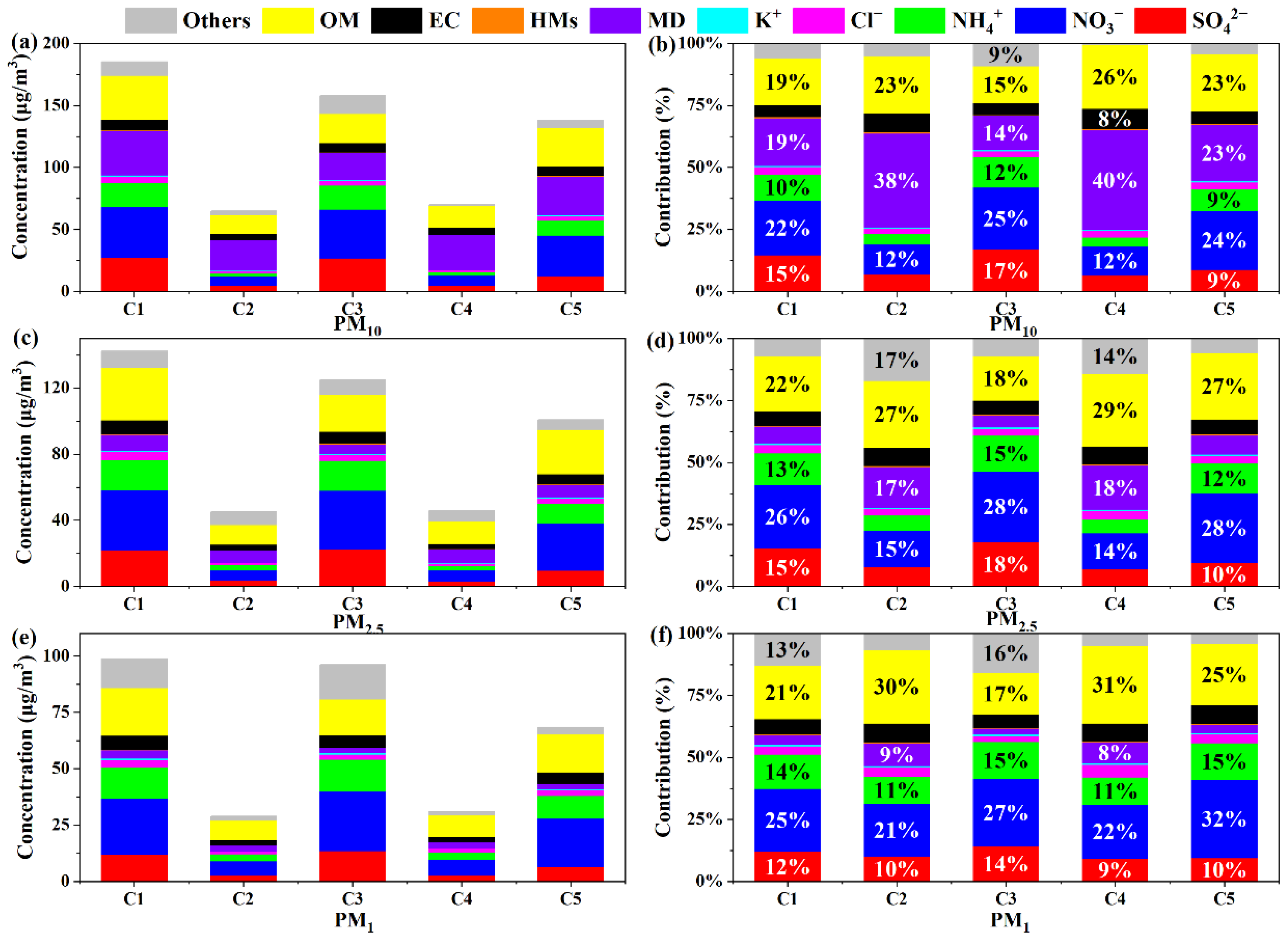
3.3. PM Source Appointment

The US EPA 5.0 model was used to apportion the contribution sources of airborne particles based on the dataset of 82 effective samples from 21 December 2019 to 17 January 2020. Because the source profiles of PM₁₀, PM_2.5 and PM₁ were quite similar [32,37,63,64,65], the PM data from different size particulates (PM₁₀, PM_2.5 and PM₁) were combined and imputed into PMF in this study as was the case in other previous studies [38,63,64,65]. The contribution of apportioned sources calculated by evaluating the annual average concentrations are presented in Figure 6. The source apportionment results of PM are shown in Figure S3 in the Supplementary Materials. The apportioned sources and their contributions are summarized as follows:

Factor 1 represents traffic sources with high loadings of OC, EC, and the heavy metals of Zn, Cu, Mn, and Pb (Figure S3) [66]. The annual average concentration of traffic sources contributed to 23.0–24.4% of the PM mass. In addition, secondary aerosols can be transformed by the precursors SO₂, NO_X, VOCs and NH₃, and motor vehicle exhaust was one of the most important NO_X and VOCs emission sources in urban areas [67,68,69]. Consequently, the contribution of this factor to PM would be much higher when considering the secondary transformation of gaseous precursors. Factor 2 and Factor 6 explained 2.4%, 0.7%, 0.8% and 3.6%, 3.2%, 1.9% of the total variance of PM₁₀, PM_2.5, and PM₁, respectively. The characteristics of these factors included high loadings of typical elements which were associated with industrial sources, including Co, Ni, Cr, and Cd. Xinxiang is known as the capital of the battery industry and produces various types of batteries including nickel–cadmium batteries, Ternary lithium batteries, lithium iron phosphate batteries, and lead batteries [51]. Cement production, and a non-ferrous smelter were also located around observation site. Consequently, pollutants emissions for industrial processes slightly increased the PM concentration.

Factor 3 was identified as combustion sources, which mainly included coal combustion and biomass burning. Coal combustion was characterized by a high content of chloride, OC, and EC [18,70]. Biomass burning contained a significant amount of K⁺, which was generally considered as a good tracer of biomasses [71]. Combustion source were found to have a significantly lower contribution to the PM₁₀ (12.8%) in Xinxiang than those in smaller particles (22.7% for PM_2.5 and 25.4% for PM₁), demonstrating that much smaller sized airborne particles were emissions from combustion processes. The findings were in accordance with the results reported in previous studies [32,37].

The fourth factor was identified as dust featured with abundant concentrations of Ca²⁺, Mg²⁺, Al, Fe, Mn, and Ti. The elements of Fe and Mn were partly derived from soil dust released by urban subways and ground vehicles as proposed in previous studies [72,73]. The chemical species Mg²⁺, Ca²⁺ can be regarded as good tracers of construction dust, soil dust and road dust according to previous studies [8]. Therefore, this source was apportioned as dust, which included soil dust, construction dust and transportation dust. The average contribution of dust to PM₁₀ (19.1%) was higher than that in PM_2.5 (3.9%) and PM₁ (2.2%). These results demonstrated that fugitive dust was more likely to be enriched in course particles, which is consistent with the above discussion.

The fifth factor was associated with secondary aerosols because of the high loadings of nitrate, sulfate, and ammonium as only minor OC mass (Figure S3), which can be classified as a secondary inorganic aerosol (SNA) source [74,75]. The secondary aerosol (SA) was identified as the dominant source of multi-size particles, and their contributions to PM mass ranged from 37.8% to 46.7% (Figure 6). Similar to the variation characteristics in combustion sources, a higher concentration was found in terms of smaller-size particles, which is consistent with many studies conducted previously in North China [32,37].

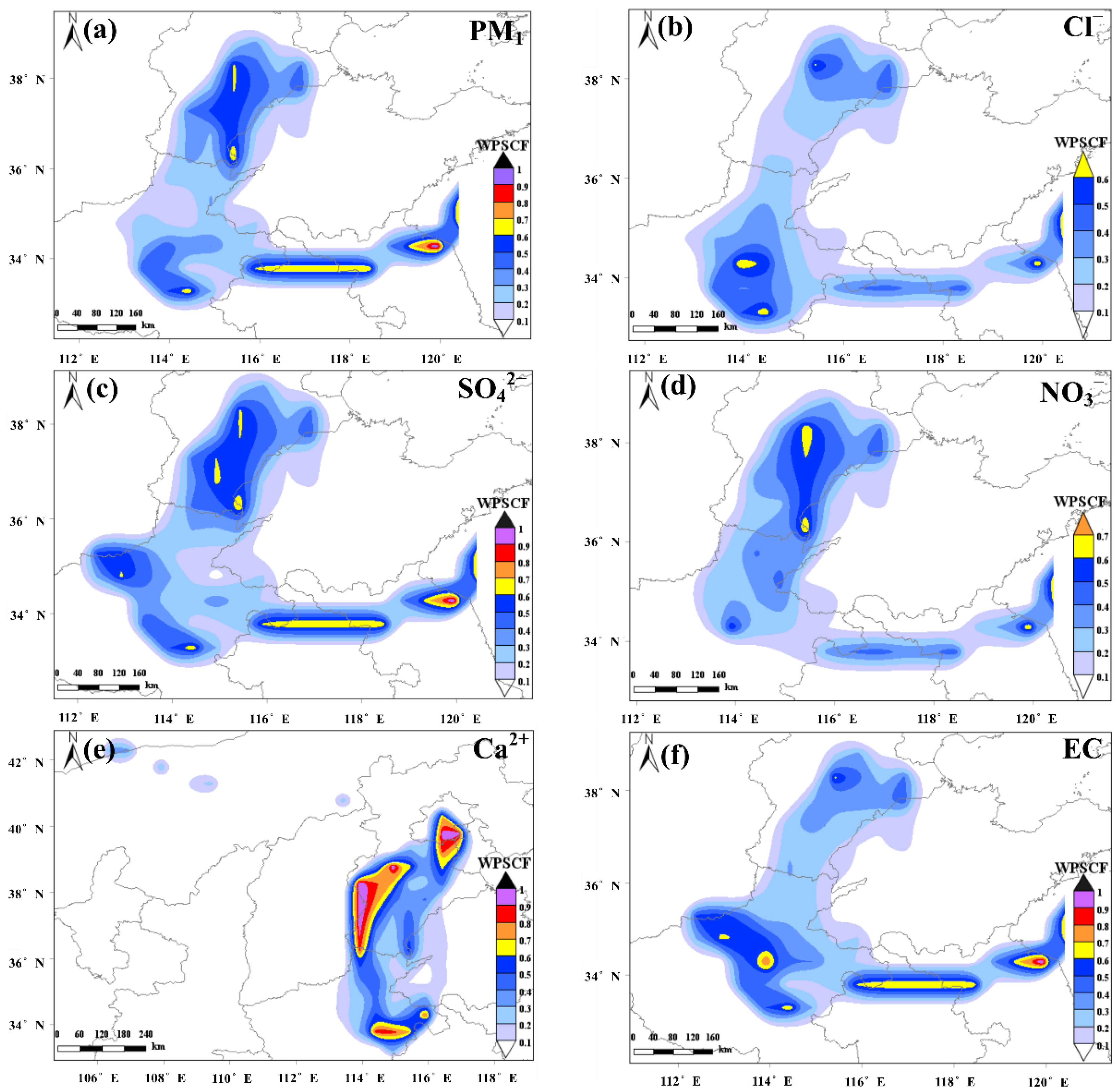
3.4. Geographical Origins of PM

The 48 h air mass backward trajectories analysis from Xinxiang during the whole observation period is shown in Figure 7. Five clusters were found in this study named C1, C2, C3, C4, and C5, which accounted for 44.49%, 9.38%, 36.46%, 4.17%, and 5.51% of the overall trajectories, respectively. Cluster 1 (blue line) primarily originated from the west of Shandong province, travelling over some heavily polluted cities in the east of Henan province [5,76]. The cluster C2 (green line) mainly derived from Mongolia and moved at relatively great speeds and height, while cluster C3 (claybank line) originated from the north, began in Hebei province and crossed over several heavy polluted cities covering Handan, Xingtai, Anyang, which are typical heavily polluted areas [3,13,32]. The cluster C4 (Blank line) moved at the fastest wind speeds and highest height, and was mainly derived from Xinjiang, Gansu, and Inner Mongolia and passed over the Shaanxi and Shanxi provinces before arriving at the research area. The cluster C5 (red line) came from the south and crossed over Hubei province and several cities in the South and Central Henan province.

As shown in Figure 7 and Figure 8, the pollutant concentrations in cluster C1 were higher than the other clusters, and the average mass concentrations of PM₁₀, PM_2.5, and PM₁ were 183.59, 141.89, and 97.93 μg m⁻³, respectively. The chemical compositions in multi-size particles exhibited varying trajectory-dependence characteristics. Cluster C1 featured a high concentration and proportion of sulfate, nitration, and ammonium. Similar chemical species variation patterns were also found in high concentration air masses associated with cluster C3 (95.52–157.73 μg m⁻³) and C5 (67.03–138.33 μg m⁻³) (Figure 7 and Figure 8). The entrained particulate matter of cluster 1, cluster 3, and cluster 5, with eastern, northern and southern sources combined with the secondary formation by gaseous precursors elevated the PM concentration at the sampling cities [2,8]. Compared with cluster C1 and C5, the concentrations and proportion of sulfate in cluster C3 were significantly higher (Figure 8). In comparison, the lowest concentrations of PM₁₀ (63.45 μg m⁻³), PM_2.5 (44.96 μg m⁻³), and PM₁ (28.81 μg m⁻³) were found in trajectories associated with cluster C2. PM associated with cluster C1 was characterized by a high concentration and proportion of MD (Figure 8), demonstrating that dust and sand from Inner Mongolia elevated the PM concentration in Xinxiang [2]. Similar variation patterns of species were also observed in PM with C4. Among the five clusters, the common features of species were that MD was mainly enriched in PM₁₀, and OC and SNA were mainly distributed in small–size particles. These results were consistent with previous studies [24,27,32,37].

The WPSCF analysis model is often used to identify the influence of regional transport and explore the potential source region [2]. Some studies evaluated the contribution of PM_2.5 in North China, and the conclusions exhibited obvious regional transport contributions to PM_2.5 [77,78]. Though PM₁ has been confirmed as more susceptible to regional transport, the related studies in Xinxiang are scarce. Therefore, a WPSCF analysis of PM₁ and its primary compositions was conducted and the results are shown in Figure 9. The WPSCF results showed that PM₁ and its chemical species (except Ca²⁺) had similar spatial potential contribution areas. The patterns of regional transport of all species were found at the observed site, which coincided with previous studies [2,32,77]. The air masses from the east, northeast and southeast of the observed site had a major influence on the research region and the potential contribution areas included Jiangsu, Anhui, and Hebei province. The air masses from these regions entrained with a high concentration of PM and gaseous precursor can induce the persistent accumulation of PM₁ and generate regional pollution episodes. For Ca²⁺, the relatively high WPSCF value was observed in the north and southeast of Xinxiang, covering the Hebei and Henan province. Overall, the results discussed above illustrated that PM₁ was more strongly influenced by regional transport due to its finer aerodynamic diameter [37].

4. Conclusions

Xinxiang has experienced heavy particulate matter pollution during recent years. In this study, PM₁₀, PM_2.5, and PM₁ samples were synchronously collected from 21 December 2019 to 17 January 2020 in Xinxiang. The average mass concentration of PM₁₀, PM_2.5, and PM₁ were as high as 155.53 ± 66.22 μg m⁻³, 120.07 ± 52.86 μg m⁻³, and 85.64 ± 41.49 μg m⁻³ during the observation period, respectively. The observational average concentration of PM_2.5 was about 1.6 times the National Ambient Air Standard (NAAQS) (GB3095—2012) daily average limit (75 μg m⁻³), demonstrating the seriousness of airborne particles pollution in winter in Xinxiang. The average PM₁/PM_2.5 ratio and PM_2.5/PM₁₀ were about 71.3% and 77.2%, respectively, and the ratios all correlated with RH and negatively correlated with WS to a certain extent.

Nearly all of the chemical compositions in PM₁₀, PM_2.5 and PM₁ increased continuously and obviously with the aggravation of PM pollution. From the clean period to the slightly polluted period, the contribution of SNA increased by 16–48%; therein, the enhancement of nitrate was significantly larger than sulfate. However, the increase in nitrate was lower than sulfate from moderate pollution to heavy pollution.

Three pollution periods were found during the entire observation period. During pollution episode 1, the rapid transformation of sulfate dominated the formation of this haze pollution. High concentrations of PM in pollution period 2 could be caused by the dust and combustion sources. Pollution episode 3 was characterized by the common formation of sulfate and nitrate.

The results apportioned from the PMF model showed that the major PM sources were as follows: traffic source, combustion source, secondary aerosols, industrial source, and fugitive dust in Xinxiang. The contributions of combustion source and secondary aerosols were found to be higher in smaller particles (PM_2.5 and PM₁), while the contribution of fugitive dust was higher in PM₁₀. The potential source regions were mainly distributed in Hebei, Jiangsu, Anhui and Hebei. This work offered first-hand details on PM₁₀, PM_2.5 and PM₁ in a heavily polluted city in China, which can be helpful in elucidating components and sources of different size particles and assist in the alleviation of PM pollution in polluted areas around world. In future studies, high-temporal resolution (such as 1hour or several minutes), a long time scale and multi-size PM online observations can provided more information on the secondary formation mechanism, haze evolution, and size distribution characteristics.

References

1. Hong, Y.; Cao, F.; Fan, M.-Y.; Lin, Y.-C.; Gul, C.; Yu, M.; Wu, X.; Zhai, X.; Zhang, Y.-L. Impacts of chemical degradation of levoglucosan on quantifying biomass burning contribution to carbonaceous aerosols: A case study in Northeast China. Sci. Total Environ. 2022, 819, 152007. [Google Scholar] [CrossRef] [PubMed]
2. Liu, H.; Tian, H.; Zhang, K.; Liu, S.; Cheng, K.; Yin, S.; Liu, Y.; Liu, X.; Wu, Y.; Liu, W.; et al. Seasonal variation, formation mechanisms and potential sources of PM2.5 in two typical cities in the Central Plains Urban Agglomeration, China. Sci. Total Environ. 2018, 657, 657–670. [Google Scholar] [CrossRef]
3. Zhang, J.; Yuan, Q.; Liu, L.; Wang, Y.; Zhang, Y.; Xu, L.; Pang, Y.; Zhu, Y.; Niu, H.; Shao, L.; et al. Trans-Regional Transport of Haze Particles from the North China Plain to Yangtze River Delta during Winter. J. Geophys. Res. Atmos. 2021, 126, e2020JD033778. [Google Scholar] [CrossRef]
4. Zhao, B.; Zhao, J.; Zha, H.; Hu, R.; Liu, Y.; Liang, C.; Shi, H.; Chen, S.; Guo, Y.; Zhang, D.; et al. Health Benefits and Costs of Clean Heating Renovation: An Integrated Assessment in a Major Chinese City. Environ. Sci. Technol. 2021, 55, 10046–10055. [Google Scholar] [CrossRef]
5. Wang, Y.; Li, W.; Gao, W.; Liu, Z.; Tian, S.; Shen, R.; Ji, D.; Wang, S.; Wang, L.; Tang, G.; et al. Trends in particulate matter and its chemical compositions in China from 2013–2017. Sci. China Earth Sci. 2019, 62, 1857–1871. [Google Scholar] [CrossRef]
6. Liu, J.; Chen, Y.; Cao, H.; Zhang, A. Burden of typical diseases attributed to the sources of PM2.5-bound toxic metals in Beijing: An integrated approach to source apportionment and QALYs. Environ. Int. 2019, 131, 105041. [Google Scholar] [CrossRef] [PubMed]
7. Zhao, B.; Zheng, H.; Wang, S.; Smith, K.R.; Lu, X.; Aunan, K.; Gu, Y.; Wang, Y.; Ding, D.; Xing, J.; et al. Change in household fuels dominates the decrease in PM2.5 exposure and premature mortality in China in 2005–2015. Proc. Natl. Acad. Sci. USA 2018, 115, 12401–12406. [Google Scholar] [CrossRef] [PubMed]
8. Huang, X.; Liu, Z.; Liu, J.; Hu, B.; Wen, T.; Tang, G.; Zhang, J.; Wu, F.; Ji, D.; Wang, L.; et al. Chemical characterization and source identification of PM2.5 at multiple sites in the Beijing–Tianjin–Hebei region, China. Atmos. Chem. Phys. 2017, 17, 12941–12962. [Google Scholar] [CrossRef]
9. Jiang, H.; Liao, H.; Pye, H.O.T.; Wu, S.; Mickley, L.J.; Seinfeld, J.H.; Zhang, X.Y. Projected effect of 2000–2050 changes in climate and emissions on aerosol levels in China and associated transboundary transport. Atmos. Chem. Phys. 2013, 13, 7937–7960. [Google Scholar] [CrossRef]
10. Li, Y.; Huang, H.X.; Griffith, S.M.; Wu, C.; Lau, A.K.; Yu, J.Z. Quantifying the relationship between visibility degradation and PM2.5 constituents at a suburban site in Hong Kong: Differentiating contributions from hydrophilic and hydrophobic organic compounds. Sci. Total Environ. 2017, 575, 1571–1581. [Google Scholar] [CrossRef]
11. Geng, G.; Zheng, Y.; Zhang, Q.; Xue, T.; Zhao, H.; Tong, D.; Zheng, B.; Li, M.; Liu, F.; Hong, C.; et al. Drivers of PM2.5 air pollution deaths in China 2002–2017. Nat. Geosci. 2021, 14, 645–650. [Google Scholar] [CrossRef]
12. Li, J.; Zhang, Y.-L.; Cao, F.; Zhang, W.; Fan, M.; Lee, X.; Michalski, G. Stable Sulfur Isotopes Revealed a Major Role of Transition-Metal Ion-Catalyzed SO2 Oxidation in Haze Episodes. Environ. Sci. Technol. 2020, 54, 2626–2634. [Google Scholar] [CrossRef] [PubMed]
13. Li, M.; Wang, L.; Liu, J.; Gao, W.; Song, T.; Sun, Y.; Li, L.; Li, X.; Wang, Y.; Liu, L.; et al. Exploring the regional pollution characteristics and meteorological formation mechanism of PM2.5 in North China during 2013–2017. Environ. Int. 2019, 134, 105283. [Google Scholar] [CrossRef]
14. Liu, T.; Clegg, S.L.; Abbatt, J.P.D. Fast oxidation of sulfur dioxide by hydrogen peroxide in deliquesced aerosol particles. Proc. Natl. Acad. Sci. USA 2020, 117, 1354–1359. [Google Scholar] [CrossRef]
15. Zhang, F.; Wang, Y.; Peng, J.; Chen, L.; Sun, Y.; Duan, L.; Ge, X.; Li, Y.; Zhao, J.; Liu, C.; et al. An unexpected catalyst dominates formation and radiative forcing of regional haze. Proc. Natl. Acad. Sci. USA 2020, 117, 3960–3966. [Google Scholar] [CrossRef] [PubMed]
16. Wang, J.; Ye, J.; Zhang, Q.; Zhao, J.; Wu, Y.; Li, J.; Liu, D.; Li, W.; Zhang, Y.; Wu, C.; et al. Aqueous production of secondary organic aerosol from fossil-fuel emissions in winter Beijing haze. Proc. Natl. Acad. Sci. USA 2021, 118, e2022179118. [Google Scholar] [CrossRef]
17. Zhang, Y.; Ren, H.; Sun, Y.; Cao, F.; Chang, Y.; Liu, S.; Lee, X.; Agrios, K.; Kawamura, K.; Liu, D.; et al. High Contribution of Nonfossil Sources to Submicrometer Organic Aerosols in Beijing, China. Environ. Sci. Technol. 2017, 51, 7842–7852. [Google Scholar] [CrossRef]
18. Zhou, W.; Wang, Q.; Zhao, X.; Xu, W.; Chen, C.; Du, W.; Zhao, J.; Canonaco, F.; Prévôt, A.S.H.; Fu, P.; et al. Characterization and source apportionment of organic aerosol at 260 m on a meteorological tower in Beijing, China. Atmos. Chem. Phys. 2018, 18, 3951–3968. [Google Scholar] [CrossRef]
19. Rattanavaraha, W.; Canagaratna, M.R.; Budisulistiorini, S.H.; Croteau, P.L.; Baumann, K.; Canonaco, F.; Prevot, A.S.; Edgerton, E.S.; Zhang, Z.; Jayne, J.T.; et al. Source apportionment of submicron organic aerosol collected from Atlanta, Georgia, during 2014–2015 using the aerosol chemical speciation monitor (ACSM). Atmos. Environ. 2017, 167, 389–402. [Google Scholar] [CrossRef]
20. Du, A.; Li, Y.; Sun, J.; Zhang, Z.; You, B.; Li, Z.; Chen, C.; Li, J.; Qiu, Y.; Liu, X.; et al. Rapid transition of aerosol optical properties and water-soluble organic aerosols in cold season in Fenwei Plain. Sci. Total Environ. 2022, 829, 154661. [Google Scholar] [CrossRef]
21. Sun, Y.; Lei, L.; Zhou, W.; Chen, C.; He, Y.; Sun, J.; Li, Z.; Xu, W.; Wang, Q.; Ji, D.; et al. A chemical cocktail during the COVID-19 outbreak in Beijing, China: Insights from six-year aerosol particle composition measurements during the Chinese New Year holiday. Sci. Total Environ. 2020, 742, 140739. [Google Scholar] [CrossRef]
22. Yan, G.; Zhang, J.; Zhang, P.; Cao, Z.; Zhu, G.; Liu, Z.; Wang, Y. Episode-Based Analysis of Size-Resolved Carbonaceous Aerosol Compositions in Wintertime of Xinxiang: Implication for the Haze Formation Processes in Central China. Appl. Sci. 2020, 10, 3498. [Google Scholar] [CrossRef]
23. Feng, J.; Yu, H.; Su, X.; Liu, S.; Li, Y.; Pan, Y.; Sun, J.-H. Chemical composition and source apportionment of PM2.5 during Chinese Spring Festival at Xinxiang, a heavily polluted city in North China: Fireworks and health risks. Atmos. Res. 2016, 182, 176–188. [Google Scholar] [CrossRef]
24. Shao, P.; Tian, H.; Sun, Y.; Liu, H.; Wu, B.; Liu, S.; Liu, X.; Wu, Y.; Liang, W.; Wang, Y.; et al. Characterizing remarkable changes of severe haze events and chemical compositions in multi-size airborne particles (PM1, PM2.5 and PM10) from January 2013 to 2016–2017 winter in Beijing, China. Atmos. Environ. 2018, 189, 133–144. [Google Scholar] [CrossRef]
25. Gao, J.; Wang, K.; Wang, Y.; Liu, S.; Zhu, C.; Hao, J.; Liu, H.; Hua, S.; Tian, H. Temporal-spatial characteristics and source apportionment of PM2.5 as well as its associated chemical species in the Beijing-Tianjin-Hebei region of China. Environ. Pollut. 2017, 233, 714–724. [Google Scholar] [CrossRef]
26. Aiken, A.C.; DeCarlo, P.F.; Kroll, J.H.; Worsnop, D.R.; Huffman, J.A.; Docherty, K.S.; Ulbrich, I.M.; Mohr, C.; Kimmel, J.R.; Sueper, D.; et al. O/C and OM/OC Ratios of Primary, Secondary, and Ambient Organic Aerosols with High-Resolution Time-of-Flight Aerosol Mass Spectrometry. Environ. Sci. Technol. 2008, 42, 4478–4485. [Google Scholar] [CrossRef]
27. Dai, Q.; Bi, X.; Liu, B.; Li, L.; Ding, J.; Song, W.; Bi, S.; Schulze, B.C.; Song, C.; Wu, J.; et al. Chemical nature of PM2.5 and PM10 in Xi’an, China: Insights into primary emissions and secondary particle formation. Environ. Pollut. 2018, 240, 155–166. [Google Scholar] [CrossRef]
28. Sun, Y.; Du, W.; Fu, P.; Wang, Q.; Li, J.; Ge, X.; Zhang, Q.; Zhu, C.; Ren, L.; Xu, W.; et al. Primary and secondary aerosols in Beijing in winter: Sources, variations and processes. Atmos. Chem. Phys. 2016, 16, 8309–8329. [Google Scholar] [CrossRef]
29. Bressi, M.; Sciare, J.; Ghersi, V.; Bonnaire, N.; Nicolas, J.B.; Petit, J.-E.; Moukhtar, S.; Rosso, A.; Mihalopoulos, N.; Féron, A. A one-year comprehensive chemical characterisation of fine aerosol (PM2.5) at urban, suburban and rural background sites in the region of Paris (France). Atmos. Chem. Phys. 2013, 13, 7825–7844. [Google Scholar] [CrossRef]
30. Tan, T.; Hu, M.; Li, M.; Guo, Q.; Wu, Y.; Fang, X.; Gu, F.; Wang, Y.; Wu, Z. New insight into PM2.5 pollution patterns in Beijing based on one-year measurement of chemical compositions. Sci. Total Environ. 2018, 621, 734–743. [Google Scholar] [CrossRef]
31. Taylor, S.R.; McLennan, S.M. The continental crust: Its composition and evolution. J. Jeol. 1985, 94, 57–72. [Google Scholar]
32. Chen, C.; Zhang, H.; Li, H.; Wu, N.; Zhang, Q. Chemical characteristics and source apportionment of ambient PM1.0 and PM2.5 in a polluted city in North China plain. Atmos. Environ. 2020, 242, 117867. [Google Scholar] [CrossRef]
33. Gu, Y.; Liu, B.; Dai, Q.; Zhang, Y.; Zhou, M.; Feng, Y.; Hopke, P.K. Multiply improved positive matrix factorization for source apportionment of volatile organic compounds during the COVID-19 shutdown in Tianjin, China. Environ. Int. 2021, 158, 106979. [Google Scholar] [CrossRef] [PubMed]
34. United States Environmental Protection Agency (USEPA). Positive Matrix Factorization (PMF) 5.0 Fundamentals and User Guide; US Environmental Protection Agency: Washington, DC, USA, 2014.
35. Polissar, A.V.; Hopke, P.K.; Paatero, P.; Malm, W.C.; Sisler, J.F. Atmospheric aerosol over Alaska: 2. Elemental composition and sources. J. Geophys. Res. Earth Surf. 1998, 103, 19045–19057. [Google Scholar] [CrossRef]
36. Liu, J.W.; Chen, Y.J.; Chao, S.H.; Chao, H.B.; Zhang, A.C.; Yang, Y. Emission control priority of PM2.5-bound heavy metals in different seasons: A comprehensive analysis from health risk perspective. Sci. Total Environ. 2018, 644, 20–30. [Google Scholar] [CrossRef]
37. Zhang, Y.; Lang, J.; Cheng, S.; Li, S.; Zhou, Y.; Chen, D.; Zhang, H.; Wang, H. Chemical composition and sources of PM1 and PM2.5 in Beijing in autumn. Sci. Total Environ. 2018, 630, 72–82. [Google Scholar] [CrossRef] [PubMed]
38. Lang, J.; Li, S.; Cheng, S.; Zhou, Y.; Chen, D.; Zhang, Y.; Zhang, H.; Wang, H. Chemical Characteristics and Sources of Submicron Particles in a City with Heavy Pollution in China. Atmosphere 2018, 9, 388. [Google Scholar] [CrossRef]
39. Ji, D.; Gao, W.; Maenhaut, W.; He, J.; Wang, Z.; Li, J.; Du, W.; Wang, L.; Sun, Y.; Xin, J.; et al. Impact of air pollution control measures and regional transport on carbonaceous aerosols in fine particulate matter in urban Beijing, China: Insights gained from long-term measurement. Atmos. Chem. Phys. 2019, 19, 8569–8590. [Google Scholar] [CrossRef]
40. Zhang, Y.; Chen, J.; Yang, H.; Li, R.; Yu, Q. Seasonal variation and potential source regions of PM2.5-bound PAHs in the megacity Beijing, China: Impact of regional transport. Environ. Pollut. 2017, 231, 329–338. [Google Scholar] [CrossRef]
41. Wang, Y.Q.; Zhang, X.Y.; Draxler, R.R. TrajStat: GIS-based software that uses various trajectory statistical analysis methods to identify potential sources from long-term air pollution measurement data. Environ. Model. Softw. 2009, 24, 938–939. [Google Scholar] [CrossRef]
42. Du, T.; Wang, M.; Guan, X.; Zhang, M.; Zeng, H.; Chang, Y.; Zhang, L.; Tian, P.; Shi, J.; Tang, C. Characteristics and Formation Mechanisms of Winter Particulate Pollution in Lanzhou, Northwest China. J. Geophys. Res. Atmos. 2020, 125, e2020JD033369. [Google Scholar] [CrossRef]
43. Li, Y.; Du, A.; Li, Z.; Li, J.; Chen, C.; Sun, J.; Qiu, Y.; Zhang, Z.; Wang, Q.; Xu, W.; et al. Investigation of sources and formation mechanisms of fine particles and organic aerosols in cold season in Fenhe Plain, China. Atmos. Res. 2022, 268, 106018. [Google Scholar] [CrossRef]
44. Guo, S.; Hu, M.; Wang, Z.B.; Slanina, J.; Zhao, Y.L. Size-resolved aerosol water-soluble ionic compositions in the summer of Beijing: Implication of regional secondary formation. Atmos. Chem. Phys. 2010, 10, 947–959. [Google Scholar] [CrossRef]
45. Cheng, Y.; Zheng, G.; Wei, C.; Mu, Q.; Zheng, B.; Wang, Z.; Gao, M.; Zhang, Q.; He, K.; Carmichael, G.; et al. Reactive nitrogen chemistry in aerosol water as a source of sulfate during haze events in China. Sci. Adv. 2016, 2, e1601530. [Google Scholar] [CrossRef] [PubMed]
46. Wang, G.; Zhang, R.; Gomez, M.E.; Yang, L.; Zamora, M.L.; Hu, M.; Lin, Y.; Peng, J.; Guo, S.; Meng, J.; et al. Persistent sulfate formation from London Fog to Chinese haze. Proc. Natl. Acad. Sci. USA 2016, 113, 13630–13635. [Google Scholar] [CrossRef] [PubMed]
47. Gao, J.; Tian, H.; Cheng, K.; Lu, L.; Wang, Y.; Wu, Y.; Zhu, C.; Liu, K.; Zhou, J.; Liu, X.; et al. Seasonal and spatial variation of trace elements in multi-size airborne particulate matters of Beijing, China: Mass concentration, enrichment characteristics, source apportionment, chemical speciation and bioavailability. Atmos. Environ. 2014, 99, 257–265. [Google Scholar] [CrossRef]
48. Tian, H.Z.; Zhu, C.Y.; Gao, J.J.; Cheng, K.; Hao, J.M.; Wang, K.; Hua, S.B.; Wang, Y.; Zhou, J.R. Quantitative assessment of atmospheric emissions of toxic heavy metals from anthropogenic sources in China: Historical trend, spatial distribution, uncertainties, and control policies. Atmos. Chem. Phys. 2015, 15, 10127–10147. [Google Scholar] [CrossRef]
49. Zhu, C.; Tian, H.; Hao, J. Global anthropogenic atmospheric emission inventory of twelve typical hazardous trace elements, 1995–2012. Atmos. Environ. 2020, 220, 117061. [Google Scholar] [CrossRef]
50. Zhu, C.; Tian, H.; Hao, Y.; Gao, J.; Hao, J.; Wang, Y.; Hua, S.; Wang, K.; Liu, H. A high-resolution emission inventory of anthropogenic trace elements in Beijing-Tianjin-Hebei (BTH) region of China. Atmos. Environ. 2018, 191, 452–462. [Google Scholar] [CrossRef]
51. Liu, H.J.; Jia, M.K.; Liu, Y.L.; Zhao, Y.J.; Zheng, A.H.; Liu, H.Z.; Xu, S.Y.; Xiao, Q.Q.; Su, X.Y.; Ren, Y. Seasonal variation, source identification, and health risk of PM2.5–bound metals in Xinxiang. Environ. Sci. 2021, 42, 4140–4150. (In Chinese) [Google Scholar] [CrossRef]
52. Cui, Y.; Ji, D.; Maenhaut, W.; Gao, W.; Zhang, R.; Wang, Y. Levels and sources of hourly PM2.5-related elements during the control period of the COVID-19 pandemic at a rural site between Beijing and Tianjin. Sci. Total Environ. 2020, 744, 140840. [Google Scholar] [CrossRef]
53. Kong, L.; Feng, M.; Liu, Y.; Zhang, Y.; Zhang, C.; Li, C.; Qu, Y.; An, J.; Liu, X.; Tan, Q.; et al. Elucidating the pollution characteristics of nitrate, sulfate and ammonium in PM2.5 in Chengdu, southwest China, based on 3-year measurements. Atmos. Chem. Phys. 2020, 20, 11181–11199. [Google Scholar] [CrossRef]
54. Zhang, X.; Li, Z.; Wang, F.; Song, M.; Zhou, X.; Ming, J. Carbonaceous Aerosols in PM1, PM2.5, and PM10 Size Fractions over the Lanzhou City, Northwest China. Atmosphere 2020, 11, 1368. [Google Scholar] [CrossRef]
55. Vu, T.V.; Shi, Z.; Cheng, J.; Zhang, Q.; He, K.; Wang, S.; Harrison, R.M. Assessing the impact of clean air action on air quality trends in Beijing using a machine learning technique. Atmos. Chem. Phys. 2019, 19, 11303–11314. [Google Scholar] [CrossRef]
56. Sun, Y.; Chen, C.; Zhang, Y.; Xu, W.; Zhou, L.; Cheng, X.; Zheng, H.; Ji, D.; Li, J.; Tang, X.; et al. Rapid formation and evolution of an extreme haze episode in Northern China during winter 2015. Sci. Rep. 2016, 6, 27151. [Google Scholar] [CrossRef] [PubMed]
57. Fu, X.; Wang, T.; Gao, J.; Wang, P.; Liu, Y.; Wang, S.; Zhao, B.; Xue, L. Persistent Heavy Winter Nitrate Pollution Driven by Increased Photochemical Oxidants in Northern China. Environ. Sci. Technol. 2020, 54, 3881–3889. [Google Scholar] [CrossRef]
58. Sun, Y.; Zhuang, G.; Tang, A.; Wang, Y.; An, Z. Chemical Characteristics of PM2.5 and PM10 in Haze−Fog Episodes in Beijing. Environ. Sci. Technol. 2006, 40, 3148–3155. [Google Scholar] [CrossRef]
59. Duan, J.; Tan, J. Atmospheric heavy metals and Arsenic in China: Situation, sources and control policies. Atmos. Environ. 2013, 74, 93–101. [Google Scholar] [CrossRef]
60. Blitz, M.A.; Hughes, K.J.; Pilling, M.J. Determination of the High-Pressure Limiting Rate Coefficient and the Enthalpy of Reaction for OH + SO2. J. Phys. Chem. A 2003, 107, 1971–1978. [Google Scholar] [CrossRef]
61. Calvert, J.G.; Stockwell, W.R. Acid generation in the troposphere by gas-phase chemistry. Environ. Sci. Technol. 1983, 17, 428A–443A. [Google Scholar] [CrossRef]
62. Ianniello, A.; Spataro, F.; Esposito, G.; Allegrini, I.; Hu, M.; Zhu, T. Chemical characteristics of inorganic ammonium salts in PM2.5 in the atmosphere of Beijing (China). Atmos. Chem. Phys. 2011, 11, 10803–10822. [Google Scholar] [CrossRef] [Green Version]
63. Tian, Y.Z.; Wang, J.; Peng, X.; Shi, G.L.; Feng, Y.C. Estimation of the direct and indirect impacts of fireworks on the physicochemical characteristics of atmospheric PM10 and PM2.5. Atmos. Chem. Phys. 2014, 14, 9469–9479. [Google Scholar] [CrossRef]
64. Pérez, N.; Pey, J.; Reche, C.; Cortés, J.; Alastuey, A.; Querol, X. Impact of harbour emissions on ambient PM10 and PM2.5 in Barcelona (Spain): Evidences of secondary aerosol formation within the urban area. Sci. Total Environ. 2016, 571, 237–250. [Google Scholar] [CrossRef] [PubMed]
65. Pandolfi, M.; Castanedo, Y.G.; Alastuey, A.; de la Rosa, J.D.; Mantilla, E.; de la Campa, A.M.S.; Querol, X.; Pey, J.; Amato, F.; Moreno, T. Source apportionment of PM10 and PM2.5 at multiple sites in the strait of Gibraltar by PMF: Impact of shipping emissions. Environ. Sci. Pollut. Res. 2010, 18, 260–269. [Google Scholar] [CrossRef]
66. Chang, Y.; Huang, K.; Xie, M.; Deng, C.; Zou, Z.; Liu, S.; Zhang, Y. First long-term and near real-time measurement of trace elements in China’s urban atmosphere: Temporal variability, source apportionment and precipitation effect. Atmos. Chem. Phys. 2018, 18, 11793–11812. [Google Scholar] [CrossRef]
67. Gu, X.; Yin, S.; Lu, X.; Zhang, H.; Wang, L.; Bai, L.; Wang, C.; Zhang, R.; Yuan, M. Recent development of a refined multiple air pollutant emission inventory of vehicles in the Central Plains of China. J. Environ. Sci. 2019, 84, 80–96. [Google Scholar] [CrossRef]
68. Jiang, P.; Zhong, X.; Li, L. On-road vehicle emission inventory and its spatio-temporal variations in North China Plain. Environ. Pollut. 2020, 267, 115639. [Google Scholar] [CrossRef] [PubMed]
69. Liao, K.; Chen, Q.; Liu, Y.; Li, Y.J.; Lambe, A.T.; Zhu, T.; Huang, R.-J.; Zheng, Y.; Cheng, X.; Miao, R.; et al. Secondary Organic Aerosol Formation of Fleet Vehicle Emissions in China: Potential Seasonality of Spatial Distributions. Environ. Sci. Technol. 2021, 55, 7276–7286. [Google Scholar] [CrossRef]
70. Theodosi, C.; Tsagkaraki, M.; Zarmpas, P.; Grivas, G.; Liakakou, E.; Paraskevopoulou, D.; Lianou, M.; Gerasopoulos, E.; Mihalopoulos, N. Multi-year chemical composition of the fine-aerosol fraction in Athens, Greece, with emphasis on the contribution of residential heating in wintertime. Atmos. Chem. Phys. 2018, 18, 14371–14391. [Google Scholar] [CrossRef]
71. Huang, S.; Wu, Z.; Poulain, L.; van Pinxteren, M.; Merkel, M.; Assmann, D.; Herrmann, H.; Wiedensohler, A. Source apportionment of the organic aerosol over the Atlantic Ocean from 53° N to 53° S: Significant contributions from marine emissions and long-range transport. Atmos. Chem. Phys. 2018, 18, 18043–18062. [Google Scholar] [CrossRef]
72. Mugica-Álvarez, V.; Figueroa-Lara, J.; Romero-Romo, M.; Sepúlveda-Sánchez, J.; López-Moreno, T. Concentrations and properties of airborne particles in the Mexico City subway system. Atmos. Environ. 2012, 49, 284–293. [Google Scholar] [CrossRef]
73. Taghvaee, S.; Sowlat, M.H.; Mousavi, A.; Hassanvand, M.S.; Yunesian, M.; Naddafi, K.; Sioutas, C. Source apportionment of ambient PM2.5 in two locations in central Tehran using the Positive Matrix Factorization (PMF) model. Sci. Total Environ. 2018, 628–629, 672–686. [Google Scholar] [CrossRef] [PubMed]
74. Huang, X.-F.; Zou, B.-B.; He, L.-Y.; Hu, M.; Prévôt, A.S.H.; Zhang, Y.-H. Exploration of PM2.5 sources on the regional scale in the Pearl River Delta based on ME-2 modeling. Atmos. Chem. Phys. 2018, 18, 11563–11580. [Google Scholar] [CrossRef]
75. Zhou, S.; Davy, P.K.; Huang, M.; Duan, J.; Wang, X.; Fan, Q.; Chang, M.; Liu, Y.; Chen, W.; Xie, S.; et al. High-resolution sampling and analysis of ambient particulate matter in the Pearl River Delta region of southern China: Source apportionment and health risk implications. Atmos. Chem. Phys. 2018, 18, 2049–2064. [Google Scholar] [CrossRef]
76. Dao, X.; Ji, D.; Zhang, X.; He, J.; Sun, J.; Hu, J.; Liu, Y.; Wang, L.; Xu, X.; Tang, G.; et al. Significant reduction in atmospheric organic and elemental carbon in PM2.5 in 2 + 26 cities in northern China. Environ. Res. 2022, 211, 113055. [Google Scholar] [CrossRef]
77. Liu, S.; Hua, S.; Wang, K.; Qiu, P.; Liu, H.; Wu, B.; Shao, P.; Liu, X.; Wu, Y.; Xue, Y.; et al. Spatial-temporal variation characteristics of air pollution in Henan of China: Localized emission inventory, WRF/Chem simulations and potential source contribution analysis. Sci. Total Environ. 2018, 624, 396–406. [Google Scholar] [CrossRef]
78. Wang, L.; Wei, Z.; Wei, W.; Fu, J.S.; Meng, C.; Ma, S. Source apportionment of PM2.5 in top polluted cities in Hebei, China using the CMAQ model. Atmos. Environ. 2015, 122, 723–736. [Google Scholar] [CrossRef]
Figure 1. Map showing topographical conditions and locations of sampling site.
Atmosphere 13 01400 g001
Figure 2. Variations of chemical components in PM10, PM2.5 and PM1 at different pollution levels through the entire sampling campaign. CP, SP, and HP represent clean period (PM2.5 concentration < 75 μg m−3), slightly pollution period (75 ≤ PM2.5 concentration < 150 μg m−3), and heavy pollution period (PM2.5 concentration ≥ 150 μg m−3), respectively.
Atmosphere 13 01400 g002
Figure 3. Enrichment factor (EF) of elements in PM10, PM2.5 and PM1 during 2019–2020 winter sampling campaign.
Atmosphere 13 01400 g003
Figure 4. Size distribution of water-soluble, carbonaceous species and elements in PM.
Atmosphere 13 01400 g004
Figure 5. Temporal variations of chemical species in PM10 (a), PM2.5 (b), and PM1 (c). Pie charts show the average chemical compositions for each period. CP represent clean periods and PP is the entire pollution period in winter.
Atmosphere 13 01400 g005
Figure 6. Annual average source contributions to PM10, PM2.5 and PM1 masses in Xinxiang.
Atmosphere 13 01400 g006
Figure 7. Cluster analysis of 48 h backward trajectories of PM in 2019–2020 winter.
Atmosphere 13 01400 g007
Figure 8. Corresponding cluster average mass concentrations and proportions of chemical compositions in PM10 (a,b), PM2.5 (c,d), and PM1 (e,f) during the observation period.
Atmosphere 13 01400 g008
Figure 9. PSCF analysis for (a) PM1 and (bf) its chemical species (Cl, SO42−, NO3, Ca2+, EC) in Xinxiang during the observation period. (The color bar represented the WPSCF value).
Atmosphere 13 01400 g009