Random Forest-Based Model for Estimating Weighted Mean Temperature in Mainland China

Abstract

The weighted mean temperature (T_m) is a vital parameter for converting zenith wet delay (ZWD) into precipitation water vapor (PWV) and plays an essential part in the Global Navigation Satellite System (GNSS) inversion of PWV. To address the inability of current mainstream models to fit the nonlinear relationship between T_m and meteorological and spatiotemporal factors, whose accuracy is limited, a weighted mean temperature model using the random forest (named RF_Tm) was proposed to enhance the accuracy of the T_m predictions in mainland China. The validation with the T_m from 84 radiosonde stations in 2018 showed that the root mean square (RMS) of the RF_Tm model was reduced by 38.8%, 44.7%, and 35.5% relative to the widely used Global Pressure and Temperature 3 (GPT3) with 1° × 1°/5° × 5° versions and Bevis, respectively. The Bias and RMS of the new model in different latitude bands, various height intervals, and different times were significantly better than those of the other three comparative models. The accuracy of the new model presented a more stable adaptability. Therefore, this study provides a new idea for estimating T_m and can provide a more accurate T_m for GNSS meteorology.

1. Introduction

The technique for sensing water vapor with the Global Navigation Satellite System (GNSS) benefits from its high spatial and temporal resolution, low cost, high precision, and all-weather functionality. Thus, they have become an essential observation method for modern meteorology [1,2,3,4]. We transformed the GNSS zenith wet delay (ZWD) into PWV using the weighted mean temperature (T_m) [5,6,7]. The accuracy of the T_m directly affects the accuracy of the GNSS inversion PWV, whereby modern meteorology must enhance the accuracy of the T_m.

T_m is the result of the continuous integration of temperature and water vapor pressure in the atmosphere from the surface to the tropospheric altitude [8]. Temperature and water vapor pressure can be obtained from radiosonde stations or atmospheric reanalysis data. However, it is difficult for users to obtain temperature and water vapor pressure information at any location in real time due to the limited spatiotemporal resolution and delay updating in radiosonde data and atmospheric reanalysis data. Therefore, an appropriate empirical model of the T_m is usually required. Existing T_m models can be classified into two categories according to whether or not the operation relies on in situ meteorological parameters. Bevis et al. proposed and developed a one-dimensional linear globalization model of the T_m and in situ surface temperature (T_s) [9]. Although it presents good adaptability globally, it is used to calculate T_m in local areas and presents large errors [10,11]. Subsequently, studies based on the Bevis model showed that the T_m is not only related to the region but also to meteorological parameters, such as surface pressure (P_s) and surface water vapor pressure (e_s) [12,13,14]. To further refine the T_m model, many scholars have clarified its coefficients based on T_s, Ps, and e_s for different regions [14,15,16]. These models are established based on the linear relationship between T_m and meteorological factors; therefore, it is difficult to fit the nonlinear relationship between T_m and meteorological factors. Another type of Tm model is based on the periodical variation parameters of T_m and takes into account geographical variations. These models are operated only by the station’s coordinates and time information, such as the global weighted mean temperature (GWMT) model [17], global weighted mean temperature-diurnal (GWMT-D) model [18], global tropospheric (GTrop) model [19], GTm_R model [20], and Global Pressure and Temperature (GPT) series Models [21,22,23]. Although Böhm et al. [22] and Landskron et al. [23] proposed GPT2w and GPT3 models, the limitation of the GPT series models lies in the fact that the height correction of T_m was not taken into consideration [24]. Yang et al. [25] used the T_m lapse rate for vertical adjustment and extended the GPT2w model to a new one called the GPT2wh model, with approximately an 8% improvement over the RMS of the GPT2w model. Although these models are convenient, they only model the average annual, semi-annual, and daily variations of T_m in different regions, failing to fit the nonlinear relationship between T_m and spatiotemporal factors. Their accuracy is slightly lower than that of models that rely on in situ meteorological parameters.

In summary, most T_m models have been established based on linear models that fit the relationship between the T_m and meteorological or spatio-temporal factors [9,13]. Therefore, the nonlinear relationship between the T_m and meteorological factors is difficult to determine [26] and the complex spatial and temporal variability characteristics of the T_m have not been clarified [19]. Therefore, the accuracy of the current models is limited [27]. Many studies have proved [28,29,30] that machine learning methods have excellent advantages in solving nonlinear problems. Ding et al. [31] used a multilayer feedforward neural network to establish a T_m model, which improved the accuracy of calculating T_m. The RMS of this T_m model is 3.3 K on a global scale. Long et al. [32] employed an integrated learning approach to enhance the generalization performance of the T_m model based on a BP neural network, and the resultant accuracy was significantly improved. Moreover, Yang et al. [33] developed a new T_m model using sparse kernel learning, which can provide T_m with higher accuracy and spatiotemporal resolution. Although the T_m model based on the above neural network achieved better results, the aforementioned algorithm may have been deserved in the overfitting state. The random forest (RF) is a machine-learning algorithm that can perform both classification and regression. The algorithm can handle nonlinear problems well and cannot easily fall into an overfitting state. The study used RF to fit the nonlinear relationship between T_m and meteorological and spatiotemporal factors. This relationship is more complicated than the seasonal pattern of T_m variations and the linear relationships between Tm and meteorological/spatiotemporal factors. Finally, a more accurate T_m model was proposed in mainland China, which has a massive BeiDou/GNSS user market, to contribute by providing a precise T_m estimation to BeiDou/GNSS meteorology. Therefore, we introduced RF to construct a Tm model (RF_Tm) for China in this paper using radiosonde data from 84 stations recorded from 2015–2017. The model used GPT3-Tm, surface water vapor pressure, surface temperature, height, latitude, and time as the input and T_m values as the output. We tested the accuracy of the RF_Tm model utilizing T_m data from radiosonde stations collected in 2018 as a reference.

2. Study Area and Data

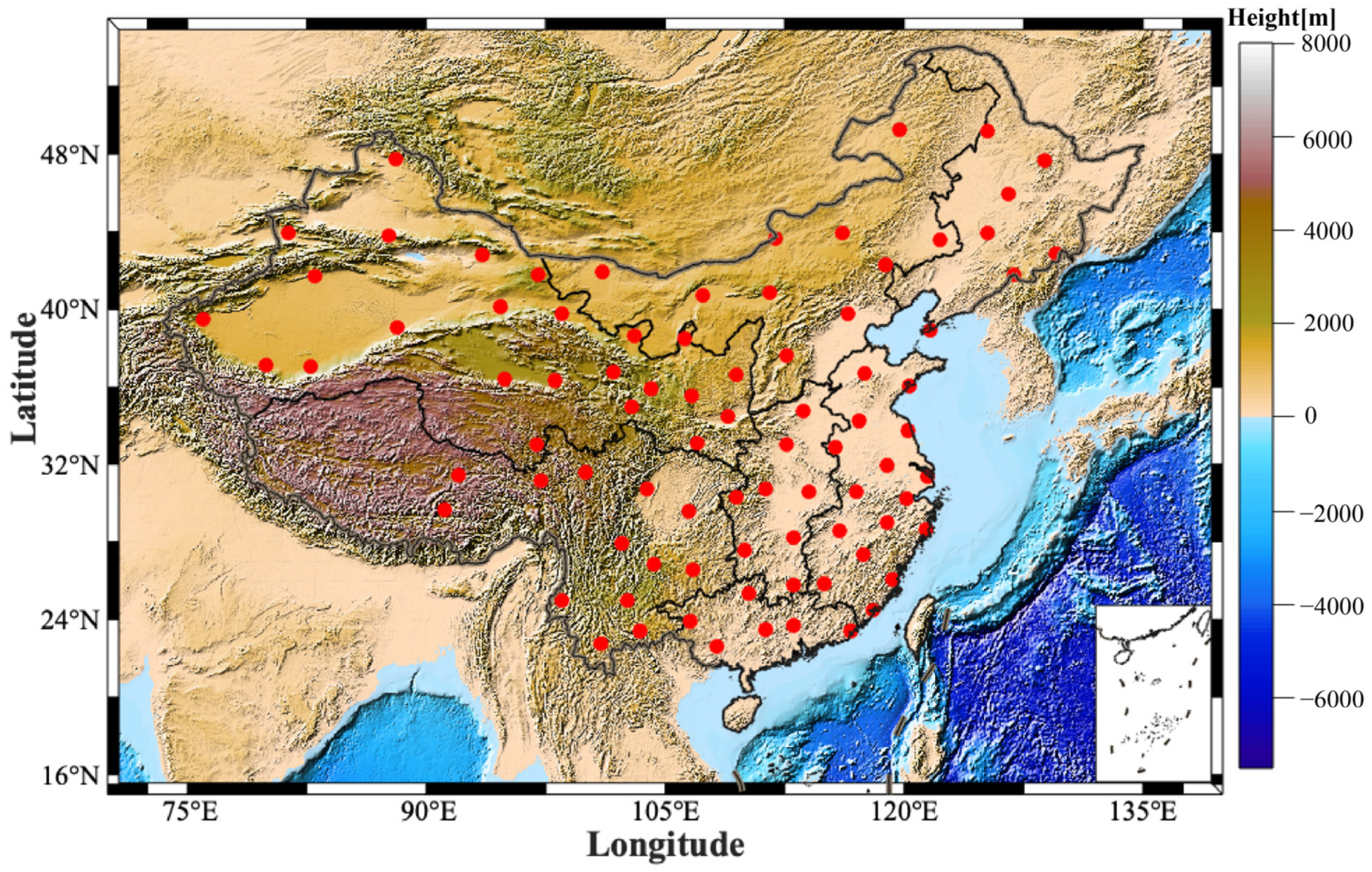
2.1. Experimental Area

The experimental area in this study is mainland China, which is located in China in the range of 16° N–56° N and 72° E–132° E. Figure 1 shows the topography of the experimental area, which indicates that the eastern area has low topography, while the western region has high topography. There are approximately 33% plains and basins in the land area, while mountains, hills, and plateaus are approximately 67%. Moreover, the Qinghai-Tibet Plateau is located in southwestern China. The study area straddles the low- and mid-latitudinal zones. Therefore, the large topographic relief and diverse climate types have resulted in more complex T_m variations, which are challenging to model accurately. In addition, this area has a significantly larger BeiDou/GNSS market. As expected, this market has been going more and more massive since the completion of the Chinese BeiDou navigation network. Therefore, proposing an accurate T_m model in this area can contribute significantly to BeiDou/GNSS meteorology.

2.2. Experimental Data

Radiosonde instruments were collected using radiosonde balloons. The Radiosonde data contained actual measured meteorological information on the relative humidity, temperature, and pressure from the surface to high altitudes, with a time resolution of 12 h. These parameters are used to calculate T_m, which is accurate and usually used as a reference for testing other observations and models [34,35,36]. Therefore, this study used radiosonde data from 84 stations in mainland China from 2015–2018 downloaded free from the Integrated University of Wyoming (http://weather.uwyo.edu/upperair/sounding.html, accessed on 1 March 2021), which contained meteorological data related to pressure, temperature, dew point temperature, and relative humidity at 12 h intervals. These data are used to compute T_m solve the following equation:

$$T_m=\frac{{\displaystyle \mathrm{\int }\frac{e}{T}dz}}{{\displaystyle \mathrm{\int }\frac{e}{T^2}dz}}$$

(1)

where e is the water vapor pressure (hPa) and T is the absolute temperature (K). In practice, because the radiosonde data only contain the pressure level water vapor pressure and temperature, Equation (1) is usually discretized as Equation (2) to calculate T_m.

$$T_m=\frac{{\displaystyle \sum _{i=0}^{i=n-1}\frac{{\overline{e}}_i}{{\overline{T}}_i}(h_{i+1}-h_i)}}{{\displaystyle \sum _{i=0}^{i=n-1}\frac{{\overline{e}}_i}{{\overline{T}}^2{}_i}(h_{i+1}-h_i)}}$$

(2)

$${\overline{e}}_i=\frac{1}{2}\times \left(e_{i+1}{+e}_i\right)$$

(3)

$${\overline{T}}_i=\frac{1}{2}\times \left(T_{i+1}+T_i\right)$$

(4)

where $e_i$ and $T_i$ are the water vapor pressure and absolute temperature of the ith layer, respectively, and $\overline{e_i}$ and $\overline{T_i}$ are the water vapor pressure and mean absolute temperature from layer i to layer i+1, respectively. Radiosonde data do not directly provide water vapor pressure information but relative humidity (RH) and absolute temperature data. Therefore, we calculated the e indirectly from the dew point temperature $T_d$ (°C) and $e_s$ (hPa), which is expressed as follows:

$$e=\frac{RH\times e_{\mathrm{s}}}{100}$$

(5)

$$e_s=6.112\times {10}^{\frac{7.5\times T_d}{T_d+273.3}}$$

(6)

$$T_d=T-273.15$$

(7)

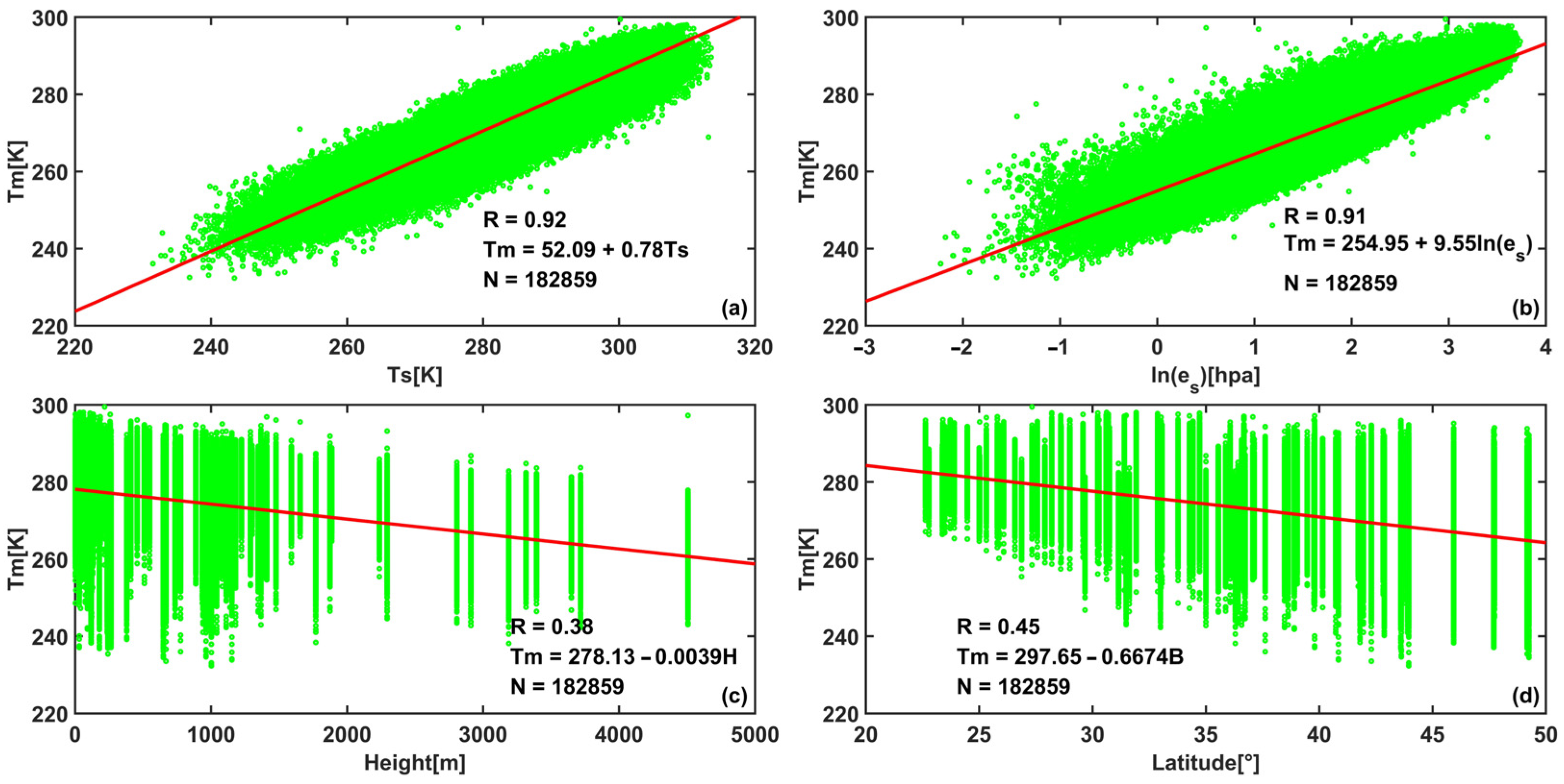
2.3. Tm Empirical Model

As described in Section 1, T_m can be obtained by integration, which has high accuracy but does not allow the user to obtain the T_m value at any position in real time. Therefore, many authors have developed empirical T_m models that consider different factors to achieve real-time conversion from GNSS-ZWD to PWV [22,26,37]. A large part of the T_m model can be represented by Equation (8).

$$T_m=T1(T_s,e_s,H,B)+T2(do{y}_a,do{y}_{\mathrm{s}},do{y}_d)$$

(8)

where $T_s$, $e_s$, $H$, and $B$ correspond to the surface temperature (K), surface water vapor pressure (hPa), height (m), and latitude (°), respectively, and $do{y}_a$, $do{y}_s$, and $do{y}_d$ correspond to the annual, semi-annual, and daily components of the Tm, respectively. In addition, $T1(T_s,e_s,H,B)$ and $T2(do{y}_a,do{y}_{\mathrm{s}},do{y}_d)$ can be denoted as follows:

$$T1(T_s,e_s,H,B)=\left\{\begin{array}{c}{a}_1\times T_s+a_2\\ a_1\times T_s+a_2\times e_s^{a3}+a_4\\ a_1\times T_s+a_2\times e_s^{a3}+a_4\times H+a_5\\ a_1\times T_s+a_2\times e_s^{a3}+a_4\times H+a_5\times B+a_6\end{array}\right\}$$

(9)

$$T2(do{y}_a,do{y}_s,do{y}_d)=\left\{\begin{array}{c}{a}_7\times \mathit{cos}(\frac{doy}{365.25}\times 2\pi )+a_8\times \mathit{sin}(\frac{doy}{365.25}\times 2\pi )+a_9\\ a_7\times \mathit{cos}(\frac{doy}{365.25}\times 4\pi )+a_8\times \mathit{sin}(\frac{doy}{365.25}\times 4\pi )+a_9\\ a_7\times \mathit{cos}(\frac{hod}{24}*2\pi )+a_8\times \mathit{sin}(\frac{hod}{24}*2\pi )+a_9\end{array}\right\}$$

(10)

where $a_1$, $a_2$, $a_3$, $a_4$, $a_5$, $a_6$, $a_7$, $a_8$, and $a_9$ are all unknown coefficients to be determined by the equation.

3. Methods

3.1. GPT3 Model

The GPT3 model is the latest generation of the GPT model [23], which provides empirical T_m values. The GPT3 was established using the 10 years (2001–2010) of monthly mean profiles from the ERA-Interim (37 levels). The topographic model employed by GPT3 is ETOPO5. The accuracy of the GPT3 model reaches 4.2K [31] for estimating T_m globally, and is a widely used model [25,31]. We used the new version of the GPT3 model, whose MATLAB codes and the needed text files can be downloaded from https://vmf.geo.tuwien.ac.at/ accessed on 1 July 2022. When using the GPT3 model to estimate T_m at any station, the model first finds the four grid nodes closest to the test station and calculates the T_m at the four grid nodes. It then interpolates the T_m to the station location through bilinear interpolation. The GPT3 model uses the ellipsoidal height system, while the radiosonde data uses the geopotential height system. It is necessary to convert the geopotential height of radiosonde data to an ellipsoidal height system. We employed the Earth Gravity Model 2008 (EGM 2008) model to realize the unification of the height system [38]. The variation characteristics of meteorological parameters over time for the GPT3 model are characterized by Equation (11). The spatial resolution of the meteorological parameters obtained using the GPT3 model was classified into 5° × 5°, and 1° × 1°, according to the grid size.

$$\begin{array}{c}r(t)=A_0+A_1\mathit{cos}(\frac{doy}{365.25}2\pi )+B_1\mathit{sin}(\frac{doy}{365.25}2\pi )\\ +A_2\mathit{cos}(\frac{doy}{365.25}4\pi )+B_2\mathit{sin}(\frac{doy}{365.25}4\pi )\end{array}$$

(11)

where r(t) indicates T_m, doy indicates the annual accumulation days, $A_0$ indicates the annual average, $A_1$ and $B_1$ are the annual cycle coefficients, and $A_2$ and $B_2$ are the semi-annual cycle coefficients.

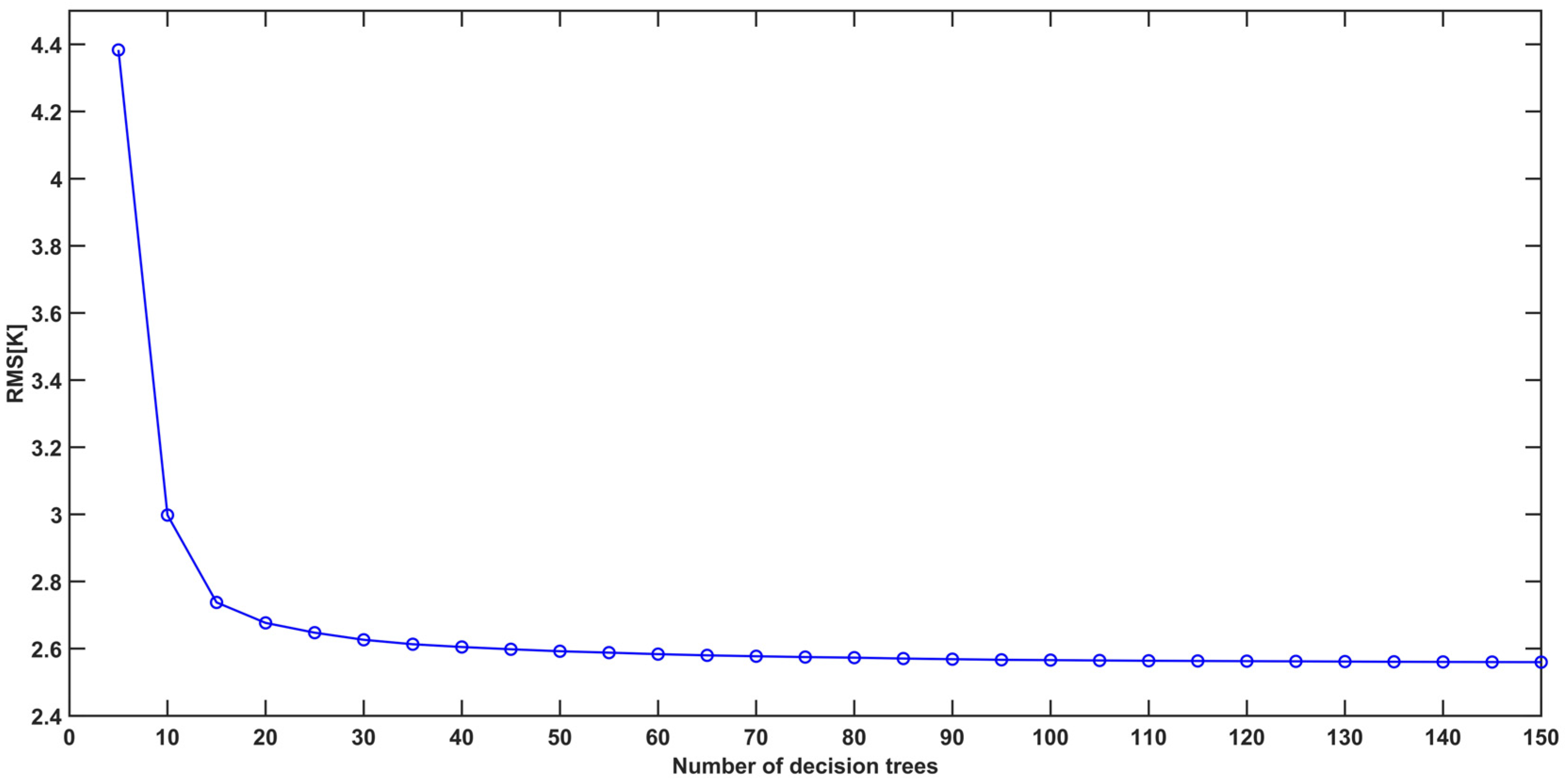
3.2. Modeling with the Random Forest Regression Algorithm Model

The random forest (RF) model was first proposed as a machine learning algorithm by Leo Breiman and Adele Cutler in 2001 [39]. RF is a machine-learning algorithm that can map the nonlinear relationship between diffident variables with good interpretability and good prediction ability. It solves classification or regression problems by building a large number of unpruned regression trees based on classification or regression algorithms.

In this study, we mainly used the RF regression algorithm, which uses the bootstrap aggregation method to randomly draw multiple samples from the original data to build a regression tree, and it finally takes the average of all regression trees as the final prediction result. During the construction of the regression tree, the split point of the regression tree was determined by minimizing the regression error, where the regression error was the weighted sum of the regression errors of each subset, as shown in Equations (12) and (13).

$$K=\frac{M_L}{M}*K(B_L)+\frac{M_R}{M}*K(B_R)$$

(12)

$$M(B)=\frac{{\displaystyle \sum _{i=1}^M{(y_i-\overline{y})}^2}}{M}$$

(13)

where $K(B)$ is the regression error, $K(B_L)$ and $K(B_R)$ denote the regression error of the left and right subsets, respectively, and $M_L$, $M_R$ and $M$ is the number of left subsets, right subsets, and total samples.

The RF_Tm model was used, as shown in Figure 2. We found from the correlation analysis in Section 3.4 that surface temperature, surface water vapor pressure, height, and latitude were the critical factors affecting the accuracy of T_m. Therefore, we used T_s, e_s, latitude (B), height (H), and GPT3-Tm of 84 radiosonde stations from 2015–2017 as the input values of the RF_Tm model. It is well known that T_m has seasonal variations, so time was also employed in the input value. Note that the “Time” in Figure 2 denotes the day of the year plus the hour of the day divided by 24. Then, the T_m at the location of the radiosonde stations was obtained by integration as the output values of the RF_Tm model, and trained to obtain the RF_Tm model.

3.3. Model Evaluation Index

To test the accuracy of the RF_Tm model established in this study, we used the T_m of 84 radiosonde stations of the China region in 2018 as the reference values, and the mean bias (Bias) and root mean square (RMS) as the accuracy indicators. Bias and RMS were calculated as follows:

$$Bias=\frac{1}{N}\times {\displaystyle \sum _{t=1}^N(X_t-P_t)}$$

(14)

$$RMS=\sqrt{\frac{1}{N}\times {{\displaystyle \sum _{t=1}^N(X_t-P_t)}}^2}$$

(15)

where N denotes the number of predicted samples and $X_t$ and $P_t$ are the true value of the Tm and the predicted value of the model, respectively.

3.4. RF_Tm Model Establishment

Two important parameters are included in the random forest: the number of single regression tree features and the number of regression trees constructed. To select tree features, we employed the Pearson correlation coefficient [40] of Equation (16) for the correlation analysis of the T_m with other parameters, such as T_s, e_s, height, and latitude.

$$R=\frac{{\displaystyle \sum _{i=1}^n(X_i-\overline{X}})\times (Y_i-\overline{Y})}{\sqrt{{\displaystyle \sum _{i=1}^n{(X_i-\overline{X})}^2}}\times \sqrt{{\displaystyle \sum _{i=1}^n{(Y_i-\overline{Y})}^2}}}$$

(16)

where n denotes the number of samples, and X and Y represent two different variables.

The correlation analysis results are presented in Figure 3. Note that the correlation follows the criteria: r ≥ 0.81–1.0 excellent, 0.61–0.80 very good, 0.41–0.60 good, 0.21–0.40 fair, and 0.0–0.20 poor. Figure 3a,b shows that the correlation coefficients of the T_m with T_s and ln(e_s) in mainland China are 0.92 and 0.91, respectively, indicating an excellent correlation. Figure 3c,d shows that the correlation coefficients of height and latitude with T_m are 0.38 and 0.45, signifying a fair and good correlation, respectively. In terms of the degree of correlation, T_s, e_s, height, and latitude were chosen as tree features for T_m modelling.

We found that T_s and ln(e_s) show an excellent linear correlation with T_m, while the Pearson linear correlation between T_m and height and T_m and latitude were fair and good. Moreover, Sun et al. [27] revealed that the input of empirical values could improve the accuracy of machine learning models. The surface temperature, surface water vapor pressure, time, height, latitude, and GPT3-T_m provided by the radiosonde station were used as features of the single regression tree. After determining the single regression tree features, we used the different features selected as the input values and the radiosonde station Tm as the output values to train a new T_m model (RF_Tm).

The fitting accuracy of the RF_Tm model was affected by the number of regression trees. The metric for selecting the number of regressions in this paper was the minimum RMS for out-of-bag observations in the training data using the trained bagger B. Therefore, a step of five was used to set the number of regression trees as 5–150 to train the RF_Tm, and then the RMS for out-of-bag observations in the training data was statistically calculated. The statistical results are shown in Figure 4, which indicates that the RMS continues to decrease as the number of regression trees increases. When the number of regression trees reaches approximately 100, the RMS stabilizes at around 2.6 K. After the number of regression trees exceeded 100, the RMS remained almost unchanged. Therefore, we selected 100 regression trees to build the final model (RF_Tm).

4. Results and Analysis

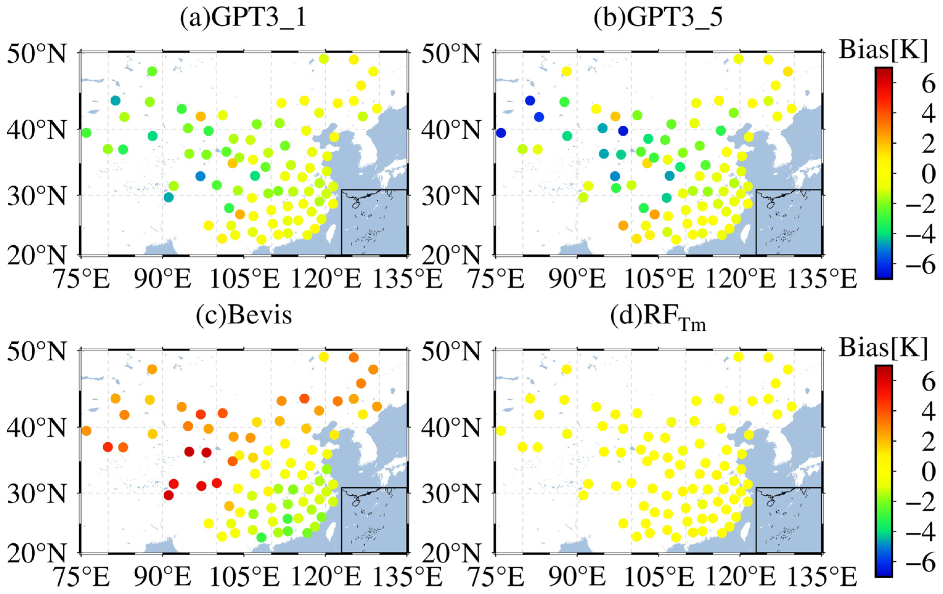
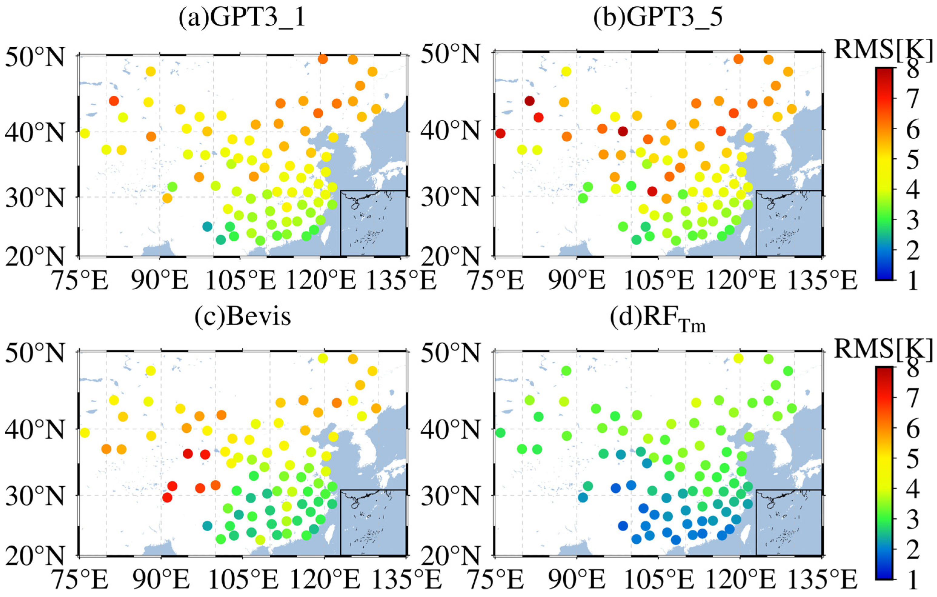
4.1. Global Accuracies

To comprehensively evaluate the applicability of the RF_Tm model, we used the 2018 radiosonde T_m not involved in the modeling as the reference and statistically analyzed the Bias and RMS of the RF_Tm, Bevis, GPT3-1 (1° × 1°), and GPT3-5 models (5° × 5°). The statistical results are shown in

Table 1. Overall accuracy of the different models in 2018.

Model/Accuracy		Bevis	RFTm	GPT3-1	GPT3-5
RMS	Max	7.32	4.08	7.30	7.97
	Min	2.32	1.68	2.31	2.70
	Ave	4.45	2.87	4.69	5.17
Bias	Max	6.45	0.80	2.20	2.52
	Min	−2.96	−0.54	−6.76	−7.21
	Ave	1.12	0.13	−1.22	−1.55

.

Table 1 shows that compared with the Bevis, GPT3-1, and GPT3-5 models, the maximum, minimum, and average of Bias and RMS of the RF_Tm were greatly smaller and reached 0.13 K and 2.87 K, respectively. The RMS of the RF_Tm was reduced by 35.5%, 38.8%, and 44.7% compared with that of the Bevis, GPT3-1, and GPT3-5 models, respectively. These results indicate that the overall accuracy of the RF_Tm was better than that of the Bevis and GPT3 models in mainland China. The RMS of the maximum, minimum, and average of the Bevis and GPT3 models were similar, although the maximum and minimum Bias values of the Bevis, GPT3-1, and GPT3-5 models differed significantly, with annual average values of 1.12, -1.22 K, and -1.55 K, respectively. Moreover, the overall accuracy of the GPT3-1/5 models and the Bevis models was not very different.

Because China has a large area, the adaptability of the model has to be analyzed in different regions of China. The Bias and RMS were calculated for different models at 84 stations, and the results are shown in Figure 5 and Figure 6.

Figure 5a,b shows that the Bias of the GPT3-1 and GPT3-5 models was distributed between −4 K and 0 K in mainland China, and the absolute value of the Bias was greater than 4 K in the western region of China, which may be attributed to the higher terrain in the western region. As shown in Figure 5c, the distribution of Bias for the Bevis model in the southern region of China was between −4 K and 0 K, while that in the northern region of China was between 0 K and 7 K. These discrepancies are likely due to the more drastic variation in the T_m in the middle and high latitudes [19]. More interestingly, contrary to Bevis’s Tm estimation showing positive and negative bias values, the GPT3’s T_m prediction is systematically bigger than the measured T_m in mainland China, which is mainly due to the complex terrain of the study area, as the GPT3 model does not consider the impact in T_m from height differences between the grid sites and the test sites. Figure 5d indicates that the Bias of the RF_Tm was concentrated around 0 K in different regions of China, indicating that the adaptation of the RF_Tm in different regions of China was better than that of Bevis, GPT3-1, and GPT3-5.

As shown in Figure 6, the RMS of the RF_Tm in the southern region of China was distributed between 2 K and 3 K, while that of the GPT3-5, GPT3-1, and Bevis models ranged from 3–4 K. The RMS of the RF_Tm was reduced by approximately 1 K compared with that of the GPT3-1, GPT3-5, and Bevis models. In northern China, the RMS of the RF_Tm ranged from 3 K to 4 K, and that of GPT3-1 ranged from 5 K to 6 K. The RMS of GPT3-5 was slightly worse than that of GPT3-1. The RMS of Bevis was distributed around 5 K, which is superior to that of GPT3-1 and GPT3-5, whereas the RMS of the RF_Tm was optimal. Generally, RF_Tm was more stable than Bevis, GPT3-1, and GPT3-5 in different regions of the study area.

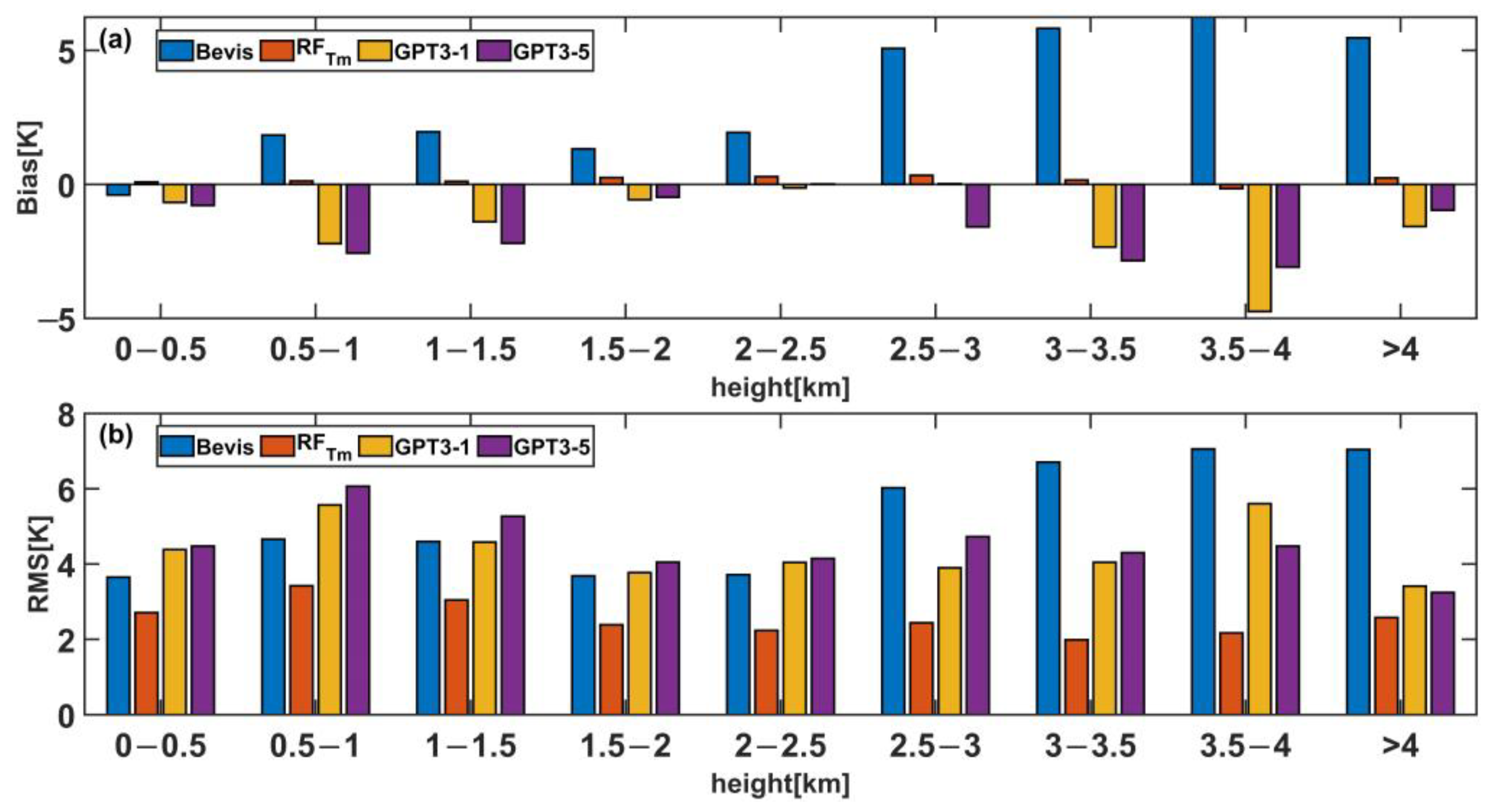
4.2. Accuracies in Different Heights

Height is a key factor that affects the T_m [13,22]. To analyze the adaptability of different models at different heights, we statistically analyzed the Bias and RMS of the Bevis, RF_Tm, GPT3-1, and GPT3-5 models from 0 km to 4.5 km at intervals of 500 m. The results are shown in Figure 7 and

Table 2. RMS of different models at different heights of the T_m in 2018.

Height	RMS[K]
	Bevis	RFTm	GPT3-1	GPT3-5
0–500	3.65	2.71	4.38	4.48
500–1000	4.66	3.42	5.57	6.07
1000–1500	4.60	3.05	4.58	5.27
1500–2000	3.69	2.39	3.77	4.05
2000–2500	3.72	2.24	4.04	4.15
2500–3000	6.02	2.44	3.90	4.73
3000–3500	6.71	1.99	4.05	4.30
3500–4000	7.06	2.17	5.60	4.48
>4000	7.04	2.58	3.41	3.24

.

As shown in Figure 7 and Table 2, the Bias of the Bevis model was overall positive at different heights. Both the Bias and RMS of the Bevis model showed an increasing trend with higher height, which may be attributed to the fact that the Bevis model has not corrected for T_m in the height direction. The GPT3-1 and GPT3-5 models both had negative Bias values at different heights. According to Figure 7 and

Table 3. Bias of different models at different heights of the T_m in 2018.

Height	Bias[K]
	Bevis	RFTm	GPT3-1	GPT3-5
0–500	−0.39	0.09	−0.67	−0.78
500–1000	1.84	0.12	−2.21	−2.56
1000–1500	1.96	0.11	−1.40	−2.20
1500–2000	1.32	0.25	−0.57	−0.48
2000–2500	1.93	0.29	−0.13	0.02
2500–3000	5.08	0.34	0.02	−1.59
3000–3500	5.82	0.16	−2.34	−2.84
3500–4000	6.24	-0.16	−4.75	−3.08
>4000	5.47	0.24	−1.57	−0.97

, the GPT3-1 and GPT3-5 models’ Bias was concentrated at −5 K to 0 K, while the Bevis model Bias was distributed at 0 K to 5 K. The fluctuation range of Bias for the Bevis model was approximately opposite to the fluctuation range of the GPT3-1 and GPT3-5 models. The GPT3-1 and GPT3-5 models showed large fluctuations of Bias up and down with the increase in height, and the Bias was concentrated from −1 K to 0 K in 0–500 m and 1500–3000 m and from −5 K to −1 K in 500–1500 m and above 3000 m. For the RF_Tm model, the Bias was distributed around 0 K at different heights, and the RMS values were all less than 3 K. This finding indicates that the RF_Tm has better applicability to height than Bevis, GPT3-1, and GPT3-5. Moreover, the RF_Tm considers the effect of height on the T_m, which further verifies the rationality of using height as a model factor in this study.

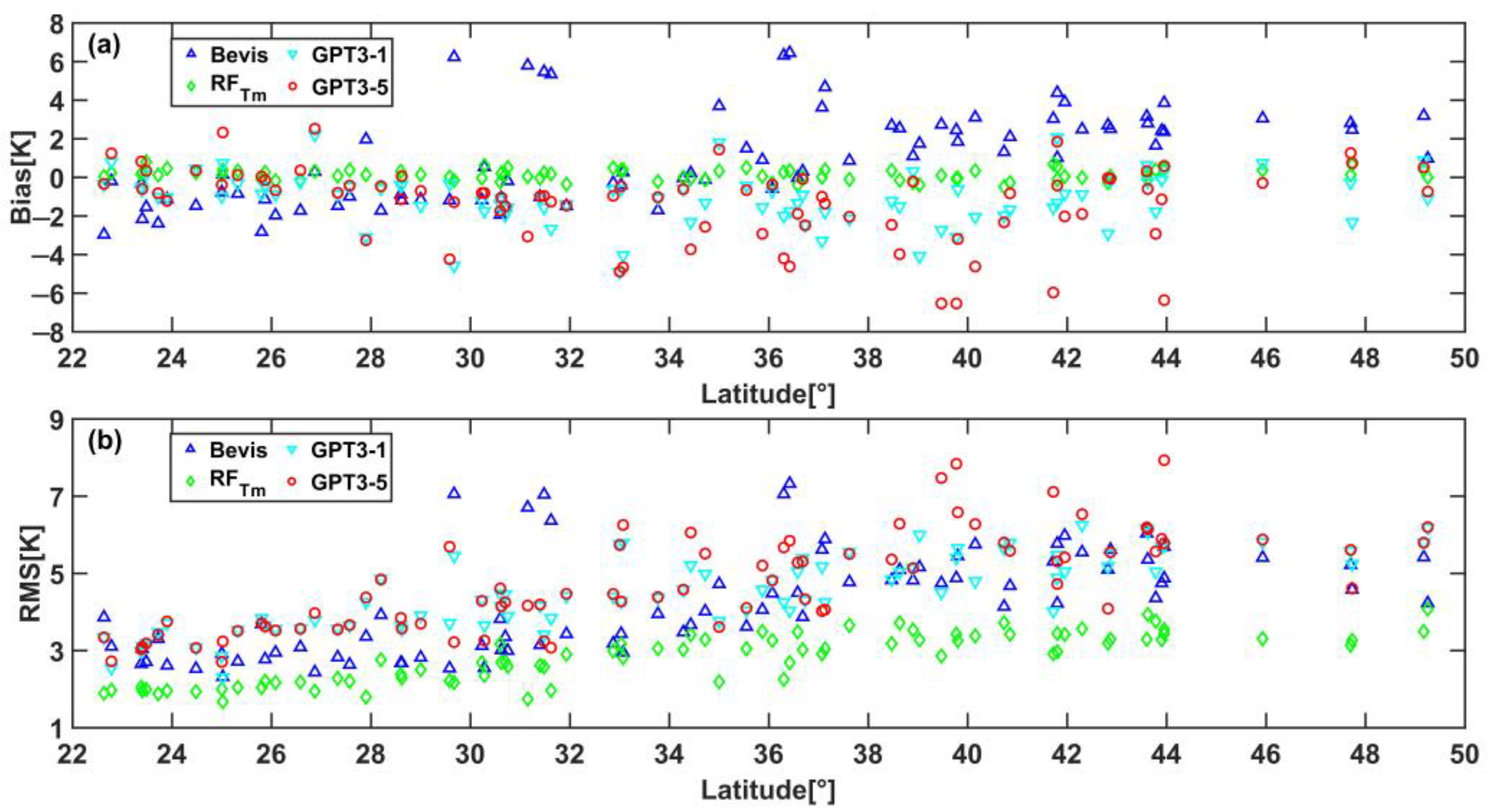
4.3. Accuracies in Different Latitudes

The variation of T_m with latitude is more obvious [27,34]. Therefore, we computed the Bias and RMS of T_m for 2018 predicted by different models in latitude direction, and the results are shown in Figure 8.

As shown in Figure 8a, the Bias of the Bevis model presented negative values in latitudes lower than 30°, while the Bias of RF_Tm, GPT3-1, and GPT3-5 models were concentrated around 0 K. On latitudes larger than 30°, the Bias of Bevis, GPT3-1, and GPT3-5 models ranged from 0 K to 8 K, −6 K to 2 K, and −8 K to 2 K, respectively. The Bias range of the GPT3-5 model was larger than GPT3-1. The Bias of RF_Tm was concentrated around 0 K. The Bias of the RF_Tm model was concentrated at around 0K. However, when the latitude was greater than 40°, Bias was greater than 0 K. This phenomenon may be because the seasonal variation of T_m was larger at high latitudes [19], which posed more difficulties for T_m modeling and resulted in a larger Bias for T_m models. Even so, its corresponding RMS is within 3 K, which is significantly better than the Bevis and GPT3 models. These results suggest that the RF_Tm model can better capture the variation of T_m in the latitudinal direction than the Bevis, GPT3-1, and GPT3-5 models. In Figure 8b, the RMS of the Bevis, RF_Tm, GPT3-1, and GPT3-5 models tended to become larger with rising latitude, but the RMS of RF_Tm was concentrated within 3 K. The RMS of RF_Tm with increasing latitude was notably lower than that of Bevis, GPT3-1, and GPT3-5, indicating that the adaptation of RF_Tm to latitude changes was better than that of Bevis, GPT3-1, and GPT3-5. Generally, the RF_Tm model has lower Bias and RMS than the Bevis, GPT3-1, and GPT3-5 models in different regions. These also imply that RF_Tm has better stability and adaptability than Bevis, GPT3-1, and GPT3-5 at various latitudes.

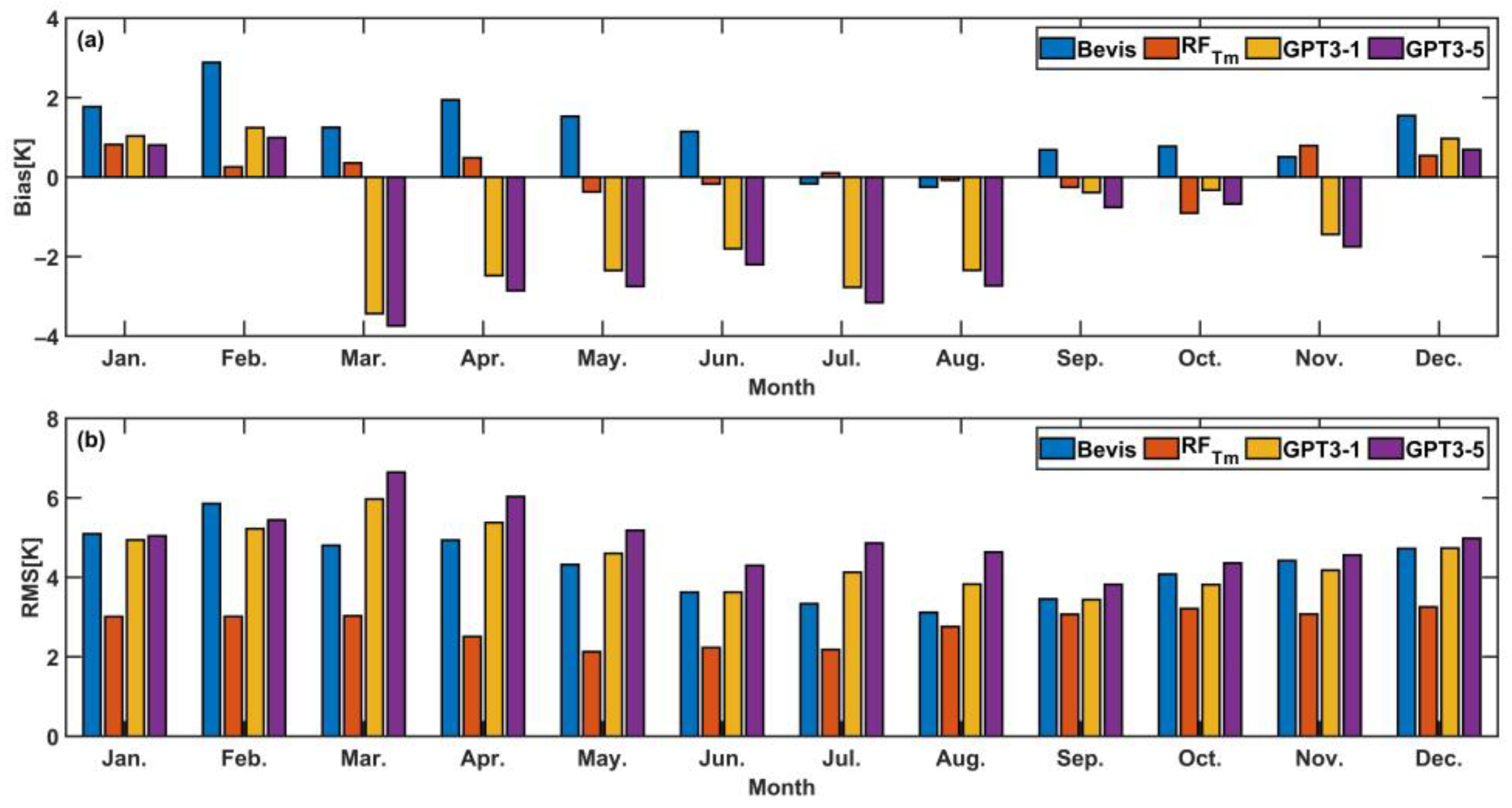
4.4. Accuracies in Different Time Variations

To further investigate the relationship between the models and time, we computed the Bias and RMS from the Bevis, GPT3-1, GPT3-5, and RF_Tm models in 2018 with a temporal resolution of 12 h, respectively. The results are shown in Figure 9.

Figure 9, Figure 10 and Figure 11 show the daily, monthly, and quarterly average Bias and RMS variations for the four models, respectively. As illustrated in Figure 9, Figure 10 and Figure 11, the Bias of the RF_Tm model fluctuated above and below 0 K, and the RMS of the RF_Tm model ranged between 2 K and 4 K. The RF_Tm model showed better RMS and Bias than the Bevis, GPT3-1, and GPT3-5 models for different months and seasons, and there was no apparent seasonal variation in Bias and RMS. The reason for this phenomenon might be that RF_Tm model added a time factor in the modeling, which somewhat weakened the influence of seasonal variation on the model accuracy. Bias and RMS of the Bevis, GPT3-1, and GPT3-5 models were larger in winter and spring but relatively lower in summer and autumn. The RMS of the GPT3-1 and GPT3-5 models fluctuated at around 5 K. The variation of Bias with time was mainly distributed between −10 K and 0 K, and extremely few of them were distributed between 0 K and 6 K, indicating that the GPT3-1 and GPT3-5 models might have negative deviations overall. The RMS of the Bevis model fluctuated around 5 K, which was consistent with that of the GPT3-1 and GPT3-5 models, but the overall Bevis model Bias ranged from 0 K to 6 K, denoting that the Bevis model showed an overall positive deviation in mainland China. Overall, RF_Tm outperforms at different times than Bevis, GPT3-1, and GPT3-5.

5. Conclusions

We proposed a weighted mean temperature model (RF_Tm) based on a random forest with GPT3-T_m, surface water vapor pressure, surface temperature, height, latitude, and time as input parameters in the paper, and tested the accuracy of RF_Tm in the Chinese region. The results indicated that: The RF_Tm model achieved better accuracy in mainland China as a whole, and its annual average Bias and RMS were 0.13 K and 2.87 K. Compared with the Bevis model, GPT3-1 model, and GPT3-5 model, the annual average RMS of RF_Tm model were reduced by 35.5%, 38.8%, and 44.7%, respectively. The overall accuracy of RF_Tm model has been significantly superior to that of the Bevis model and the GPT3-1 and GPT3-5 models. The RF_Tm model had better accuracy than the Bevis model, GPT3-1 model, and GPT3-5 model for different latitudes and heights, and it captured the change of T_m with height and latitude more effectively than the Bevis model, GPT3-1 model, and the GPT3-5 model. The RF_Tm model could better perceive the change of T_m with time in comparison to the Bevis model, the GPT3-1 model, and the GPT3-5 model.

Comprehensive validations indicate that the RF_Tm model based on RF outperformes the Bevis model and GPT3 model in mainland China, and the accuracy is more stable in different spatiotemporal intervals. Therefore, the proposed model can be implemented for the relevant application of GNSS meteorology in China. However, the proposed model only supports regional T_m estimation and needs in situ measured meteorological. In future research, we hope to develop a global machine learning-based model for estimating T_m based only on geographical and temporal information.

References

1. Karabatić, A.; Weber, R.; Haiden, T. Near Real-Time Estimation of Tropospheric Water Vapour Content from Ground Based GNSS Data and Its Potential Contribution to Weather Now-Casting in Austria. Adv. Space Res. 2011, 47, 1691–1703. [Google Scholar] [CrossRef]
2. Vázquez, B.G.E.; Grejner-Brzezinska, D.A. GPS-PWV Estimation and Validation with Radiosonde Data and Numerical Weather Prediction Model in Antarctica. GPS Solut. 2013, 17, 29–39. [Google Scholar] [CrossRef]
3. Xiong, Z.; Sang, J.; Sun, X.; Zhang, B.; Li, J. Comparisons of Performance Using Data Assimilation and Data Fusion Approaches in Acquiring Precipitable Water Vapor: A Case Study of a Western United States of America Area. Water 2020, 12, 2943. [Google Scholar] [CrossRef]
4. Chen, B.; Liu, Z. A Comprehensive Evaluation and Analysis of the Performance of Multiple Tropospheric Models in China Region. IEEE Trans. Geosci. Remote Sens. 2016, 54, 663–678. [Google Scholar] [CrossRef]
5. Davis, J.L.; Herring, T.A.; Shapiro, I.I.; Rogers, A.E.E.; Elgered, G. Geodesy by Radio Interferometry: Effects of Atmospheric Modeling Errors on Estimates of Baseline Length. Radio Sci. 1985, 20, 1593–1607. [Google Scholar] [CrossRef]
6. Askne, J.; Nordius, H. Estimation of Tropospheric Delay for Microwaves from Surface Weather Data. Radio Sci. 1987, 22, 379–386. [Google Scholar] [CrossRef]
7. Zhao, Q.; Liu, Y.; Yao, W.; Yao, Y. Hourly Rainfall Forecast Model Using Supervised Learning Algorithm. IEEE Trans. Geosci. Remote Sens. 2022, 60, 1–9. [Google Scholar] [CrossRef]
8. Baldysz, Z.; Nykiel, G. Improved Empirical Coefficients for Estimating Water Vapor Weighted Mean Temperature over Europe for GNSS Applications. Remote Sens. 2019, 14, 1995. [Google Scholar] [CrossRef]
9. Bevis, M.; Businger, S.; Chiswell, S.; Herring, T.A.; Anthes, R.A.; Rocken, C.; Ware, R.H. GPS Meteorology: Mapping Zenith Wet Delays onto Precipitable Water. J. Appl. Meteorol. Climatol. 1994, 33, 379–386. [Google Scholar] [CrossRef]
10. Geng, Y.; Bao, Z. Establishment and Analysis of Global Gridded Tm−Ts Relationship Model. Geod. Geodyn. 2016, 7, 101–107. [Google Scholar] [CrossRef] [Green Version]
11. Mircheva, B.; Tsekov, M.; Meyer, U.; Guerova, G. Anomalies of Hydrological Cycle Components during the 2007 Heat Wave in Bulgaria. J. Atmos. Sol. Terr. Phys. 2017, 165–166, 1–9. [Google Scholar] [CrossRef]
12. Isioye, O.A.; Combrinck, L.; Botai, J. Modelling Weighted Mean Temperature in the West African Region: Implications for GNSS Meteorology. Meteorol. Appl. 2016, 23, 614–632. [Google Scholar] [CrossRef]
13. Li, L.; Wu, S.; Wang, X.; Tian, Y.; He, C.; Zhang, K. Seasonal Multifactor Modelling of Weighted-Mean Temperature for Ground-Based GNSS Meteorology in Hunan, China. Adv. Meteorol. 2017, 14, 3782687. [Google Scholar] [CrossRef]
14. Peng, J.; Ye, S.; Yinhao, L.; Liu, Y.; Chen, D.; Wu, Y. Development of Time-Varying Global Gridded Ts-Tm Model for Precise GPS-PWV Retrieval. Atmos. Meas. Tech. Discuss. 2018, 12, 1233–1249. [Google Scholar] [CrossRef]
15. Yao, Y.; Bao, Z.; Xu, C.; Yan, F. Improved One/Multi-Parameter Models That Consider Seasonal and Geographic Variations for Estimating Weighted Mean Temperature in Ground-Based GPS Meteorology. J. Geod. 2014, 88, 273–282. [Google Scholar] [CrossRef]
16. Junyu, L.; Bao, Z.; Yao, Y.; Liu, L.; Zhangyu, S.; Yan, X. A Refined Regional Model for Estimating Pressure, Temperature, and Water Vapor Pressure for Geodetic Applications in China. Remote Sens. 2020, 12, 1713. [Google Scholar] [CrossRef]
17. Yao, Y.; Zhu, S.; Yue, S. A Globally Applicable, Season-Specific Model for Estimating the Weighted Mean Temperature of the Atmosphere. J. Geod. 2012, 86, 1125–1135. [Google Scholar] [CrossRef]
18. He, C.; Wu, S.; Wang, X.; Hu, A.; Wang, Q.; Zhang, K. A New Voxel-Based Model for the Determination of Atmospheric Weighted Mean Temperature in GPS Atmospheric Sounding. Atmos. Meas. Tech. 2017, 10, 2045–2060. [Google Scholar] [CrossRef]
19. Sun, Z.; Zhang, B.; Yao, Y. A Global Model for Estimating Tropospheric Delay and Weighted Mean Temperature Developed with Atmospheric Reanalysis Data from 1979 to 2017. Remote Sens. 2019, 11, 1893. [Google Scholar] [CrossRef]
20. Li, Q.; Yuan, L.; Chen, P.; Zhongshan, J. Global Grid-Based Tm Model with Vertical Adjustment for GNSS Precipitable Water Retrieval. GPS Solut. 2020, 24, 73. [Google Scholar] [CrossRef]
21. Boehm, J.; Heinkelmann, R.; Schuh, H. Short Note: A Global Model of Pressure and Temperature for Geodetic Applications. J. Geod. 2007, 81, 679–683. [Google Scholar] [CrossRef]
22. Böhm, J.; Möller, G.; Schindelegger, M.; Pain, G.; Weber, R. Development of an Improved Empirical Model for Slant Delays in the Troposphere (GPT2w). GPS Solut. 2015, 19, 433–441. [Google Scholar] [CrossRef]
23. Landskron, D.; Böhm, J. VMF3/GPT3: Refined Discrete and Empirical Troposphere Mapping Functions. J. Geod. 2018, 92, 349–360. [Google Scholar] [CrossRef]
24. Zhu, M.; Yu, X.; Sun, W. A Coalescent Grid Model of Weighted Mean Temperature for China Region Based on Feedforward Neural Network Algorithm. GPS Solut. 2022, 26, 70. [Google Scholar] [CrossRef]
25. Yang, F.; Guo, J.; Meng, X.; Shi, J.; Zhang, D.; Zhao, Y. An Improved Weighted Mean Temperature (Tm) Model Based on GPT2w with Tm Lapse Rate. GPS Solut. 2020, 24, 46. [Google Scholar] [CrossRef]
26. Huang, L.; Jiang, W.-P.; Liu, L.; Chen, H.; Ye, S. A New Global Grid Model for the Determination of Atmospheric Weighted Mean Temperature in GPS Precipitable Water Vapor. J. Geod. 2018, 93, 159–176. [Google Scholar] [CrossRef]
27. Sun, Z.; Zhang, B.; Yao, Y. Improving the Estimation of Weighted Mean Temperature in China Using Machine Learning Methods. Remote Sens. 2021, 13, 1016. [Google Scholar] [CrossRef]
28. Umakanth, N.; Satyanarayana, G.C.; Simon, B.; Rao, M.C.; Babu, N.R. Long-Term Analysis of Thunderstorm-Related Parameters over Visakhapatnam and Machilipatnam, India. Acta Geophys. 2020, 68, 921–932. [Google Scholar] [CrossRef]
29. Ding, W.; Qie, X. Prediction of Air Pollutant Concentrations via RANDOM Forest Regressor Coupled with Uncertainty Analysis—A Case Study in Ningxia. Atmosphere 2022, 13, 960. [Google Scholar] [CrossRef]
30. Tran, T.T.K.; Lee, T.; Kim, J.-S. Increasing Neurons or Deepening Layers in Forecasting Maximum Temperature Time Series? Atmosphere 2020, 11, 1072. [Google Scholar] [CrossRef]
31. Ding, M. A Neural Network Model for Predicting Weighted Mean Temperature. J. Geod. 2018, 92, 1187–1198. [Google Scholar] [CrossRef]
32. Long, F.; Hu, W.; Dong, Y.; Wang, J. Neural Network-Based Models for Estimating Weighted Mean Temperature in China and Adjacent Areas. Atmosphere 2021, 12, 169. [Google Scholar] [CrossRef]
33. Yang, L.; Chang, G.; Qian, N.; Gao, J. Improved Atmospheric Weighted Mean Temperature Modeling Using Sparse Kernel Learning. GPS Solut. 2021, 25, 28. [Google Scholar] [CrossRef]
34. Wang, S.; Xu, T.; Nie, W.; Wang, J.; Xu, G. Establishment of Atmospheric Weighted Mean Temperature Model in the Polar Regions. Adv. Space Res. 2019, 65, 518–528. [Google Scholar] [CrossRef]
35. Zhang, H.; Yuan, Y.; Li, W.; Ou, J.; Li, Y.; Zhang, B. GPS PPP-derived Precipitable Water Vapor Retrieval Based on Tm/Ps from Multiple Sources of Meteorological Datasets in China. J. Geophys. Res. Atmos. 2017, 122, 4165–4183. [Google Scholar] [CrossRef]
36. Li, T.; Wang, L.; Chen, R.; Fu, W.; Xu, B.; Jiang, P.; Liu, J.; Zhou, H.; Han, Y. Refining the Empirical Global Pressure and Temperature Model with the ERA5 Reanalysis and Radiosonde Data. J. Geod. 2021, 95, 31. [Google Scholar] [CrossRef]
37. Zhao, Q.; Yao, Y.; Yao, W.; Zhang, S. GNSS-Derived PWV and Comparison with Radiosonde and ECMWF ERA-Interim Data over Mainland China. J. Atmos. Sol. Terr. Phys. 2019, 182, 85–92. [Google Scholar] [CrossRef]
38. Huang, L.; Guo, L.; Liu, L.; Chen, H.; Chen, J.; Xie, S. Evaluation of the ZWD/ZTD Values Derived from MERRA-2 Global Reanalysis Products Using GNSS Observations and Radiosonde Data. Sensors 2020, 20, 6440. [Google Scholar] [CrossRef]
39. Breiman, L. Random Forests. Mach. Learn. 2001, 45, 5–32. [Google Scholar] [CrossRef]
40. Rahman, M.; Zhang, Q. Comparison among Pearson Correlation Coefficient Tests. Far East Journal of Mathematical Sciences (FJMS). 2015, 99, 237–255. [Google Scholar] [CrossRef]
Figure 1. Distribution of 84 radiosonde stations in mainland China.
Atmosphere 13 01368 g001
Figure 2. Flow chart of the random forest method.
Atmosphere 13 01368 g002
Figure 3. Correlation analysis diagram of the Tm and Ts, ln(es), height, and latitude, where (a) is the correlation analysis diagram of Tm and Ts where (b) is the correlation analysis diagram of Tm and ln(es) where (c) is the correlation analysis diagram of Tm and height, and (d) is the correlation analysis diagram of Tm and latitude.
Atmosphere 13 01368 g003
Figure 4. Fitting accuracy of the RFTm model with different numbers of regression trees.
Atmosphere 13 01368 g004
Figure 5. Bias variation diagram for Tm from the different models in 2018, where (a) is the Bias changes of GPT3_1 Tm where (b) is the Bias changes of GPT3_5 Tm where (c) is the Bias changes of Bevis Tm where (d) is the Bias changes of RFTm Tm.
Atmosphere 13 01368 g005
Figure 6. RMS variation diagram for Tm from the different models in 2018, where (a) is the RMS changes of GPT3_1 Tm where (b) is the RMS changes of GPT3_5 Tm where (c) is the RMS changes of Bevis Tm where (d) is the RMS changes of RFTm Tm.
Atmosphere 13 01368 g006
Figure 7. Variation of the Tm with height in 2018 for the different models, where (a) is the variation of the Bias in the height direction for Tm predicted by different models in 2018, and (b) is the variation of RMS in the height direction for Tm predicted by different models in 2018.
Atmosphere 13 01368 g007
Figure 8. The latitude variation of Tm predicted by different models in 2018, where (a) is the variation of Bias in the latitudinal direction for Tm predicted by different models in 2018, and (b) is the variation of RMS in the latitudinal direction for Tm predicted by different models in 2018.
Atmosphere 13 01368 g008
Figure 9. Bias and RMS of different models Tm in 2018, where (a) is the Bias of different models Tm in 2018, and (b) is the RMS of different models Tm in 2018.
Atmosphere 13 01368 g009
Figure 10. Monthly average Bias and RMS of different models Tm in 2018, where (a) is the monthly average Bias changes of different models Tm in 2018, and (b) is the monthly average RMS changes of different models Tm in 2018.
Atmosphere 13 01368 g010
Figure 11. Bias and RMS of different models Tm over the four seasons in 2018, where (a) is the Bias of different models Tm over the four seasons in 2018, and (b) is the RMS of different models Tm over the four seasons in 2018.
Atmosphere 13 01368 g011