
The European Standard EN 15757 Concerning Specifications for Relative Humidity: Suggested Improvements for Its Revision


Abstract
:1. Introduction
2. Data and Methods
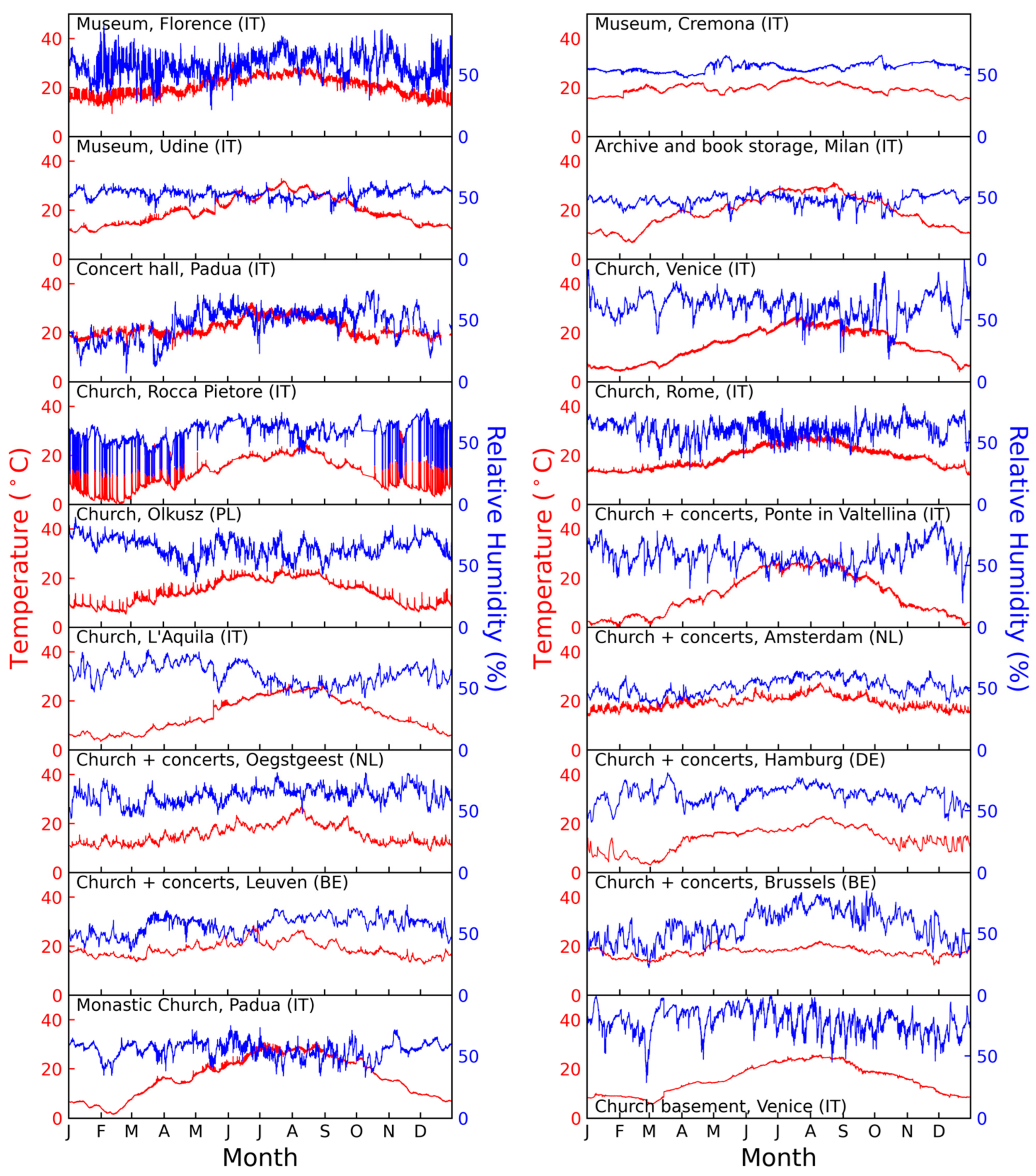
2.1. Datasets
2.2. Methods
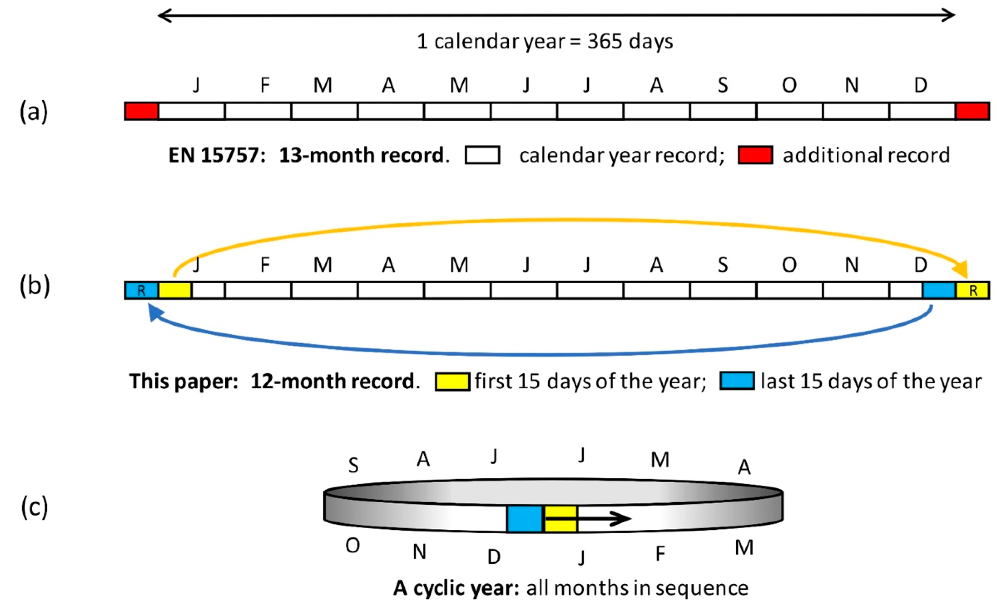
2.2.1. Datasets Necessary for the Determination of the Safe Band: 12 or 13 Months?
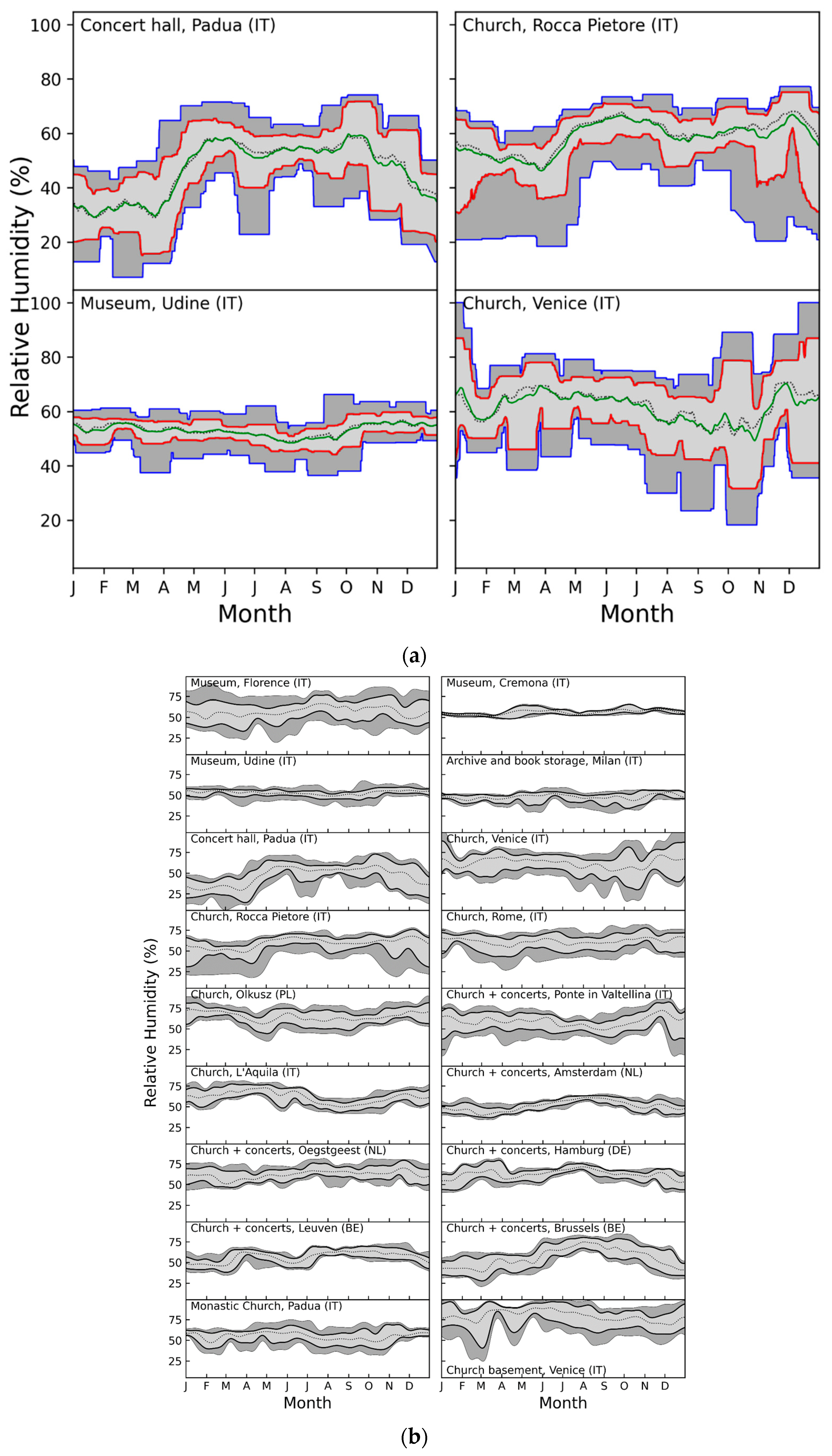
2.2.2. Method of the Informative Annex A: Fluctuations from the Centred Moving Average
2.2.3. Alternative Method: Interpolation of the Percentile Distribution
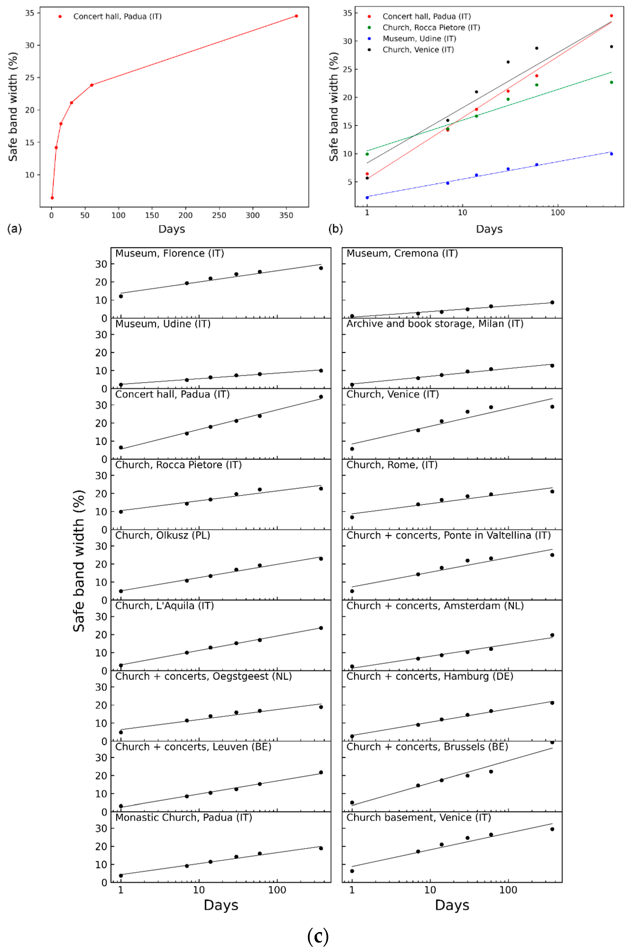
2.2.4. Evaluation of the Most Convenient Time Window
3. Results and Discussions
3.1. Comparison between the Two Methods: Centred Moving Average and Percentile Interpolation
3.2. Comparison between Different Time Windows
4. Language and Communication
5. Conclusions
Author Contributions
Funding
Institutional Review Board Statement
Informed Consent Statement
Data Availability Statement
Acknowledgments
Conflicts of Interest
References
- EN 15757 Standard; Conservation of Cultural Heritage—Specifications for Temperature and Relative Humidity to Limit Climate-Induced Mechanical Damage. European Committee for Standardization (CEN): Brussels, Belgium, 2010.
- Camuffo, D. Microclimate for Cultural Heritage—Measurement, Risk Assessment, Conservation, Restoration and Maintenance of Indoor and Outdoor Monuments, 3rd ed.; Elsevier: Amsterdam, The Netherlands, 2019. [Google Scholar]
- Camuffo, D. The European Standards on Environment and Cultural Heritage, and the Activity of WG4 Working Group at UNI. In La Normativa Tecnica Italiana Ed Europea Per Il Patrimonio Culturale. Atlanti Della Conservazione Del Patrimonio Culturale; Fassina, V., Ed.; Nardini: Florence, Italy, 2022; pp. 61–75. [Google Scholar]
- ASHRAE. Museums, Galleries, Archives and Libraries. In ASHRAE Handbook—HVAC Applications; American Society of Heating, Refrigerating, and Air-Conditioning Engineers: Atlanta, GA, USA, 2007; Chapter 21; pp. 21.1–21.23. [Google Scholar]
- ASHRAE. Museums, Galleries, Archives and Libraries. In ASHRAE Handbook—HVAC Applications; American Society of Heating, Refrigerating, and Air-Conditioning Engineers: Atlanta, GA, USA, 2011; Chapter 23; pp. 23.1–23.23. [Google Scholar]
- Michalski, S. The Ideal Climate, Risk Management, the ASHRAE Chapter, Proofed Fluctuations, and Toward a Full Risk Analysis Model. In Proceedings of the Contribution to the Experts’ Roundtable on Sustainable Climate Management Strategies, Tenerife, Spain, 23–27 April 2007; The Paul Getty Institute: Los Angeles, CA, USA, 2009. [Google Scholar]
- Bratasz, Ł.; Kozłowski, R.; Camuffo, D.; Pagan, E. Impact of Indoor Heating on Painted Wood. Monitoring the Altarpiece in the Church of Santa Maria Maddalena in Rocca Pietore, Italy. Stud. Conserv. 2007, 52, 199–210. [Google Scholar] [CrossRef]
- Camuffo, D.; Pagan, E.; Schellen, H.; Limpens-Neilen, D.; Kozlowski, R.; Bratasz, L.; Rissanen, S.; Van Grieken, R.; Spolnik, Z.; Bencs, L.; et al. Church Heating and Preservation of the Cultural Heritage: A Practical Guide to the Pros and Cons of Various Heating Systems; Electa Mondadori: Milano, Italy, 2007. [Google Scholar]
- Camuffo, D.; Pagan, E.; Rissanen, S.; Bratasz, Ł.; Kozłowski, R.; Camuffo, M.; della Valle, A. An Advanced Church Heating System Favourable to Artworks: A Contribution to European Standardisation. J. Cult. Herit. 2010, 11, 205–219. [Google Scholar] [CrossRef]
- Bratasz, Ł. Acceptable and Non-Acceptable Microclimate Variability: The Case of Wood. In Basic Environmental Mechanisms Affecting Cultural Heritage—Understanding Deterioration Mechanisms for Conservation Purposes; Camuffo, D., Fassina, V., Havermans, J., Eds.; COST Action D42 “Enviart”; Nardini: Florence, Italy, 2010; Chapter 4; pp. 49–58. [Google Scholar]
- Jakieła, S.; Bratasz, Ł.; Kozłowski, R. Acoustic Emission for Tracing the Evolution of Damage in Wooden Objects. Stud. Conserv. 2007, 52, 101–109. [Google Scholar] [CrossRef]
- Lukomski, M.; Strojecki, M.; Pretzel, B.; Blades, N.; Beltran, V.L.; Freeman, A. Acoustic Emission Monitoring of Micro-Damage in Wooden Art Objects to Assess Climate Management Strategies. Insight-Non-Destr. Test. Cond. Monit. 2017, 59, 256–264. [Google Scholar] [CrossRef]
- Califano, A.; Baiesi, M.; Bertolin, C. Analysing the Main Standards for Climate-Induced Mechanical Risk in Heritage Wooden Structures: The Case of the Ringebu and Heddal Stave Churches (Norway). Atmosphere 2022, 13, 791. [Google Scholar] [CrossRef]
- WMO. Guidelines on the Definition and Monitoring of Extreme Weather and Climate Events—TT-DEWCE WMO 14 April 2016; World Meteorological Organization: Geneva, Switzerland, 2016. [Google Scholar]
- IPCC. Climate Change 2014: Synthesis Report; Mach, K.J., Meyer, L.A., Pachauri, R.K., Planton, S., von Stechow, C., Eds.; Annex II: Glossary. Contribution of Working Groups I, II and III to the Fifth Assessment Report of the Intergovernmental Panel on Climate Change; IPCC: Geneva, Switzerland, 2014. [Google Scholar]
- Camuffo, D.; Bertolin, C.; Bonazzi, A.; Campana, F.; Merlo, C. Past, Present and Future Effects of Climate Change on a Wooden Inlay Bookcase Cabinet: A New Methodology Inspired by the Novel European Standard EN 15757:2010. J. Cult. Herit. 2014, 15, 26–35. [Google Scholar] [CrossRef]
- Bertolin, C.; Camuffo, D.; Bighignoli, I. Past Reconstruction and Future Forecast of Domains of Indoor Relative Humidity Fluctuations Calculated According to EN 15757:2010. Energy Build. 2015, 102, 197–206. [Google Scholar] [CrossRef]
- Taylor, T. Preservation of Cultural Heritage: The Design of Low-Energy Archival Storage. In Advanced Technologies for Sustainable Systems. Lecture Notes in Networks and Systems; Bahei-El-Din, Y., Hassan, M., Eds.; Springer: Berlin, Germany, 2017; Volume 4. [Google Scholar]
- Frasca, F.; Siani, A.M.; Casale, G.R.; Pedone, M.; Bratasz, L.; Strojecki, M.; Mleczkowska, A. Assessment of Indoor Climate of Mogiła Abbey in Kraków (Poland) and the Application of the Analogues Method to Predict Microclimate Indoor Conditions. Environ. Sci. Pollut. Res. 2017, 24, 13895–13907. [Google Scholar] [CrossRef]
- Leijonhufvud, G.; Broström, T. Standardizing the Indoor Climate in Historic Buildings: Opportunities, Challenges and Ways Forward. J. Archit. Conserv. 2018, 24, 3–18. [Google Scholar] [CrossRef] [Green Version]
- Żaba, A.; Marchacz, M. Historical Climate of the Historic Church of St. George at Ostropa. E3S Web Conf. 2018, 49, 00138. [Google Scholar] [CrossRef] [Green Version]
- Díaz-Arellano, I.; Zarzo, M.; García-Diego, F.J.; Perles, A. A Methodology for the Multi-Point Characterization of Short-Term Temperature Fluctuations in Complex Microclimates Based on the European Standard EN 15757:2010: Application to the Archaeological Museum of L’Almoina (Valencia, Spain). Sensors 2021, 22, 7754. [Google Scholar] [CrossRef] [PubMed]
- Manfriani, C.; Gualdani, G.; Goli, G.; Carlson, B.; Certo, A.R.; Mazzanti, P.; Fioravanti, M. The Contribution of IoT to the Implementation of Preventive Conservation According to European Standards: The Case Study of the “Cannone” Violin and Its Historical Copy. Sustainability 2021, 13, 1900. [Google Scholar] [CrossRef]
- Verticchio, E.; Frasca, F.; Bertolin, C.; Siani, A.M. Climate-Induced Risk for the Preservation of Paper Collections: Comparative Study Among three Historic Libraries in Italy. Build. Environ. 2021, 206, 108394. [Google Scholar] [CrossRef]
- Fabbri, K. Historic Climate in Heritage Building and Standard 15757: Proposal for a Common Nomenclature. Climate 2022, 10, 4. [Google Scholar] [CrossRef]
- Verticchio, E.; Frasca, F.; Cavalieri, P.; Tedonio, L.; Fugaro, D.; Siani, A.M. Conservation Risks for Paper Collections Induced by the Microclimate in the Repository of the Alessandrina Library in Rome (Italy). Herit. Sci. 2022, 10, 80. [Google Scholar] [CrossRef] [PubMed]
- Burt, J.E.; Barber, G.M.; Rigby, D.L. Elementary Statistics for Geographers, 3rd ed.; Guilford Press: New York, NY, USA, 2009. [Google Scholar]
- WMO. Guidelines on the Calculation of Climate Normals—WMO No. 1203; World Meteorological Organization: Geneva, Switzerland, 2017. [Google Scholar]
- Wei, W.W.S. Time Series Analysis; Addison-Wesley: Redwood City, CA, USA, 1990. [Google Scholar]
- Poularikas, A.D. Windows. In The Handbook of Formulas and Tables for Signal Processing; Poularikas, A.D., Ed.; CRC Press LLC: Boca Raton, FL, USA, 1999; Chapter 7; pp. 131–148. [Google Scholar]
- Galton, F. The Geometric Mean in Vital and Social Statistics. Proc. R. Soc. Lond. 1879, 29, 365–367. [Google Scholar]
- Hart, P.E. Lognormal Distribution. In Econometrics; Eatwell, J., Milgate, M., Newman, P., Eds.; Palgrave Macmillan: London, UK, 1990. [Google Scholar]
- Papalexiou, S.M.; Koutsoyiannis, D.; Makropoulos, C. How Extreme is Extreme? An Assessment of Daily Rainfall Distribution Tails. Hydrol. Earth Syst. Sci. 2013, 17, 851–862. [Google Scholar] [CrossRef] [Green Version]
- Colombo, D.; Abreu, D.; Ramos Martins, M. Application of Markovian Models in Reliability and Availability Analysis: Advanced Topics. In Safety and Reliability Modeling and Its Applications; Phamand, H., Ram, M., Eds.; Elsevier: Dordrecht, The Netherlands, 2021; pp. 91–160. [Google Scholar]
- Coles, S.G. An Introduction to Statistical Modeling of Extreme Values; Springer: New York, NY, USA, 2001. [Google Scholar]


| No | Name | Location | Use | Climate Control | Period |
|---|---|---|---|---|---|
| 1 | Uffizi Gallery ° | Florence (IT) | Museum | HVAC during opening hours; continuous RH control | 1998 |
| 2 | Ala Ponzone ° | Cremona (IT) | Museum | HVAC, humidity control | 2011 |
| 3 | Museo Vescovile ° | Udine (IT) | Museum | passive climate control; filtered light and shutter control | 2015–2016 |
| 4 | Ca’ Granda ° | Milano (IT) | Archive & book storage with restricted access | passive climate control | 2011–2012 |
| 5 | Liviano ° | Padua (IT) | Monumental concert hall | continuous basic heating + occasional extra heating | 2002–2003 |
| 6 | S. Maria Gloriosa dei Frari ° | Venice (IT) | Church; tourist attraction | modest local heating | 2009–2010 |
| 7 | S. Maria Maddalena ° | Rocca Pietore (IT) | Church | occasional winter heating | 2002–2003 |
| 8 | S. Maria Maggiore ° | Rome (IT) | Church; tourist attraction | no HVAC | 1996–1997 |
| 9 | St Andrew the Apostle ° | Olkusz (PO) | Church | occasional winter heating | 2007–2008 |
| 10 | Madonna di Campagna * | Valtellina (IT) | Church with concerts | no HVAC | 2003–2004 |
| 11 | S. Maria Collemaggio * | L’Aquila (IT) | Church with concerts | no HVAC | 2003–2004 |
| 12 | Walloon Church (Waalse Kerk) * | Amsterdam (NL) | Church with concerts | continuous winter heating | 2003–2004 |
| 13 | St Willibrord (Groene Kerk) * | Oegstgeest (NL) | Church with concerts | continuous winter heating | 2003–2004 |
| 14 | St Jacob * | Hamburg (GE) | Church with concerts | occasional winter heating | 2003–2004 |
| 15 | St Michael * | Leuven (BE) | Church with concerts | continuous winter heating | 2004–2005 |
| 16 | Notre Dame du Sablon * | Brussels (BE) | Church with concerts | uneven winter heating | 2004–2005 |
| 17 | Old Choir Monastic Church ° | Padua (IT) | Church with restricted access | no HVAC; almost unperturbed indoor climate | 2011–2012 |
| 18 | Church basement ° | Venice (IT) | Basement with restricted access | no HVAC; unperturbed indoor climate | 2020 |
| Variable | Definition | Example |
|---|---|---|
| n | sequential number of the reading sampled in the calendar day j | n = 1 is the first reading of the day j, starting from midnight; n = 2 is the second reading and so on |
| j | sequential number of the calendar day (1≤ j ≤ 365) | j = 45 represents the 45th day of the year, i.e., 14 February |
| RH(n, j) | individual readings of the record RH(n, j) | the nth value of RH recorded in the day j of the calendar year |
| <RHmo(n, j)> | average of RH calculated with the centred moving average, using a monthly window | <RHmo(n, 45)> for j= 45 (i.e., 14 February). It represents the average RH around the reading n, from j − 15 = 30 (i.e., 30 January) to j + 15 = 60 (i.e., 1 March) |
| ∆RH(n, j) | fluctuations defined as the difference RH(n, j) − <RHmo(n, j)> | difference between every individual reading RH(n, j) and the moving average <RHmo(n, j)> centred on it |
| <RHyr> | yearly average of RH | average from 1 January to 31 December |
| No | Case Study | a | b | 30-d Intercept |
|---|---|---|---|---|
| 1 | Museum, Florence (IT) | 2.70 | 13.76 | 22.9 |
| 2 | Museum, Cremona (IT) | 1.36 | 0.48 | 5.1 |
| 3 | Museum, Udine (IT) | 1.35 | 2.38 | 7.0 |
| 4 | Archive and book storage, Milan (IT) | 1.86 | 2.53 | 8.9 |
| 5 | Concert hall, Padua (IT) | 4.72 | 5.52 | 21.6 |
| 6 | Church, Venice (IT) | 4.26 | 8.34 | 22.8 |
| 7 | Church, Rocca Pietore (IT) | 2.37 | 10.49 | 18.6 |
| 8 | Church, Rome, (IT) | 2.44 | 8.72 | 17.0 |
| 9 | Church, Olkusz (PL) | 3.18 | 5.12 | 15.9 |
| 10 | Church + concerts, Ponte in Valtellina (IT) | 3.52 | 7.31 | 19.3 |
| 11 | Church, L’Aquila (IT) | 3.47 | 3.16 | 15.0 |
| 12 | Church + concerts, Amsterdam (NL) | 2.87 | 1.33 | 11.1 |
| 13 | Church + concerts, Oegstgeest (NL) | 2.41 | 6.36 | 14.6 |
| 14 | Church + concerts, Hamburg (DE) | 3.19 | 3.12 | 14.0 |
| 15 | Church + concerts, Leuven (BE) | 3.14 | 2.49 | 13.2 |
| 16 | Church + concerts, Brussels (BE) | 5.37 | 3.47 | 21.7 |
| 17 | Monastic Church, Padua (IT) | 2.65 | 4.27 | 13.3 |
| 18 | Church basement, Venice (IT) | 4.02 | 8.76 | 22.4 |
Publisher’s Note: MDPI stays neutral with regard to jurisdictional claims in published maps and institutional affiliations. |
© 2022 by the authors. Licensee MDPI, Basel, Switzerland. This article is an open access article distributed under the terms and conditions of the Creative Commons Attribution (CC BY) license (https://creativecommons.org/licenses/by/4.0/).
Share and Cite
Camuffo, D.; Della Valle, A.; Becherini, F. The European Standard EN 15757 Concerning Specifications for Relative Humidity: Suggested Improvements for Its Revision. Atmosphere 2022, 13, 1344. https://doi.org/10.3390/atmos13091344
Camuffo D, Della Valle A, Becherini F. The European Standard EN 15757 Concerning Specifications for Relative Humidity: Suggested Improvements for Its Revision. Atmosphere. 2022; 13(9):1344. https://doi.org/10.3390/atmos13091344
Chicago/Turabian StyleCamuffo, Dario, Antonio Della Valle, and Francesca Becherini. 2022. "The European Standard EN 15757 Concerning Specifications for Relative Humidity: Suggested Improvements for Its Revision" Atmosphere 13, no. 9: 1344. https://doi.org/10.3390/atmos13091344
APA StyleCamuffo, D., Della Valle, A., & Becherini, F. (2022). The European Standard EN 15757 Concerning Specifications for Relative Humidity: Suggested Improvements for Its Revision. Atmosphere, 13(9), 1344. https://doi.org/10.3390/atmos13091344