
Impacts of the Interannual Variability of the Kuroshio Extension on the East Asian Trough in Winter


Abstract
:1. Introduction
2. Data and Methodology
2.1. Data
2.2. Methodology
2.3. Estimating the Atmospheric Responses
3. Results
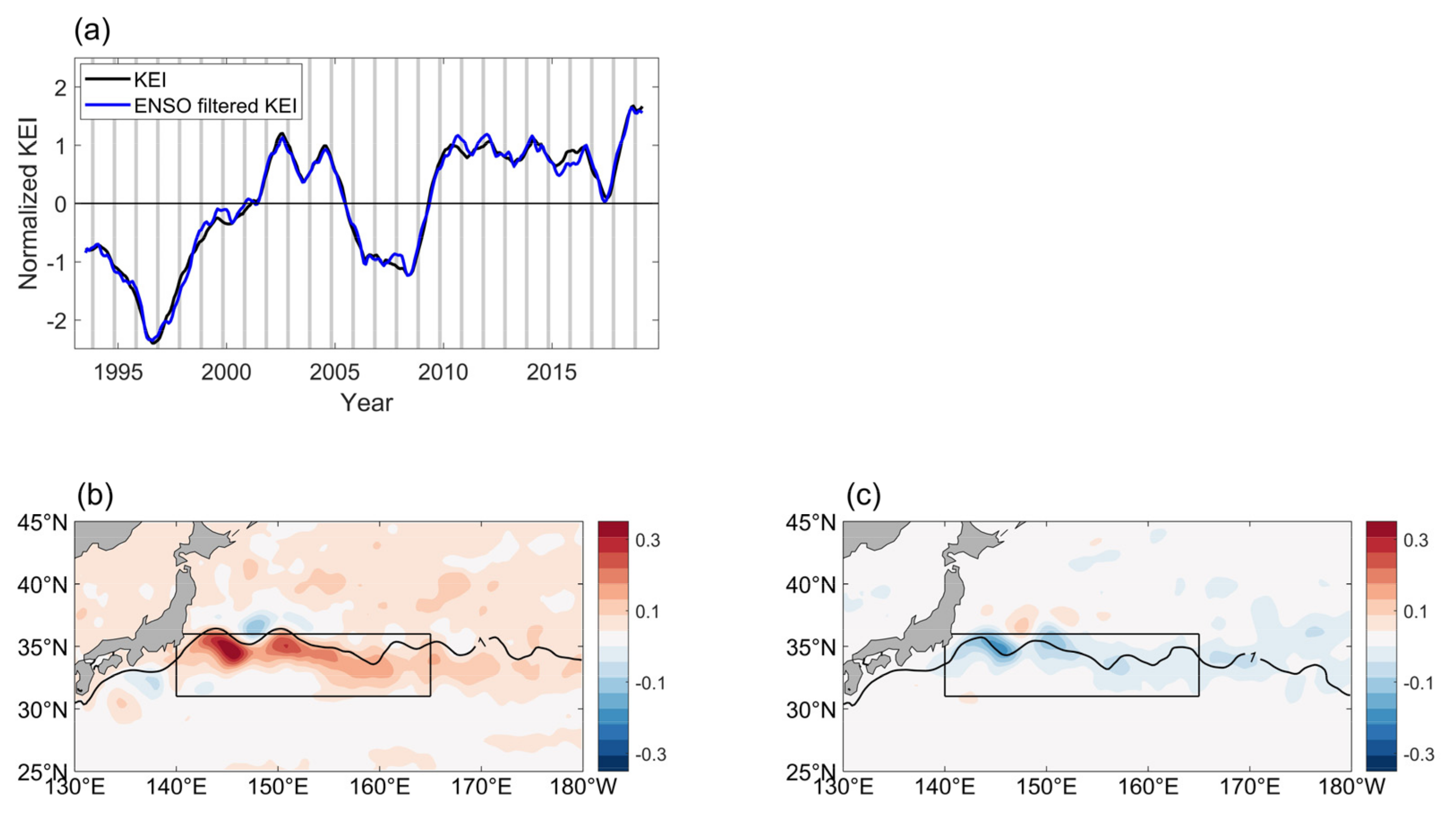
3.1. The KE Index
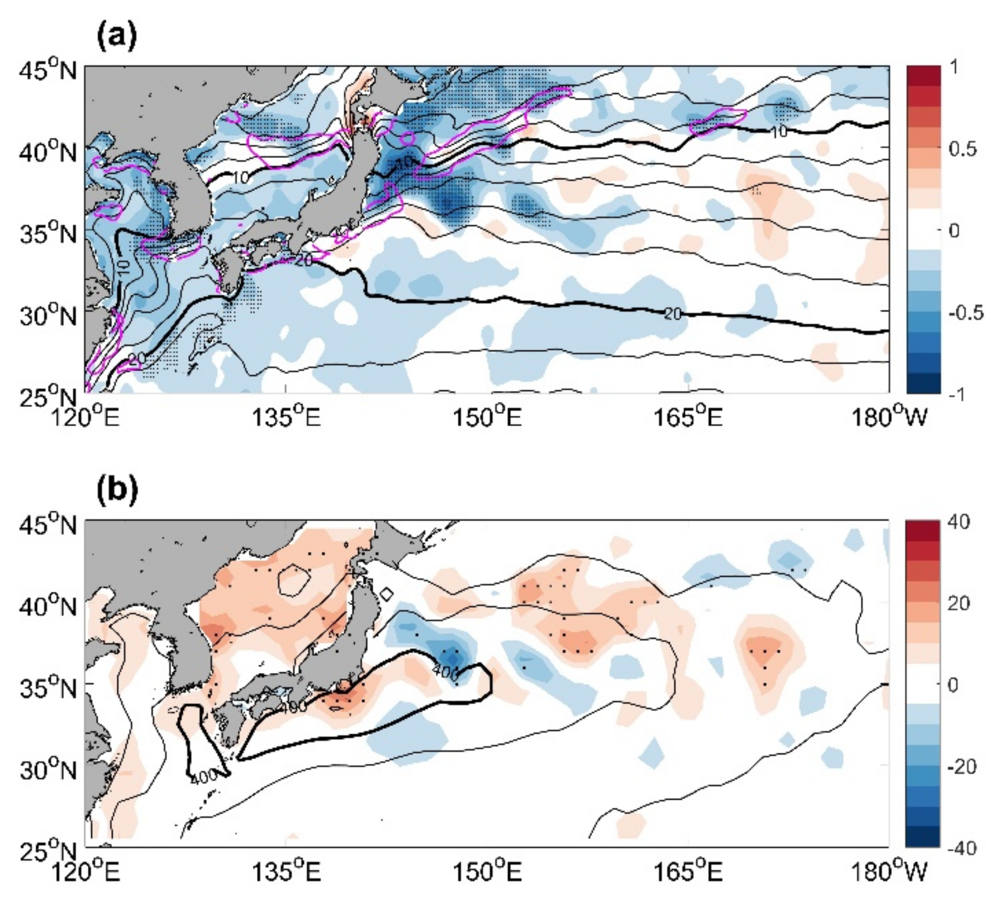
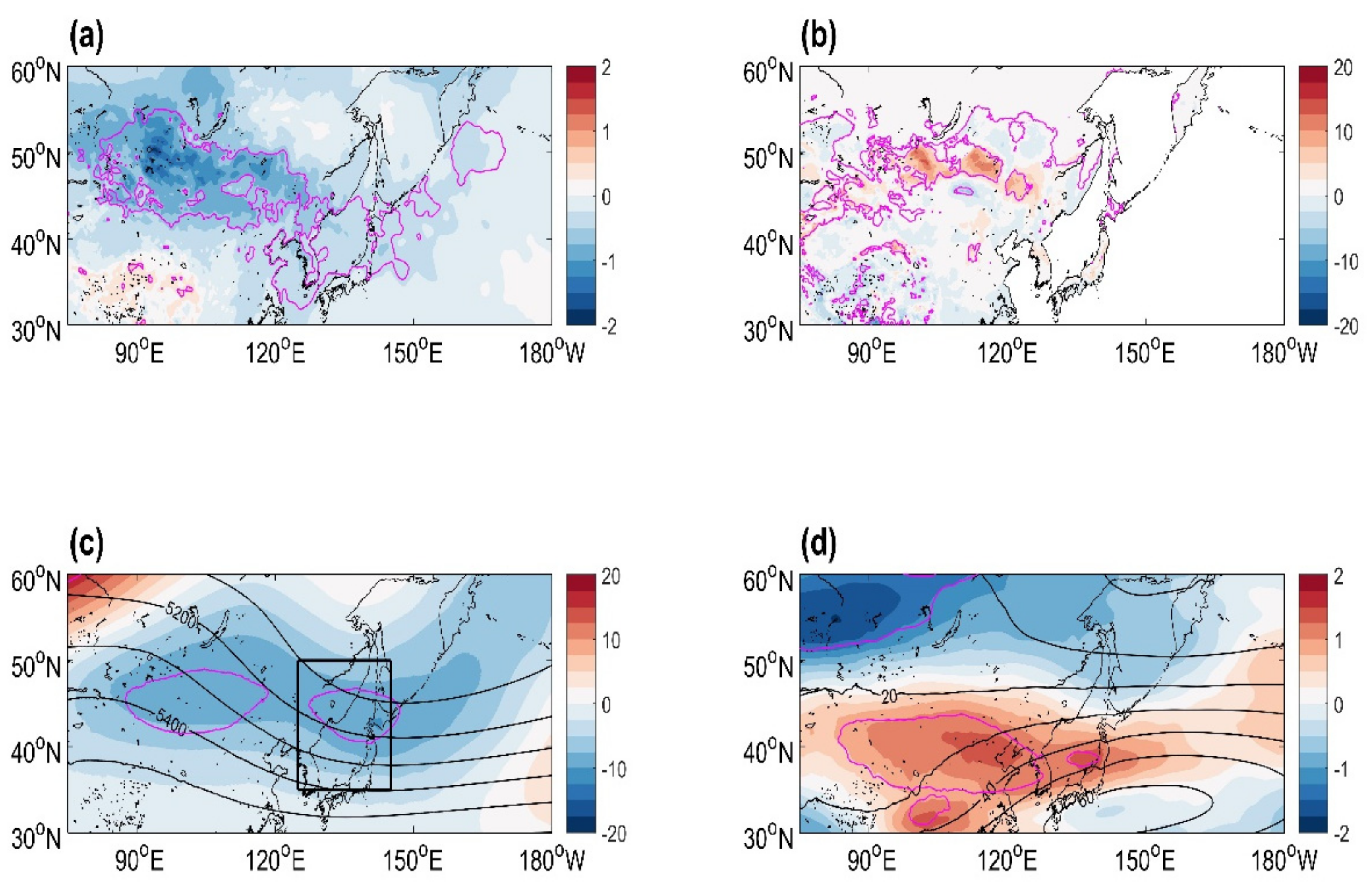
3.2. EAT Responses to the KE Variability
3.3. Possible Mechanisms
3.3.1. Rossby Wave Activity
3.3.2. Eddy–Mean Flow Interaction
3.3.3. Thermal Winds
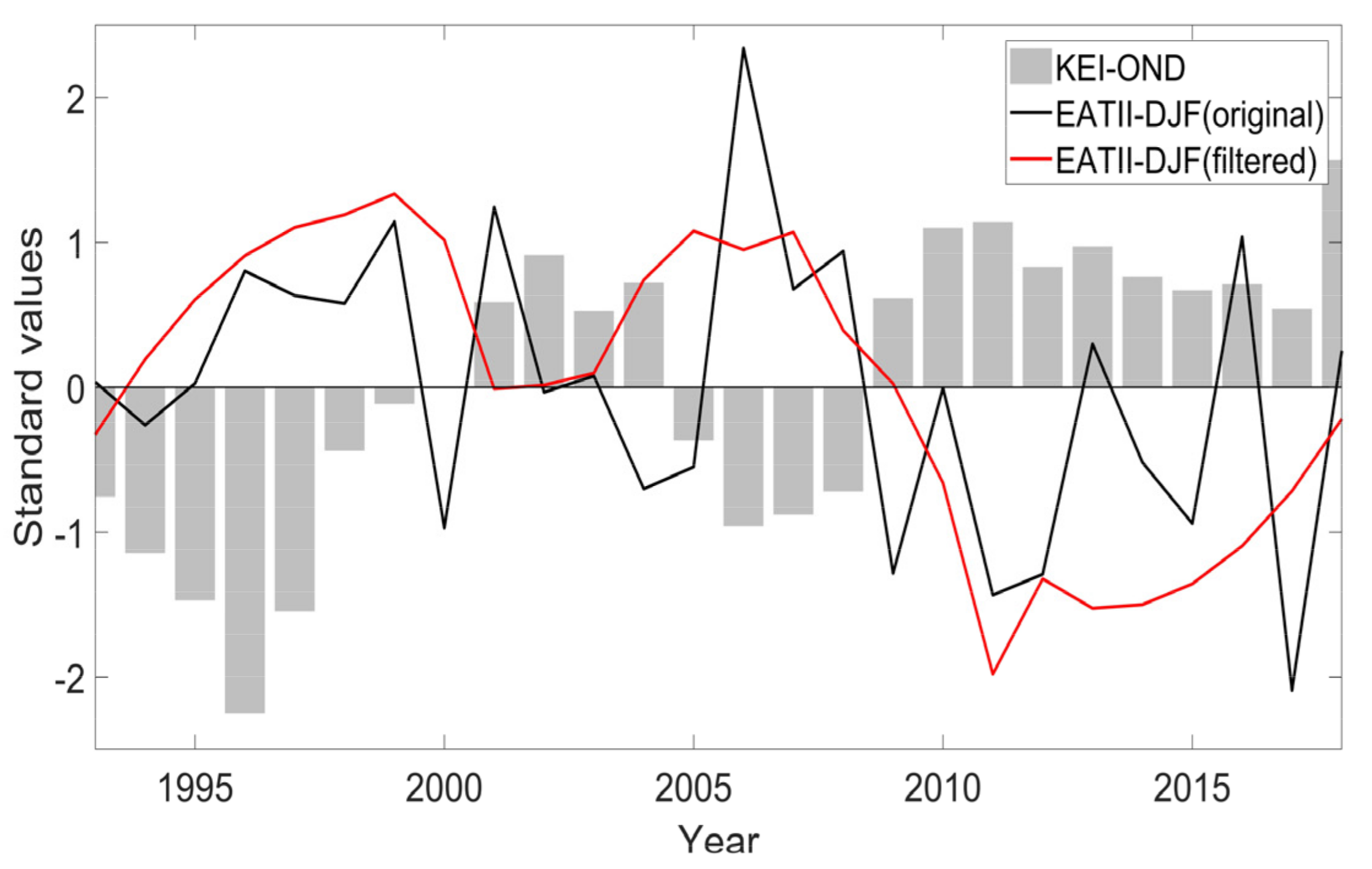
3.4. The Effects of KE Fluctuation on the East Asian Winter Climate
4. Conclusions and Discussion
Author Contributions
Funding
Institutional Review Board Statement
Informed Consent Statement
Data Availability Statement
Conflicts of Interest
References
- Wang, L.; Chen, W.; Zhou, W.; Huang, R. Interannual variations of East Asian trough axis at 500 hPa and its association with the East Asian winter monsoon pathway. J. Clim. 2009, 22, 600–614. [Google Scholar] [CrossRef] [Green Version]
- Zhang, Y.; Sperber, K.R.; Boyle, J.S. Climatology and interannual variation of the East Asian winter monsoon: Results from the 1979–95 NCEP/NCAR reanalysis. Mon. Weather Rev. 1997, 125, 2605–2619. [Google Scholar] [CrossRef]
- Nakamura, H.; Miyasaka, T.; Kosaka, Y.; Takaya, K.; Honda, M. Northern Hemisphere extratropical tropospheric planetary waves and their low-frequency variability: Their vertical structure and interaction with transient eddies and surface thermal contrasts. In Climate Dynamics: Why Does Climate Vary? John Wiley & Sons, Inc.: Hoboken, NJ, USA, 2010; Volume 189, pp. 149–179. [Google Scholar] [CrossRef]
- Smagorinsky, J. The dynamical influence of large-scale heat sources and sinks on the quasi-stationary mean motions of the atmosphere. Q. J. R. Meteorol. Soc. 1953, 79, 2–366. [Google Scholar] [CrossRef]
- Nakamura, H.; Izumi, T.; Sampe, T. Interannual and decadal modulations recently observed in the Pacific storm track activity and East Asian winter monsoon. J. Clim. 2002, 15, 1855–1874. [Google Scholar] [CrossRef]
- Ren, X.; Zhang, Y.; Xiang, Y. Connections between wintertime jet stream variability, oceanic surface heating, and transient eddy activity in the North Pacific. J. Geophys. Res. Atmos. 2008, 113, D21. [Google Scholar] [CrossRef] [Green Version]
- Ren, X.; Yang, X.; Chu, C. Seasonal variations of the synoptic-scale transient eddy activity and polar front jet over East Asia. J. Clim. 2010, 23, 3222–3233. [Google Scholar] [CrossRef]
- Wen, M.; Yang, S.; Kumar, A.; Zhang, P. An analysis of the large-scale climate anomalies associated with the snowstorms affecting China in January 2008. Mon. Weather Rev. 2009, 137, 1111–1131. [Google Scholar] [CrossRef]
- Zhou, W.; Chan, J.C.; Chen, W.; Ling, J.; Pinto, J.G.; Shao, Y. Synoptic-scale controls of persistent low Zuotemperature and icy weather over southern China in January 2008. Mon. Weather Rev. 2009, 137, 3978–3991. [Google Scholar] [CrossRef] [Green Version]
- Staff Members of the Section of Synoptic and Dynamic Meteorology, Institute of Geophysics and Meteorology, Academia Sinica, Peking. On the general circulation over Eastern Asia (II). Tellus 1958, 10, 58–75. [Google Scholar]
- Song, L.; Wang, L.; Chen, W.; Zhang, Y. Intraseasonal variation of the strength of the East Asian trough and its climatic impacts in boreal winter. J. Clim. 2016, 29, 2557–2577. [Google Scholar] [CrossRef]
- Gong, D.; Wang, S.; Zhu, J. East Asian winter monsoon and Arctic oscillation. Geophys. Res. Lett. 2001, 28, 2073–2076. [Google Scholar] [CrossRef]
- Feng, G.; Zou, M.; Qiao, S.; Zhi, R.; Gong, Z. The changing relationship between the December North Atlantic Oscillation and the following February East Asian trough before and after the late 1980s. Clim. Dyn. 2018, 51, 4229–4242. [Google Scholar] [CrossRef]
- Qiao, S.; Feng, G. Impact of the December North Atlantic oscillation on the following February East Asian trough. J. Geophys. Res. Atmos. 2016, 121, 10074–10088. [Google Scholar] [CrossRef] [Green Version]
- Luo, X.; Wang, B. How autumn Eurasian snow anomalies affect east Asian winter monsoon: A numerical study. Clim. Dyn. 2019, 52, 69–82. [Google Scholar] [CrossRef]
- Sun, C.; Yang, S.; Li, W.; Zhang, R.; Wu, R. Interannual variations of the dominant modes of East Asian winter monsoon and possible links to Arctic sea ice. Clim. Dyn. 2016, 47, 481–496. [Google Scholar] [CrossRef]
- Sun, J.; Wu, S.; Ao, J. Role of the North Pacific sea surface temperature in the East Asian winter monsoon decadal variability. Clim. Dyn. 2016, 46, 3793–3805. [Google Scholar] [CrossRef] [Green Version]
- Hao, X.; He, S.; Wang, H.; Han, T. Quantifying the contribution of anthropogenic influence to the East Asian winter monsoon in 1960–2012. Atmos. Chem. Phys. 2019, 19, 9903–9911. [Google Scholar] [CrossRef] [Green Version]
- Miao, J.; Wang, T.; Wang, H.; Zhu, Y.; Sun, J. Interdecadal weakening of the East Asian winter monsoon in the mid-1980s: The roles of external forcings. J. Clim. 2018, 31, 8985–9000. [Google Scholar] [CrossRef]
- Kelly, K.A.; Small, R.J.; Samelson, R.M.; Qiu, B.; Joyce, T.M.; Kwon, Y.O.; Cronin, M.F. Western boundary currents and frontal air–sea interaction: Gulf Stream and Kuroshio Extension. J. Clim. 2010, 23, 5644–5667. [Google Scholar] [CrossRef]
- Kwon, Y.O.; Alexander, M.A.; Bond, N.A.; Frankignoul, C.; Nakamura, H.; Qiu, B.; Thompson, L.A. Role of the Gulf Stream and Kuroshio–Oyashio systems in large-scale atmosphere–ocean interaction: A review. J. Clim. 2010, 23, 3249–3281. [Google Scholar] [CrossRef]
- Nonaka, M.; Xie, S.-P. Covariations of sea surface temperature and wind over the Kuroshio and its extension: Evidence for ocean-to-atmosphere feedback. J. Clim. 2003, 16, 1404–1413. [Google Scholar] [CrossRef]
- Small, R.D.; deSzoeke, S.P.; Xie, S.-P.; O’neill, L.; Seo, H.; Song, Q.; Cornillon, P.; Spall, M.; Minobe, S. Air–sea interaction over ocean fronts and eddies. Dyn. Atmos. Ocean. 2008, 45, 274–319. [Google Scholar] [CrossRef]
- Qiu, B.; Chen, S. Variability of the Kuroshio Extension jet, recirculation gyre, and mesoscale eddies on decadal time scales. J. Phys. Oceanogr. 2005, 35, 2090–2103. [Google Scholar] [CrossRef]
- Jiang, Y.; Zhang, S.; Xie, S.-P.; Chen, Y.; Liu, H. Effects of a Cold Ocean Eddy on Local Atmospheric Boundary Layer Near the Kuroshio Extension: In Situ Observations and Model Experiments. J. Geophys. Res. Atmos. 2019, 124, 5779–5790. [Google Scholar] [CrossRef]
- Ma, J.; Xu, H.; Dong, C.; Lin, P.; Liu, Y. Atmospheric responses to oceanic eddies in the Kuroshio Extension region. J. Geophys. Res. Atmos. 2015, 120, 6313–6330. [Google Scholar] [CrossRef]
- Wang, Y.; Liu, W. Observational evidence of frontal-scale atmospheric responses to Kuroshio Extension variability. J. Clim. 2015, 28, 9459–9472. [Google Scholar] [CrossRef]
- Wang, Q.; Zhang, S.; Xie, S.-P.; Norris, J.R.; Sun, J.; Jiang, Y. Observed Variations of the Atmospheric Boundary Layer and Stratocumulus over a Warm Eddy in the Kuroshio Extension. Mon. Weather Rev. 2019, 147, 1581–1591. [Google Scholar] [CrossRef]
- Ma, X.; Chang, P.; Saravanan, R.; Montuoro, R.; Hsieh, J.S.; Wu, D.; Lin, X.; Wu, L. Distant influence of Kuroshio eddies on North Pacific weather patterns? Sci. Rep. 2015, 5, 17785. [Google Scholar] [CrossRef] [Green Version]
- Ma, X.; Chang, P.; Saravanan, R.; Montuoro, R.; Nakamura, H.; Wu, D.; Lin, X.; Wu, L. Importance of resolving Kuroshio front and eddy influence in simulating the North Pacific storm track. J. Clim. 2017, 30, 1861–1880. [Google Scholar] [CrossRef]
- O’Reilly, C.H.; Czaja, A. The response of the Pacific storm track and atmospheric circulation to Kuroshio Extension variability. Q. J. R. Meteorol. Soc. 2015, 141, 52–66. [Google Scholar] [CrossRef]
- Révelard, A.; Frankignoul, C.; Sennéchael, N.; Kwon, Y.O.; Qiu, B. Influence of the decadal variability of the Kuroshio Extension on the atmospheric circulation in the cold season. J. Clim. 2016, 29, 2123–2144. [Google Scholar] [CrossRef]
- Taguchi, B.; Nakamura, H.; Nonaka, M.; Komori, N.; Kuwano-Yoshida, A.; Takaya, K.; Goto, A. Seasonal Evolutions of Atmospheric Response to Decadal SST Anomalies in the North Pacific Subarctic Frontal Zone: Observations and a Coupled Model Simulation. J. Clim. 2012, 25, 111–139. [Google Scholar] [CrossRef]
- Révelard, A.; Frankignoul, C.; Kwon, Y.O. A multivariate estimate of the cold season atmospheric response to North Pacific SST variability. J. Clim. 2018, 31, 2771–2796. [Google Scholar] [CrossRef]
- Ducet, N.; Le Traon, P.Y.; Reverdin, G. Global high-resolution mapping of ocean circulation from TOPEX/Poseidon and ERS-1 and -2. J. Geophys. Res. Ocean. 2000, 105, 19477–19498. [Google Scholar] [CrossRef]
- Yu, L.; Weller, R.A. Objectively analyzed air–sea heat fluxes for the global ice-free oceans (1981–2005). Bull. Am. Meteorol. Soc. 2007, 88, 527–540. [Google Scholar] [CrossRef] [Green Version]
- Qiu, B.; Chen, S.; Schneider, N.; Taguchi, B. A coupled decadal prediction of the dynamic state of the Kuroshio Extension system. J. Clim. 2014, 27, 1751–1764. [Google Scholar] [CrossRef] [Green Version]
- Sardeshmukh, P.D.; Hoskins, B.J. The generation of global rotational flow by steady idealized tropical divergence. J. Atmos. Sci. 1988, 45, 1228–1251. [Google Scholar] [CrossRef] [Green Version]
- Takaya, K.; Nakamura, H. A formulation of a wave-activity flux for stationary Rossby waves on a zonally varying basic flow. Geophys. Res. Lett. 1997, 24, 2985–2988. [Google Scholar] [CrossRef]
- Takaya, K.; Nakamura, H. A formulation of a phase-independent wave-activity flux for stationary and migratory quasigeostrophic eddies on a zonally varying basic flow. J. Atmos. Sci. 2001, 58, 608–627. [Google Scholar] [CrossRef]
- Hoskins, B.J.; Valdes, P.J. On the existence of storm-tracks. J. Atmos. Sci. 1990, 47, 1854–1864. [Google Scholar] [CrossRef]
- Sun, Z.; Zhang, J. Statistical characteristics of 40–60 day oscillation in extratropical area. In Proceedings of the Long-Term Weather Forecast; Ocean Press: Beijing, China, 1992; pp. 29–35. [Google Scholar]
- Lau, N.C.; Nath, M.J. Model simulation and projection of European heat waves in present-day and future climates. J. Clim. 2014, 27, 3713–3730. [Google Scholar] [CrossRef]
- Bretherton, C.S.; Widmann, M.; Dymnikov, V.P.; Wallace, J.M.; Bladé, I. The Effective Number of Spatial Degrees of Freedom of a Time-Varying Field. J. Clim. 1999, 12, 1990–2009. [Google Scholar] [CrossRef]
- Ferreira, D.; Frankignoul, C. The transient atmospheric response to midlatitude SST anomalies. J. Clim. 2005, 18, 1049–1067. [Google Scholar] [CrossRef]
- Ferreira, D.; Frankignoul, C. Transient atmospheric response to interactive SST anomalies. J. Clim. 2008, 21, 576–583. [Google Scholar] [CrossRef]
- Frankignoul, C.; Czaja, A.; L’Heveder, B. Air–sea feedback in the North Atlantic and surface boundary conditions for ocean models. J. Clim. 1998, 11, 2310–2324. [Google Scholar] [CrossRef] [Green Version]
- Liu, Z.; Wu, L. Atmospheric Response to North Pacific SST: The Role of Ocean–Atmosphere Coupling. J. Clim. 2004, 17, 1859–1882. [Google Scholar] [CrossRef] [Green Version]
- Liu, Z.; Wen, N.; Liu, Y. On the assessment of nonlocal climate feedback. Part I: The generalized equilibrium feedback assessment. J. Clim. 2008, 21, 134–148. [Google Scholar] [CrossRef] [Green Version]
- Frankignoul, C.; Sennéchael, N.; Kwon, Y.O.; Alexander, M.A. Influence of the meridional shifts of the Kuroshio and the Oyashio Extensions on the atmospheric circulation. J. Clim. 2011, 24, 762–777. [Google Scholar] [CrossRef]
- Lei, T.; Li, S.; Luo, F.; Liu, N. Two dominant factors governing the decadal cooling anomalies in winter in East China during the global hiatus period. Int. J. Climatol. 2020, 40, 750–768. [Google Scholar] [CrossRef]
- Zhang, M.; Perrie, W.; Long, Z. Springtime North Pacific Oscillation and summer sea ice in the Beaufort sea. Clim. Dyn. 2019, 53, 671–686. [Google Scholar] [CrossRef]
- Chang, E.K. Are the Northern Hemisphere winter storm tracks significantly correlated? J. Clim. 2004, 17, 4230–4244. [Google Scholar] [CrossRef]
- Drouard, M.; Rivière, G.; Arbogast, P. The North Atlantic Oscillation response to large-scale atmospheric anomalies in the northeastern Pacific. J. Atmos. Sci. 2013, 70, 2854–2874. [Google Scholar] [CrossRef]
- Song, L.; Wu, R. Comparison of intraseasonal East Asian winter cold temperature anomalies in positive and negative phases of the Arctic Oscillation. J. Geophys. Res. Atmos. 2018, 123, 8518–8537. [Google Scholar] [CrossRef]
- Zhou, B.; Xu, Y.; Shi, Y. Present and future connection of Asian-Pacific Oscillation to large-scale atmospheric circulations and East Asian rainfall: Results of CMIP5. Clim. Dyn. 2018, 50, 17–29. [Google Scholar] [CrossRef]
- Zuo, J.; Ren, H.; Xue, B.; Li, W. Predictability of winter temperature in China from previous autumn Arctic sea ice. Clim. Dyn. 2016, 47, 2331–2343. [Google Scholar] [CrossRef]
- Sakamoto, T.T.; Hasumi, H.; Ishii, M.; Emori, S.; Suzuki, T.; Nishimura, T.; Sumi, A. Responses of the Kuroshio and the Kuroshio Extension to global warming in a high-resolution climate model. Geophys. Res. Lett. 2005, 32. [Google Scholar] [CrossRef]
- Wu, L.; Cai, W.; Zhang, L.; Nakamura, H.; Timmermann, A.; Joyce, T.; McPhaden, M.J.; Alexander, M.; Qiu, B.; Visbeck, M.; et al. Enhanced warming over the global subtropical western boundary currents. Nat. Clim. Chang. 2012, 2, 161–166. [Google Scholar] [CrossRef]
- Zhang, X.; Wang, Q.; Mu, M. The impact of global warming on Kuroshio Extension and its southern recirculation using CMIP5 experiments with a high-resolution climate model MIROC4h. Theor. Appl. Climatol. 2017, 127, 815–827. [Google Scholar] [CrossRef]


| AO | NAO | APO | Eurasian Snow Cover | Arctic Sea Ice Area | North Pacific SST | Kuroshio SST | |
|---|---|---|---|---|---|---|---|
| KEI | 0.08 | 0.44 * | 0.05 | 0.28 | −0.12 | −0.03 | −0.18 |
| EATI | −0.14 | −0.07 | 0.14 | −0.19 | 0.16 | 0.23 | 0.28 |
Publisher’s Note: MDPI stays neutral with regard to jurisdictional claims in published maps and institutional affiliations. |
© 2022 by the authors. Licensee MDPI, Basel, Switzerland. This article is an open access article distributed under the terms and conditions of the Creative Commons Attribution (CC BY) license (https://creativecommons.org/licenses/by/4.0/).
Share and Cite
Sun, J.; Zhang, S.; Jiang, Y.; Wang, Y.; Wu, B.; Wang, H. Impacts of the Interannual Variability of the Kuroshio Extension on the East Asian Trough in Winter. Atmosphere 2022, 13, 996. https://doi.org/10.3390/atmos13070996
Sun J, Zhang S, Jiang Y, Wang Y, Wu B, Wang H. Impacts of the Interannual Variability of the Kuroshio Extension on the East Asian Trough in Winter. Atmosphere. 2022; 13(7):996. https://doi.org/10.3390/atmos13070996
Chicago/Turabian StyleSun, Jianxiang, Suping Zhang, Yuxi Jiang, Yanshuo Wang, Baoqin Wu, and Haijiao Wang. 2022. "Impacts of the Interannual Variability of the Kuroshio Extension on the East Asian Trough in Winter" Atmosphere 13, no. 7: 996. https://doi.org/10.3390/atmos13070996
APA StyleSun, J., Zhang, S., Jiang, Y., Wang, Y., Wu, B., & Wang, H. (2022). Impacts of the Interannual Variability of the Kuroshio Extension on the East Asian Trough in Winter. Atmosphere, 13(7), 996. https://doi.org/10.3390/atmos13070996