Abstract
Novaya Zemlya bora is a strong downslope windstorm in the east of the Barents Sea. This paper considers the influence of the Novaya Zemlya bora on the turbulent heat exchange between the atmosphere and the ocean and on processes in the ocean. Another goal of this study is to demonstrate the sensitivity of simulated turbulent fluxes during bora to model coupling between atmosphere, ocean and sea waves. In this regard, a high-resolution numerical simulation of one winter bora episode was carried out using the COAWST (Coupled-Ocean-Atmosphere-Wave-Sediment Transport) modeling system, which includes the atmospheric (WRF-ARW model), oceanic (ROMS model), and sea waves (SWAN model) components. As shown by the simulation results, in the fully coupled experiment, turbulent heat exchange is enhanced in comparison with the uncoupled experiment (by 3% on average over the region). This is due to the atmosphere-sea-waves interaction, and the results are highly sensitive to the choice of roughness parameterization. The influence of the interaction of the atmospheric and oceanic components on turbulent fluxes in this episode is small on average. Bora has a significant impact on the processes in the ocean directly near the coast, forming a strong coastal current and making a decisive contribution to the formation of dense waters. In the open sea, the bora, or rather, the redistribution of the wind and temperature fields caused by the orography of Novaya Zemlya, leads to a decrease in ocean heat content losses due to a decrease in turbulent heat exchange in comparison with the experiment with flat topography.
1. Introduction
A great number of studies using state-of-the-art earth system models, primarily regional climate models, demonstrate the need for atmosphere-ocean coupling on seasonal and climatic scales for different regions of the world [1]. Coupling primarily affects the sea surface temperature and heat fluxes and removes both positive and negative biases, which are present in the uncoupled models [2,3,4,5]. Air-sea coupling indirectly affects precipitation [6,7] and ocean characteristics (e.g., [8]), including ocean currents [3]. The main positive coupling effect is found in the tropics, especially in the Indian Ocean region when modeling the monsoon and associated precipitation (e.g., [7,9]), and also in the East Asian monsoon region [10]. Benefits of coupling have also been found in Europe (e.g., [11,12]) and for sea ice modeling in the Arctic [13,14].
In recent decades, coupled modeling has been used not only in climate studies, but also for lesser time scales. Many modern numerical weather prediction systems, for example, in Canada [15] and in the European Centre for Medium-Range Weather Forecasts [16], use coupled models of atmosphere and ocean and the effect of coupling on weather forecasts is significant [17]. For mesoscale phenomena, model coupling make sense if the mesoscale object is relatively long-lived (sufficient to affect the processes in the ocean) and is accompanied by strong interaction between the atmosphere and the ocean (for example, in strong winds). One of the most representative examples of such an object is the phenomenon of tropical cyclones, which are the subject of a large number of studies on coupled modeling (e.g., [18,19,20]). More recently, coupled modeling has been applied to polar lows [21]. Coupling is of great importance for modeling mesoscale phenomena in upwelling coastal regions (e.g., [22,23,24].
On the other hand, the effect of model coupling for both regional climate and weather events sometimes is not obvious [4,12,20,25,26]. The results of coupled modeling still could give biased values [7,27]. Therefore, the added value of the coupled simulations is still arguable (given the relative high cost of such simulations), and for each region and for each phenomenon sensitivity experiments are needed to reveal the impact of the model coupling.
Orographic winds, such as downslope windstorms, sometimes reach hurricane strength and are accompanied by sudden temperature changes. Therefore, under such conditions, a strong interaction of the atmosphere with the ocean should be expected. For example, significant differences in heat fluxes between coupled and uncoupled simulations was found for Adriatic bora [28,29]. Taking into account the interaction between the ocean and the atmosphere under bora conditions improves simulated turbulent heat fluxes [5]. In turn, increased ocean-atmosphere heat exchange during orographic winds affects the heat content of the upper ocean, its stratification, and can provoke deep convection in the ocean [30]. In addition, strong and frequent coastal winds affect the water circulation, sediment transport and biological characteristics in the coastal zone [6]. These anomalies can be carried by currents to other regions.
Warm Atlantic waters spread to the Barents Sea and enhance ocean-atmosphere heat exchange. This process is especially pronounced during cold-air outbreaks and strong winds. The Novaya Zemlya bora is the strongest and very frequent orographic wind in the Barents Sea [31,32]. According to the Malye Karmakuly weather station, the bora on the western coast of Novaya Zemlya (hereafter, “NZ”) is observed on average 138 days a year, with 25% of the wind speed exceeding 20 m s−1 [33]. The maximum measured wind gusts reach 50 m/s on the southern island and 60 m s−1 on the northern island. Bora is observed in all seasons (although it is rarely strong in the warm season) and can last up to 17 days.
Under the conditions of the Novaya Zemlya bora, the following processes, caused by air-sea interaction, are expected: (1) the formation of young and steep waves with high roughness; (2) strong mechanical mixing of the upper layer of the ocean due to strong wind and waves; (3) intense turbulent heat exchange between the ocean and the atmosphere and evaporation of moisture from the ocean surface due to high wind speed and low air temperature and humidity; (4) cooling and salinization of the upper layer of the ocean due to heat exchange with the atmosphere and increased evaporation and (5) the resulting intensification of convective mixing in the ocean, as well as (6) water densification; (7) modification of ocean currents. Some impact of air-sea interaction during bora on the Atlantic waters could be expected, since one of the branches of the warm current flows not too far from NZ. As for water densification, the western coast of NZ is a known region of dense water formation in polynyas during the cold season [34]. These polynyas are usually formed under the action of a strong wind from the shore, i.e., bora. The dense water formed in the polynyas is the source of the Arctic Intermediate and Bottom Water.
The following effects of model coupling are considered in this study. Firstly, the two-way coupling of atmospheric and sea waves models is expected to influence the sea surface roughness (most likely increasing it), and, consequently, turbulent exchange and wind speed. Secondly, the interaction between atmospheric and oceanic models should lead to a cooling of the sea surface temperature and, consequently, to a decrease in turbulent heat transfer. The effect of coupling between sea waves and ocean models is not so obvious for the phenomena under consideration, though it also could appear in the simulation results.
Since the effect of model coupling can be ambiguous, and its usefulness for Novaya Zemlya bora has never been explored before, one of the main goals of this study is to evaluate the effect of model coupling on simulated turbulent fluxes during the Novaya Zemlya bora. At the same time, we do not seek to determine which model—coupled or uncoupled—gives the best results compared to the observation, since the number of observations in this region is not sufficient for robust verification. Another goal is to evaluate the effect of the bora itself on air-sea heat exchange and on the processes in the ocean listed above. For this study, we chose an episode of strong bora, which was observed in December 2006. At this time of the year, the bora is already becoming strong and quite long, but the western coast of NZ is not yet completely ice-covered.
The main method of this study is a mixture of sensitivity tests and factor separation method. Several coupling strategies and parametrizations controlling the momentum transfer were tested. The effect of bora was distinguished by comparison of numerical experiments with and without NZ orography. One of the goals of identifying the bora effect is to show how important it is to take bora into account in turbulent flux estimates. Most flux estimates in the Barents Sea are made on the basis of reanalyses (e.g., [35,36]), which, due to their poor resolution, are not able to resolve the bora accurately.
The paper is organized as follows. Section 2 describes the design of numerical experiments and the models used. Section 3.1 is devoted to a general review of modeling results and their verification. The impact of model coupling on turbulent fluxes under bora conditions is considered in Section 3.2. The impact of bora itself on turbulent heat fluxes, as well as on ocean mixing, heat content and circulation is shown in Section 3.3. A discussion of the results and conclusions is given in Section 4.
2. Materials and Methods
2.1. COAWST Model
The study is based on simulation results obtained using the COAWST (Coupled-Ocean-Atmosphere-Wave-Sediment Transport) modeling system [37] version 3.6. This system links the models of the atmosphere (Weather Research and Forecasting model, hereafter “WRF”), the ocean (Regional Ocean Modeling System, ROMS) and sea waves (Simulating Waves Nearshore, SWAN) and using the Model Coupling Toolkit [38] models communicate with each other online. The ocean model receives from the atmospheric model the fluxes of heat, momentum and moisture, pressure and solar radiation (i.e., upper boundary conditions), and from the wave model the wave parameters to calculate wave-induced mixing. The atmospheric model receives SST from the ocean model, and significant wave height (SWH), average wavelength, and peak period to calculate the roughness length from the wave model. There are three options of roughness length calculation in a coupled mode: parametrizations of Taylor and Yelland [39] (hereafter—“Taylor_Yelland”), Oost et al. [40] (hereafter—“Oost”) and Drennan et al. [41] (hereafter—“Drennan”). In the “Taylor_Yelland” parameterization, the roughness length depends on the steepness of the waves, in “Oost” it depends on the reciprocal wave age and wavelength, in “Drennan” it depends on the reciprocal wave age and wave height. Finally, the wave model receives wind from the atmospheric model and currents and sea level data from the ocean model. For more details on the design of the model, see [37].
In recent versions of COAWST, there is no ability to simulate the sea ice. So, a sea ice parametrization of Budgell [42] from the Hedstrom’s version of ROMS model (https://github.com/kshedstrom/roms, accessed on 10 July 2022) was adapted for COAWST and added as a part of the ocean model. This sea ice model is based on ice thermodynamics from [43] and elastic-viscous-plastic rheology from [44,45]. It performs quite well in the Barents Sea, as shown by comparison with satellite observations of sea ice, especially in winter [42,46].
2.2. Atmospheric Model
The initial and boundary conditions for the atmospheric model WRF [47] were taken from the ERA5 reanalysis. Test runs with different initial data showed that the runs started from the ERA5 reanalysis outperformed those that started from ASR and CFSR reanalysis. Spectral nudging to reanalysis data above the boundary layer every 6 h prevented the simulated atmospheric circulation from deviating too much from the reanalysis. In experiments without interaction with the ocean model, the SST was taken from SODA (Simple Ocean Data Assimilation) ocean reanalysis (from which the ocean model starts) so that all experiments started from the same SST. Due to the coarse resolution of the land/sea mask in oceanic reanalysis, in some few grid nodes (mainly in the southeast of the region, in the Kara Sea), there was no information on SST; data from the ERA5 was used there. The initial sea ice field was a mixture of ice concentration and snow on ice from AMSR-E/Aqua data with 12.5-km resolution and ice thickness from ASR (Arctic System Reanalysis) v2. For simplicity, the same SST and sea ice were maintained throughout the calculation in experiments without coupling with the ocean model.
Preliminary simulations have shown that the wind speed and temperature during bora at Malye Karmakuly station are best reproduced using the Quasi–normal Scale Elimination (QNSE) [48] boundary layer parametrization, which is consistent with the previous results [49]. In the COAWST model, only Mellor–Yamada–Janjic and Mellor–Yamada Nakanishi Niino boundary layer schemes contain the parameterizations of sea surface roughness depending on the wave parameters. Therefore, these roughness parametrizations were added to the QNSE parameterization as well. It has previously been shown that changing land-use parameters to more realistic ones and reducing the tabular roughness coefficient for the tundra to more realistic values also significantly improves the results of modeling downslope windstorms in the Arctic [49]. Therefore, the land use and roughness parameter for the tundra on Novaya Zemlya was also changed here in accordance with the study of Shestakova [49]. The remaining parametrizations in the WRF model were as follows: the WRF Single-Moment 6-class parametrization of cloud microphysics [50], the Rapid Radiative Transfer Model for Global Climate Models parametrization of radiation fluxes [51], the Noah land surface parametrization [52]. The integration time step was set at 18 s.
2.3. Ocean Model
The ROMS model [53] was initialized from the SODA 3.3.2 reanalysis with 0.25° spatial resolution [54]. This reanalysis has been prepared using atmospheric forcing from the MERRA2 reanalysis. It has a time resolution of 5 days (averaged fields), and for the considered bora episode, the file with the central date of 7 December 2006, i.e., an average from 5 to 9 December, was chosen as an initial field. The initial sea ice concentration, ice thickness and snow thickness on ice for the ocean model were the same as for the atmospheric model; initial ice velocities were set to zero; sea ice temperature was set from ERA5 reanalysis. The tides were set from the OSU (Oregon State University) TPXO database, which is a product of a barotropic tide model with the assimilation of the TOPEX/Poseidon altimeter data [55]. Vertical mixing in ROMS was set using the Mellor–Yamada level 2.5 parameterization [56]. Bathymetry was set according to ETOPO2 database with 2′ spatial resolution. The open boundary conditions were taken from SODA (the same file as initial data) and set constant throughout the calculation. The following boundary-conditions options were used: the Chapman option [57] for surface elevation, the radiation and nudging scheme [58] for baroclinic velocity, the Flather option [59] for barotropic velocity, and the gradient scheme for scalars (including sea ice parameters). The baroclinic integration step was 15 s.
2.4. Sea Waves Model
The SWAN model ran in third-generation mode, taking into account wave breaking in the open sea and in shallow water and quadriplet interactions by default. Triadic wave interactions were not taken into account. Most of the experiments involving the wave model were carried out with the Komen formulation of wind-waves growth [60] (hereafter—“Komen”). The default bottom friction was used [61] with a constant of 0.067 m2 s−3. SWAN model started from the previously calculated wave spectra (so called “hot start”) to account for the effect of ocean swell from the North Atlantic. We ran the SWAN model coupled with the WRF model for four days prior to the start of the main experiments (i.e., from 5 to 8 December 2006) with two nested domains: the outer one, with a grid spacing of 15 km, covered most of the North Atlantic; the inner one, with a grid spacing of 3 km, coincided with the domain used for the main experiments (Figure 1). The GFS FNL analysis with a resolution of 1° was used as the boundary and initial conditions for the WRF model in these preparatory calculations.

Figure 1.
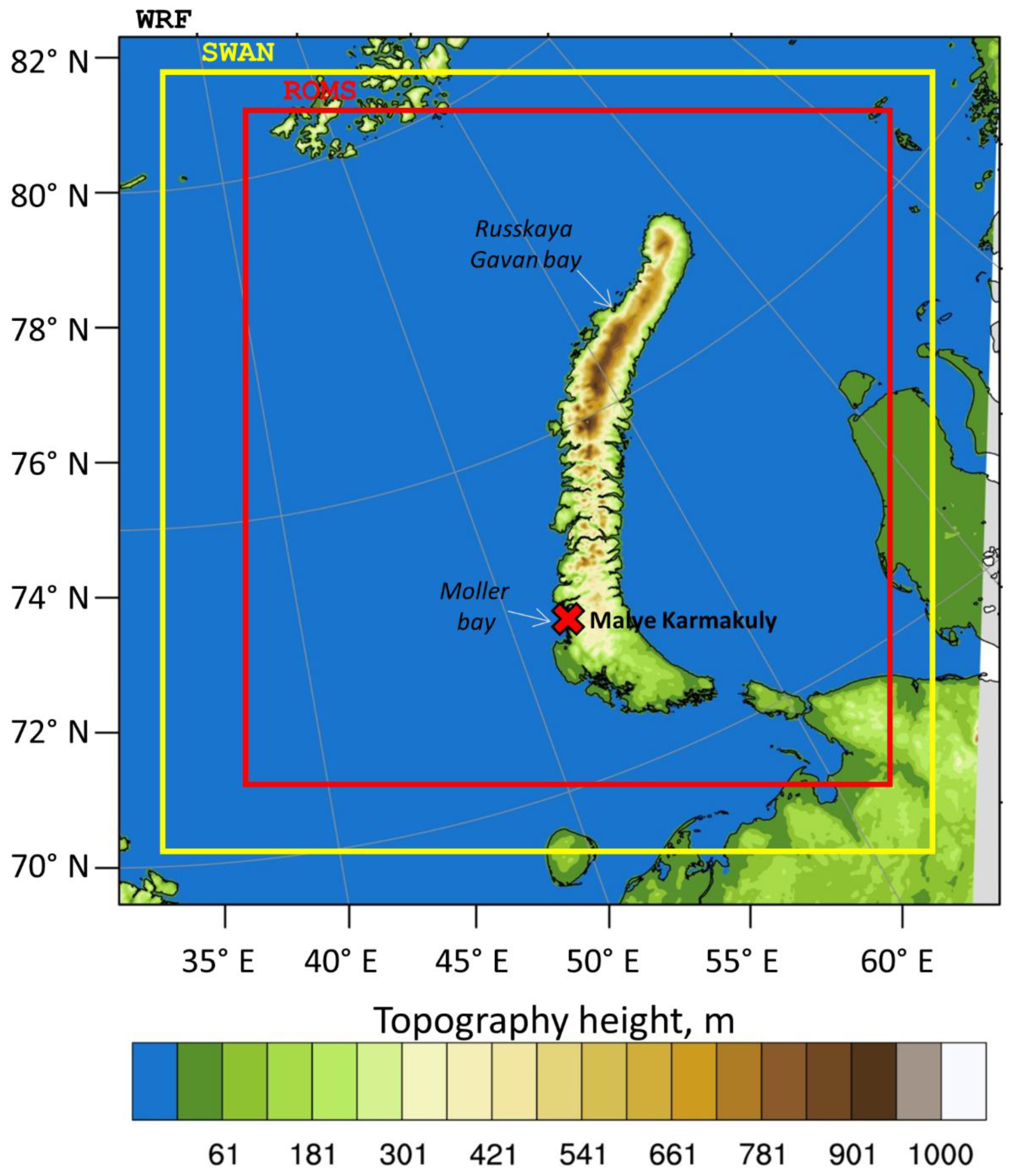
Coupled model domains: WRF (coincides with the boundaries of the map), SWAN (yellow rectangle) and ROMS (red rectangle). Color shows topography height (m). X-mark shows the location of the weather station.
2.5. Experimental Design
The model domains are shown in Figure 1. The WRF model domain with 460 × 480 horizontal grid nodes and 50 unevenly-spaced vertical levels covered most of the Barents and Kara Seas. The SWAN and ROMS domains were smaller than the atmospheric one to avoid sharp gradients at the boundaries. The horizontal grid spacing for all models was 3 km. The ROMS grid consisted of 333 by 363 horizontal grid nodes and 26 vertical levels with non-monotonic vertical resolution (grid spacing increased with depth). The SWAN grid had 404 × 424 grid nodes; spectral resolution was 10°. The coupling interval between models was set at 30 min. All experiments were started at 00 UTC 9 December and finished at 06 UTC 13 December 2006. The first day (9 December) was considered as a spin-up time and was excluded from the analysis. Table 1 summarizes the information about all the experiments.

Table 1.
List of experiments.
The control experiment “A” was run using only a stand-alone WRF model. Two experiments (“AO” and “AW”) represented two-way coupling of atmospheric model with the ocean and sea waves models, respectively. “AWO” is a fully three-way coupled simulation. Additional series of calculations were run to assess the sensitivity of the results to some parameters in a fully coupled mode. The “AWO Janssen” experiment used wave growth due to wind according to Janssen [62,63] (hereafter “Janssen”). It is based on a quasi-linear wind-wave theory and differs from “Komen” by explicitly accounting for the interaction of waves and wind. In the “Komen” parameterization, the drag coefficient is calculated according to a semi-empirical formula depending on the wind speed. In the “Janssen” parametrization, friction velocity is calculated iteratively based on wind speed and wave spectrum.
Another series of experiments tested the sensitivity of simulated results to the sea-surface roughness length parametrization. While the standard Charnock formula [64] was used in WRF when uncoupled with SWAN (“A” and “AO” experiments) and “Drennan” scheme was used in most of the coupled calculations, two other schemes was also tested in experiments “AWO Taylor_Yelland” and “AWO Oost”. As shown by a previous study [35], the “Drennan” parameterization in the Barents Sea conditions gives the smallest roughness length and turbulent momentum and heat fluxes of all the listed parameterizations. This parametrization also gives the smallest model bias in wind speed and SWH in the Barents Sea when compared with altimeter data (unpublished results). The drag coefficient constraint (2.85 × 10⁻³) for strong winds from [65], which is commonly used in tropical hurricane simulations, was used in all our SWAN runs.
While all these experiments were aimed at showing the sensitivity of turbulent heat exchange over the sea to coupling technique, the “AWO flat” experiment was designed to show the impact of bora itself on the heat fluxes and processes in the ocean. In this experiment, topography height was set to zero everywhere, simulating conditions of a simple cold-air outbreak under eastern winds without accounting for flow modifications by the orography. In some way, this experiment is an attempt to simulate a situation that could be found in a reanalysis with a very low resolution and thus with very smooth topography over NZ.
3. Results
3.1. Description of the Bora Eipsode and Model Verification
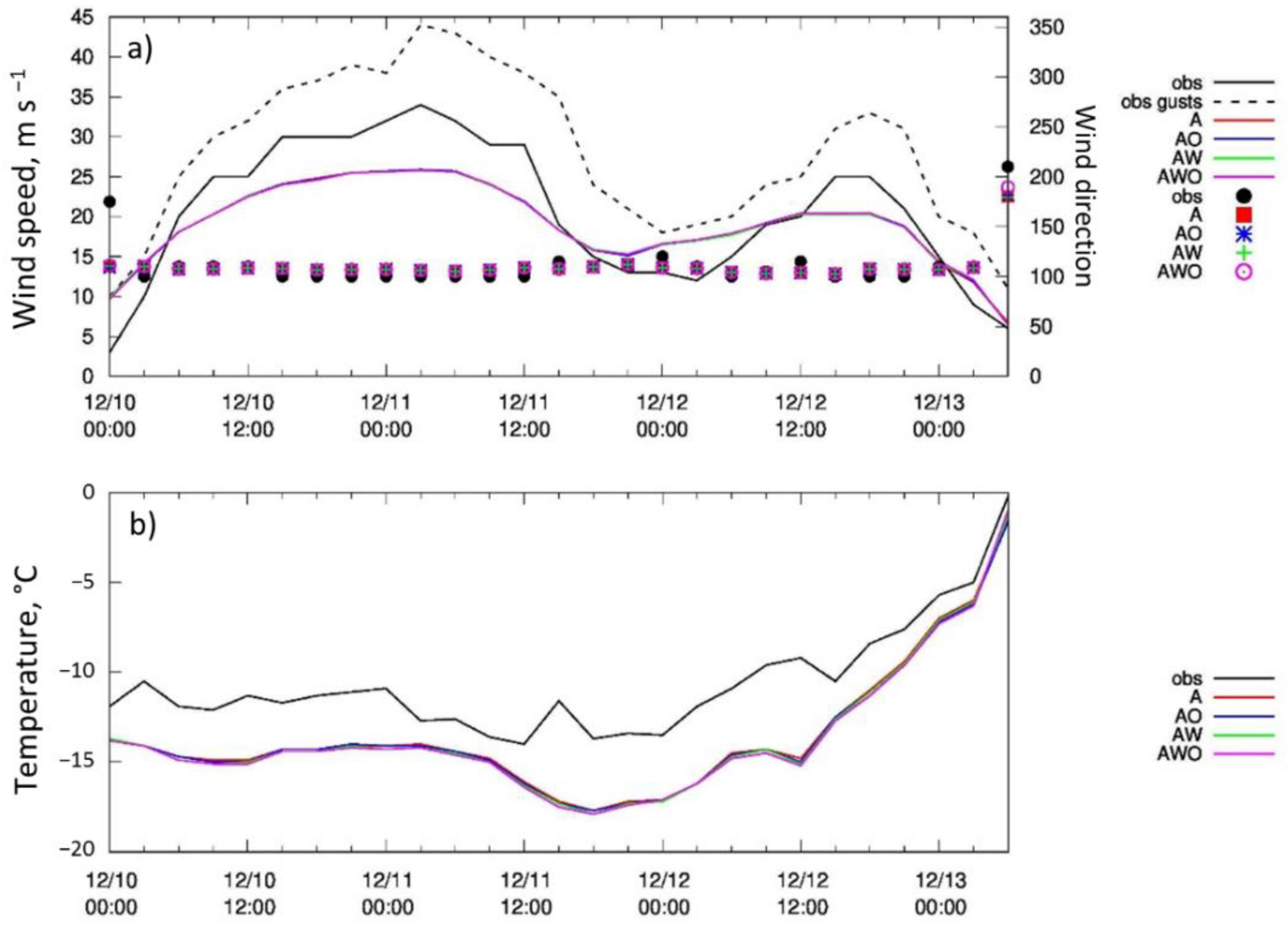
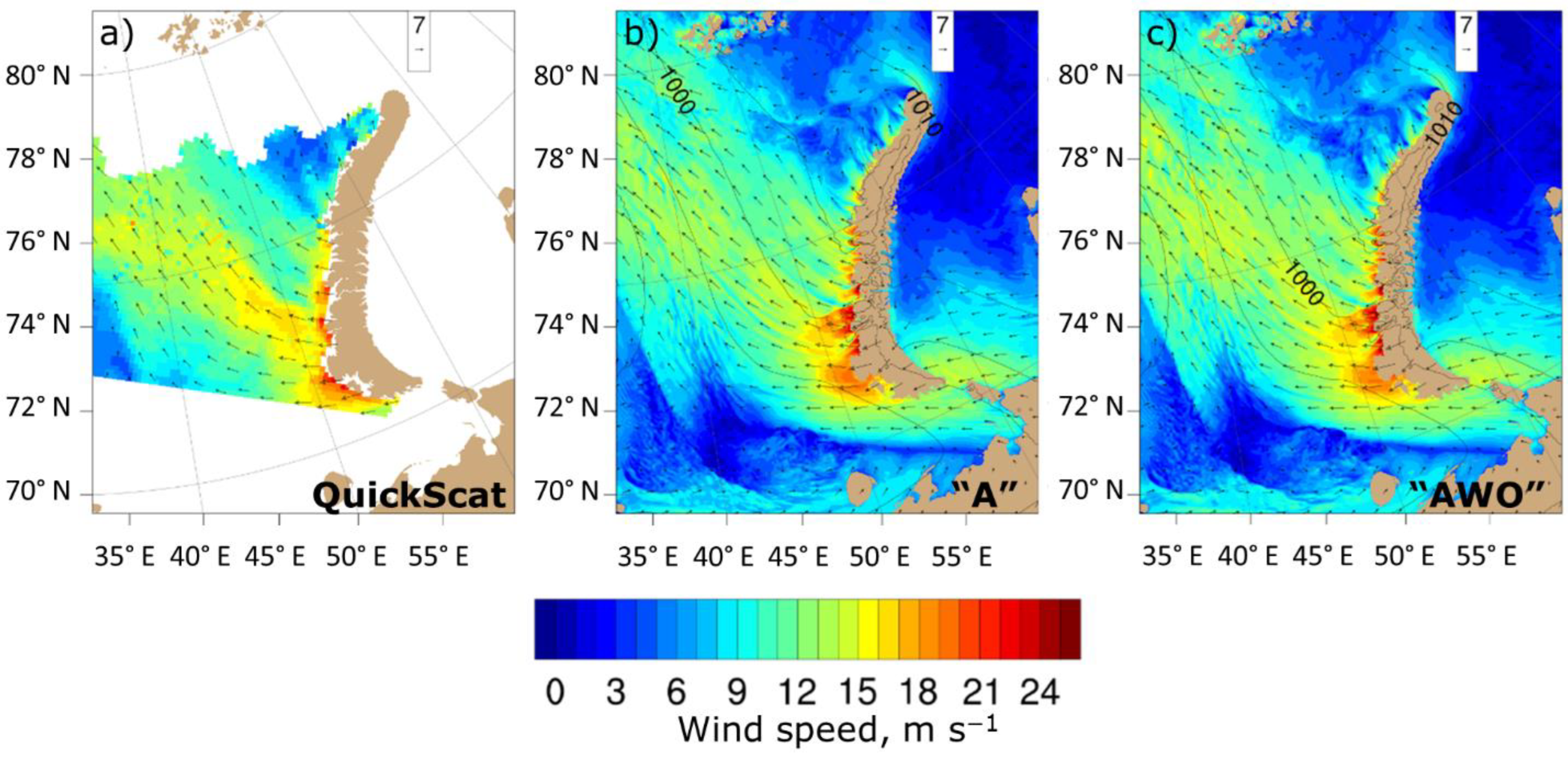
According to the Malye Karmakuly weather station, located on the southern island of Novaya Zemlya (Figure 1), bora was observed on 10–12 December 2006; the average 10-min wind speed attained 34 m s−1, and gusts reached 45 m s−1 (Figure 2a). An extensive cyclone, centered over the Greenland Sea, influenced the Barents Sea region during this period. It caused a rather strong (especially on 10 December) wind up to 15–20 m s−1 near the surface mainly of a southeasterly direction. All the numerical experiments reproduced the general course of the wind speed at the weather station; however, the maximum wind speeds did not reach the observed values (Figure 2a). This maximum wind speed underestimation is typical when modeling strong downslope windstorms in the Arctic with the WRF-ARW model [49]. The spatial distribution of wind speed during bora was well reproduced by the model (Figure 3) when compared with the QuickScat scatterometer data with a 12.5 km resolution. The mean model bias for the wind speed in the open sea was −1 m s−1 in experiments without simulating waves (“A” and “AO”) and about −0.5 m s−1 in experiments taking waves into account when compared with satellite altimeters Envisat, ERS and GFO (see pp. 2–4 in [66] for the description of these altimeter data archives); the mean absolute error was about 1.5 m s−1, and the correlation coefficient was 0.8 (Table 2). In general, the verification results indicate a satisfactory reproduction of the wind by the model, as well as the influence of wave accounting and the choice of roughness parameterization on the results of wind modeling (Table 2).
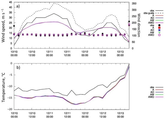
Figure 2.
10-m wind speed (solid lines), gusts (dashed line) and direction (markers) (a) and 2-m air temperature (b) from observations and simulations at the Malye Karmakuly weather station.
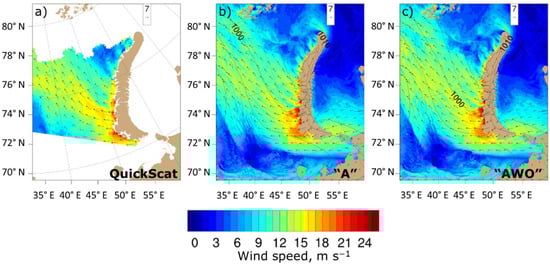
Figure 3.
Wind speed and direction from scatterometer data (a) and experiments “A” (b) and “AWO” (c) at 22 UTC on 10 December 2006. Grey contours show sea-level pressure (hPa).
Table 2.
Statistical characteristics of model errors in wind speed (m s−1) when compared with the altimeter data during the period 10–12 December 2006.
Novaya Zemlya bora can lead to both an increase and a decrease in air temperature [33], and consequently to different effects on turbulent heat fluxes. In this episode, the air temperature and relative humidity over the sea generally decreased compared to the ambient air not affected by the bora, which, in combination with high wind speed, should have led to an increase in turbulent heat fluxes from ocean to the atmosphere. The air temperature at Malye Karmakuly station was underestimated by the model by 2–5 °C. Nevertheless, preliminary model runs showed that the QNSE parametrization used in these experiments gives the closest values of wind speed and temperature to the observations compared to other boundary layer parametrizations.
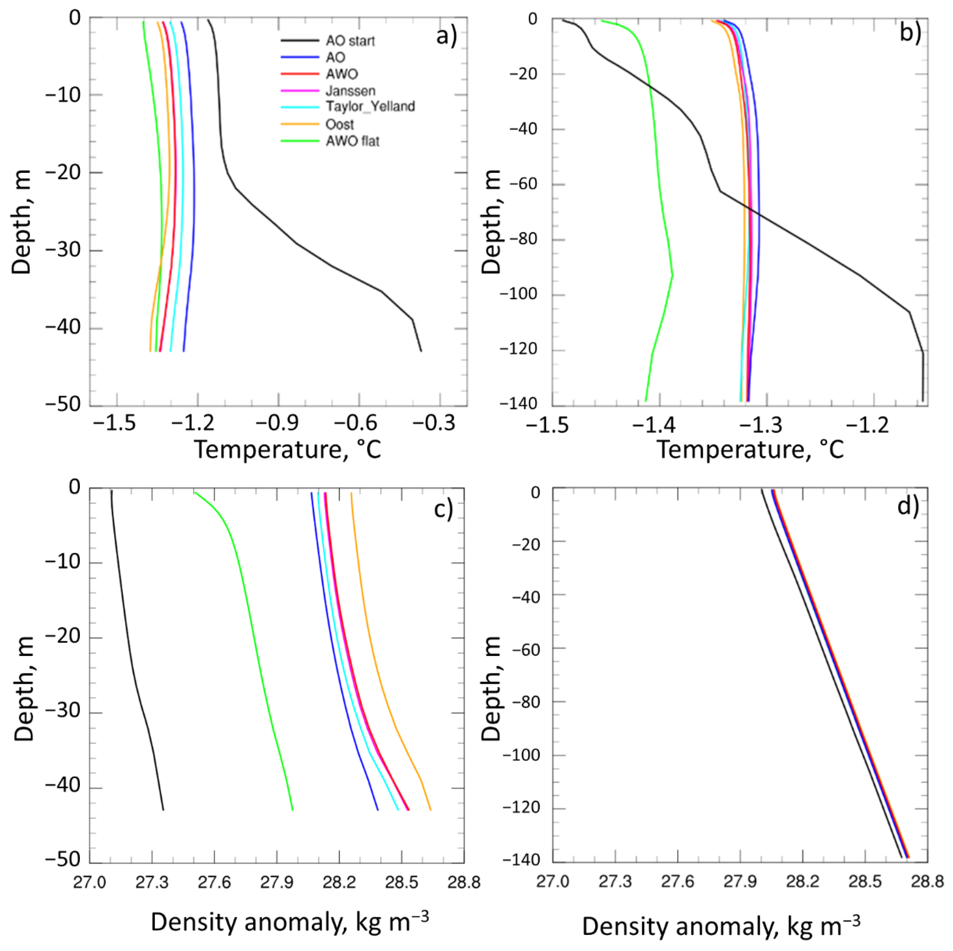
During this episode, ROMS simulated an increase in vertical mixing in the upper layer of the ocean. Intensive mixing in the open sea began even before the start of the bora and was caused by strong large-scale winds. The depth of the mixed layer downstream the southern part of the archipelago, in the open sea, increased during the experiments from 100 m to 200 m. Near the coast, the ocean mixed up to the bottom (Figure 4). In the southern part of the coast, the water temperature decreased more near the bottom (by almost 1 °C, Figure 4a), and in the northern part of the coast, the water temperature decreased at the bottom and slightly increased in the upper layer (by 0.1–0.2 °C), possibly due to the intervention of warmer water from below while mixing (Figure 4b). However, if we consider the change in water temperature (both surface and column-averaged) during the bora in the whole region, then it is quite difficult to detect any regularities. The field of temperature variation during the course of the simulation is quite patchy. This could be due to heterogeneity of heat fluxes in combination with different water density stratification in different areas, as well as due to the influence of ocean currents and sea ice, which significantly complicates interpretation.
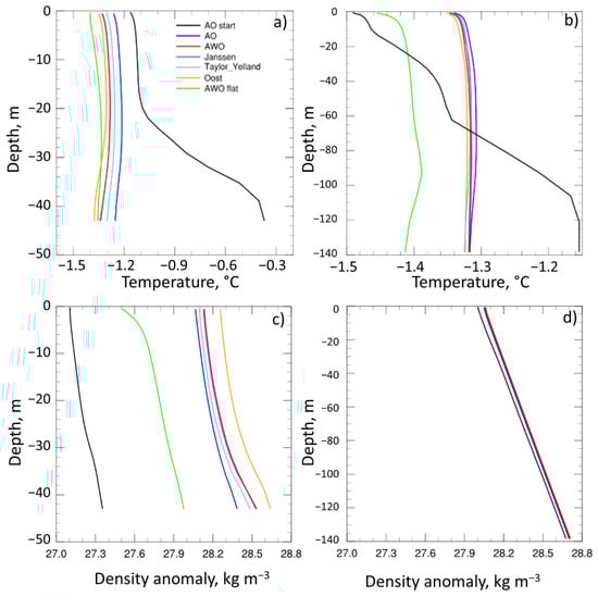
Figure 4.
Water temperature (a,b) and density anomaly (density “minus” 1000) (c,d) vertical profiles averaged in 15-km radius from the points (a,c) 72.3° N, 51.9° E and (b,d) 76.6° N, 63.6° E at the beginning (00UTC on 10 December, black line) and the end (18UTC on 12 December, colored lines) of bora in different experiments.
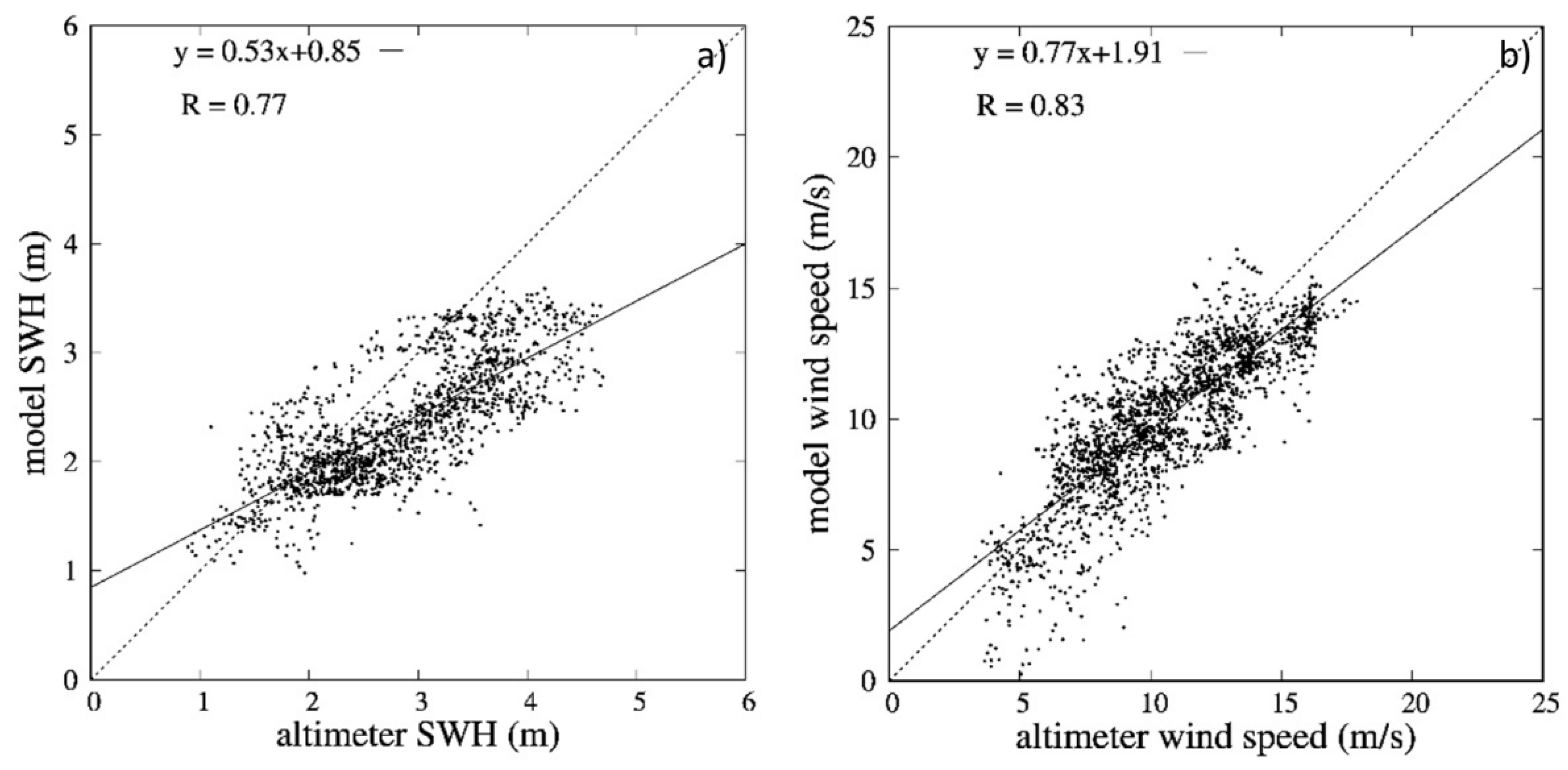
SWH during bora reached 2 m at a distance of 20 km from the coast, and 3.5 m at a distance of 50 km according to simulations. A faster growth of waves with distance from the shore was observed downstream of the fjords, where strong gap winds were blowing. Unlike a downslope windstorm, gap winds spread over a greater distance and decay more slowly. The steepest waves (with steepness up to 0.06–0.07), typical for bora [66], were simulated near the coast, at a distance of up to 15 km from the shore. In general, the model adequately reproduced SWH during this episode (Figure 5a) in comparison with the altimeter data (correlation coefficient 0.8). However, the bias (−0.5 m) and the root mean-square error (0.7 m) were quite large. The statistical characteristics of SWH model errors in all experiments were close except for “Taylor_Yelland” and especially “Oost” experiments, which were worse than others (Table 3).

Figure 5.
Scatter diagram of SWH (a) and wind speed (b) from altimeter data and simulation results (“AWO” experiment). Regression line, regression equation and correlation coefficient are also shown.
Table 3.
Statistical characteristics of model errors in SWH (m) when compared with the altimeter data during the period 10–12 December 2006.
The dynamics of sea ice were also simulated. The largest changes in the position of the sea ice edge occurred in the north and northeast of the Barents Sea (the edge moved slightly to the north). These changes are consistent with the AMSR-E satellite ice observations. Some new ice has formed in Moller Bay (see Figure 1) and near the northern part of the NZ coast according to the model. The sea ice near the central part of the NZ coast was carried northward by a strong coastal current, and part of this ice melted. In general, most of the western coast of Novaya Zemlya was covered by fragmentary sea ice. Due to the coarse resolution of the satellite data, it was difficult to verify the simulated ice dynamics in the coastal region.
3.2. Impact of Model Coupling on Turbulent Fluxes
The turbulent heat fluxes averaged over the whole NZ region were almost the same in “A” and “AO” experiments (Table 4). The expected effect of the decrease in heat fluxes due to SST cooling with online interaction between atmosphere and ocean appeared only in a narrow zone near the coast (Figure 6b). The field of heat fluxes difference followed the field of water temperature anomaly in the “AO” experiment. The latter was determined by many factors, heat advection with currents and sea ice thermodynamics among them. The ocean-atmosphere coupling has also a zero effect on the momentum flux (Table 4, Figure 7b).
Table 4.
Average differences in sensible (H), latent (LE) and total (H+LE) heat fluxes (W m−2), momentum flux τ (N m−2) and wind speed U10 (m s−1) between experiments in the NZ region. The relative differences are indicated in brackets, rounded to integers (in %). The region of averaging coincides with the region shown in Figure 6, Figure 7 and Figure 8, areas with sea ice were excluded.
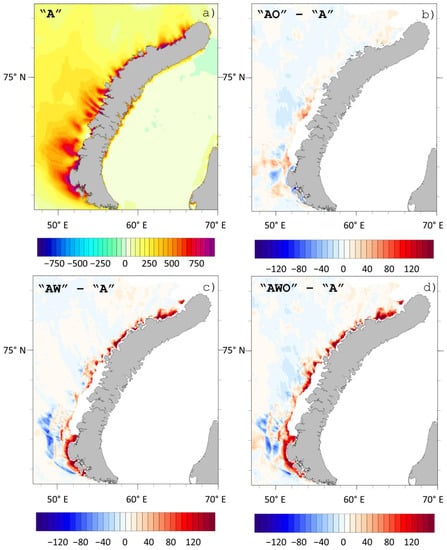
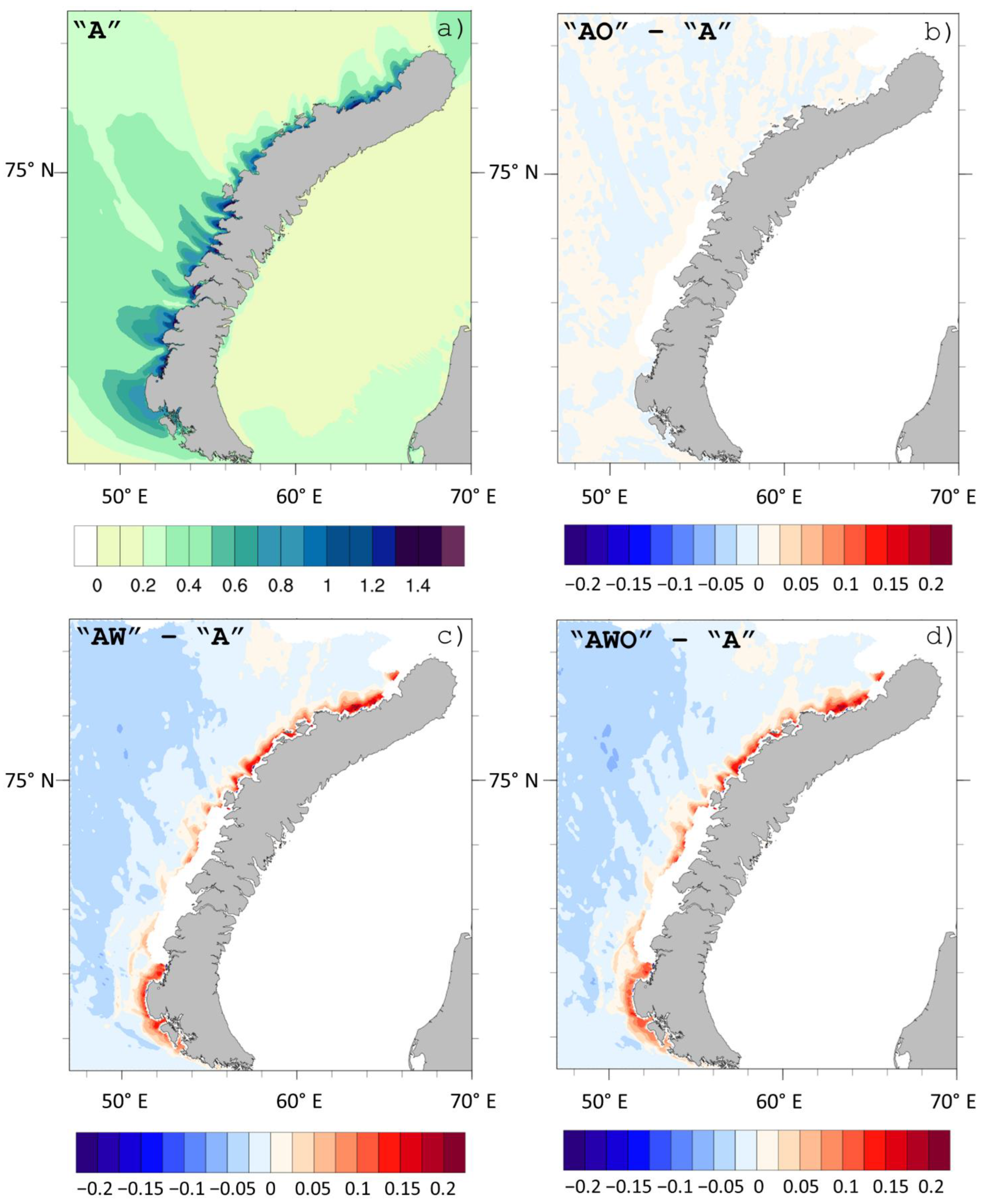
Figure 6.
Total turbulent heat flux (W m−2) in experiment “A” (a) and difference in heat fluxes (W m−2) between coupled experiments “AO” (b), “AW” (c), “AWO” (d) and uncoupled experiment “A” averaged over the bora period (10–12 December). Areas with sea ice from experiment “A” in (b–d) are shaded in white.
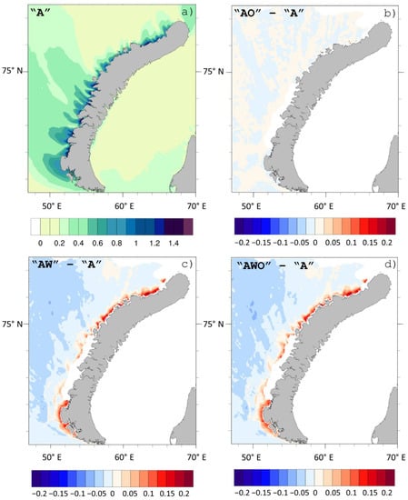
Figure 7.
Momentum flux (N m−2) in experiment “A” (a) and difference in momentum fluxes (N m−2) between coupled experiments “AO” (b), “AW” (c), “AWO” (d) and uncoupled experiment “A” averaged over the bora period (10–12 December). Areas with sea ice from experiment “A” in (b–d) are shaded in white.
In experiments with the wave model coupled with the atmospheric model, the heat and momentum fluxes increased near the coast (Figure 6 and Figure 7c,d) due to an increase in the drag coefficient compared with the uncoupled experiment. The drag coefficient, calculated as , was 2 − 2.2 × 10⁻³ in experiment “A” and 2 − 2.4 × 10⁻³ in experiments “AW” and “AWO” near the coast (Figure 8). The increase of drag coefficient near the coast and its decrease in the open sea when using the “Drennan” parameterization compared to the standard Charnock scheme was caused by the dependence of the former on the inverse wave age. Offshore wind causes young waves near the coast with the wave age increasing with fetch (distance from shore). The decrease of the drag coefficient in the open sea in “AW” and “AWO” experiments compared to “A” experiment occurred over a large area and, in total, outweighed the effect of drag increase near the coast, so the spatially-averaged momentum flux anomaly is negative (Table 4). Such a decrease in drag coefficient compared to the Charnock scheme is typical for the “Drennan” parameterization, at least in the Barents Sea conditions [35]. The same remark applies to the wind speed: it decreased near the coast, where the drag coefficient increased, but its average anomaly is positive (Table 4).

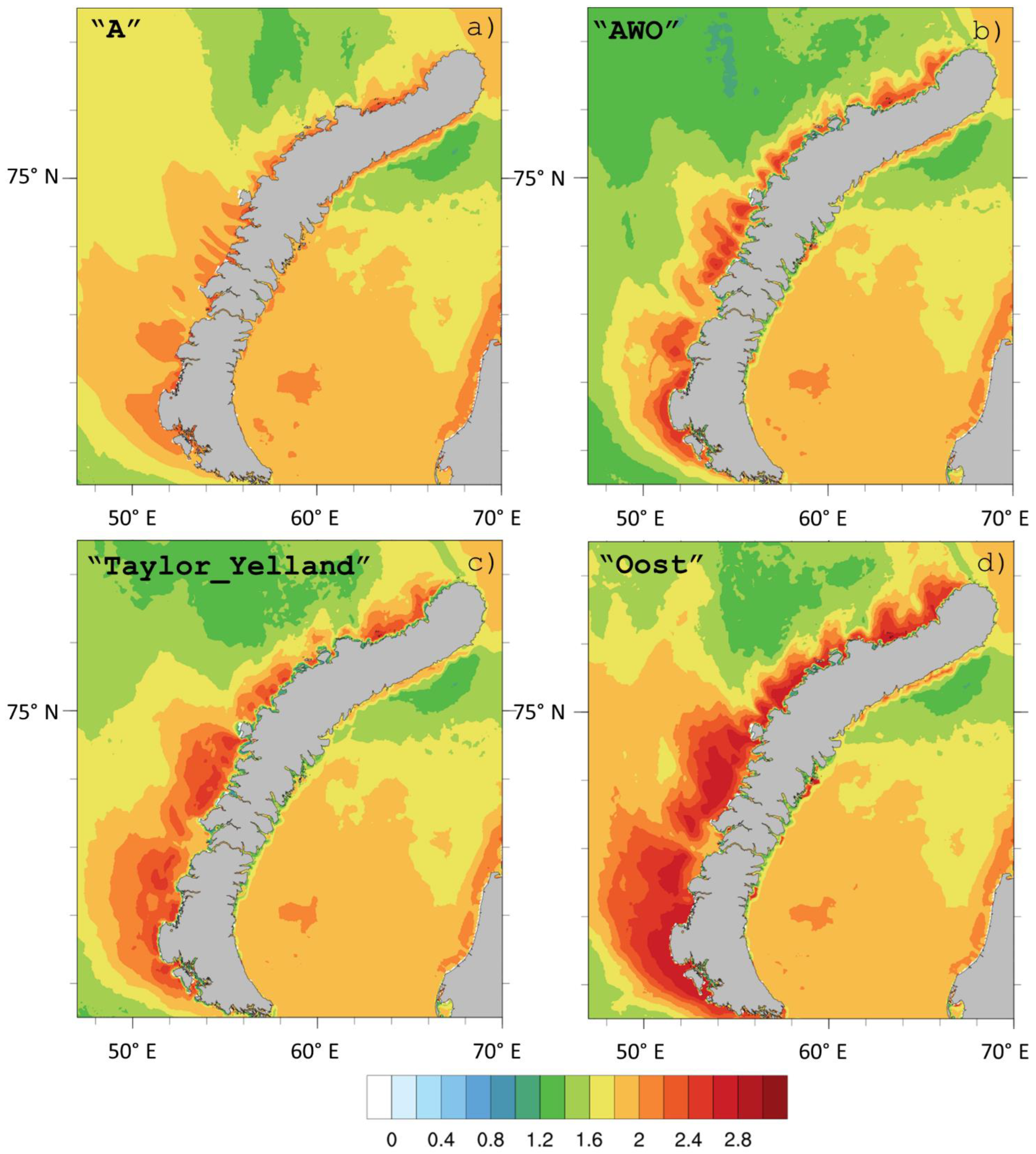
Figure 8.
Drag coefficient (×103) in experiments “A” (a), “AWO” (b), “Taylor_Yelland” (c) and “Oost” (d), averaged over the bora period (10–12 December).
In the “AWO” experiment, the effects of sea waves and ocean added up and the average anomaly of turbulent heat fluxes compared to “A” experiment was 7 W m−2 (or 3% of the fluxes magnitude in experiment “A”) (Table 4). The effect of SST cooling due to air-ocean interaction was smaller than the effect of increased sea surface roughness due to air-sea-waves interaction, so the heat fluxes anomaly in the “AWO” experiment was positive everywhere near the coast (up to 100 km from the shore) (Figure 6d). In some areas, the positive relative heat flux anomaly exceeded 50% of the heat flux magnitude (for example, near Russkaya Gavan Bay (see Figure 1)). The maximum heat flux anomaly attained 1000 W m−2.
In fact, the effects of the ocean and sea waves did not simply add up in the “AWO” experiment, but there was also a slight shift of the heat fluxes positive anomaly edge away from the coast (by about 5 km). This was due to wave-current interaction, which results in a Doppler shift (product of wave number and current velocity) in the wave frequency (up to 0.2 s−1 near the coast) and a change in their phase velocity. The phase velocity of the waves ranged from 5 m s−1 near the coast to 13 m s−1 in the open sea, while the velocity of the surface current ranged from 1 m s−1 near the coast to 0.1 m s−1 in the open sea. In the “AWO” experiment, the phase velocity mainly decreased (by up to 1 m s−1) compared to the “AW” experiment, which led to a decrease in the wave age (which is the ratio of the phase velocity to the friction velocity) and, consequently, to surface roughness increase according to the “Drennan” formulation. However, this effect is small in terms of spatially-averaged heat fluxes.
The influence of wind input parameterization in SWAN (“Komen” and “Janssen”) on the average heat and momentum fluxes was small (Table 4). On the contrary, the choice of roughness parameterization had a significant impact. The “Taylor_Yelland” parameterization gave higher drag coefficient values near the coast and in the open sea compared to the “Drennan” parameterization (Figure 8b,c), although on average the differences in heat fluxes between these parameterizations were small (Table 4). The “Oost” parameterization gave higher values of both the drag coefficient (Figure 8d) and the heat and momentum fluxes near the coast and in the open sea; the difference between the “Oost” and “A” experiments was on average 6–7% (Table 4), and the wind speed decreased everywhere compared to experiment “A”. It is worth nothing that the “Oost” experiment showed the worst fit to observed altimeter wind speed and SWH data (Section 3.1).
3.3. Impact of Bora on Turbulent Fluxes and Ocean Processes
In this section, the results of the “AWO flat” and “AWO” experiments are discussed. The latter is considered the control, i.e., the experiment in which bora is reproduced. As shown above, the influence of roughness parameterizations was strong, but the “AWO” experiment with “Drennan” parametrization was more accurate than “Taylor_Yelland” and “Oost” experiments, according to the results of verification with altimeter data.
The total turbulent heat fluxes, on average over the region, were significantly lower (by 18%) when bora is taken into account than in the flat experiment (Table 4). The exception is the narrow coastal zone, where the bora enhanced the fluxes. It is known that bora is very strong near the shore, but quickly weakens over the sea due to friction or a hydraulic jump (when jet stream decouples from the surface). As a result, a wake is usually forming at some distance from the shore. This wake was clearly seen downstream from the northern island of NZ (Figure 3), where mountains are higher and hydraulic jump and other nonlinear effects are more pronounced. This region of the wind wake during bora occupied a larger area than the region of high wind speeds. Thus, the presence of orography redistributes the wind field and, when averaged over the whole region, this led to a weakening of turbulent heat fluxes in the “AWO flat” experiment compared to the “AWO” experiment, although the momentum flux, on average, increased due to the very high speed of bora winds.
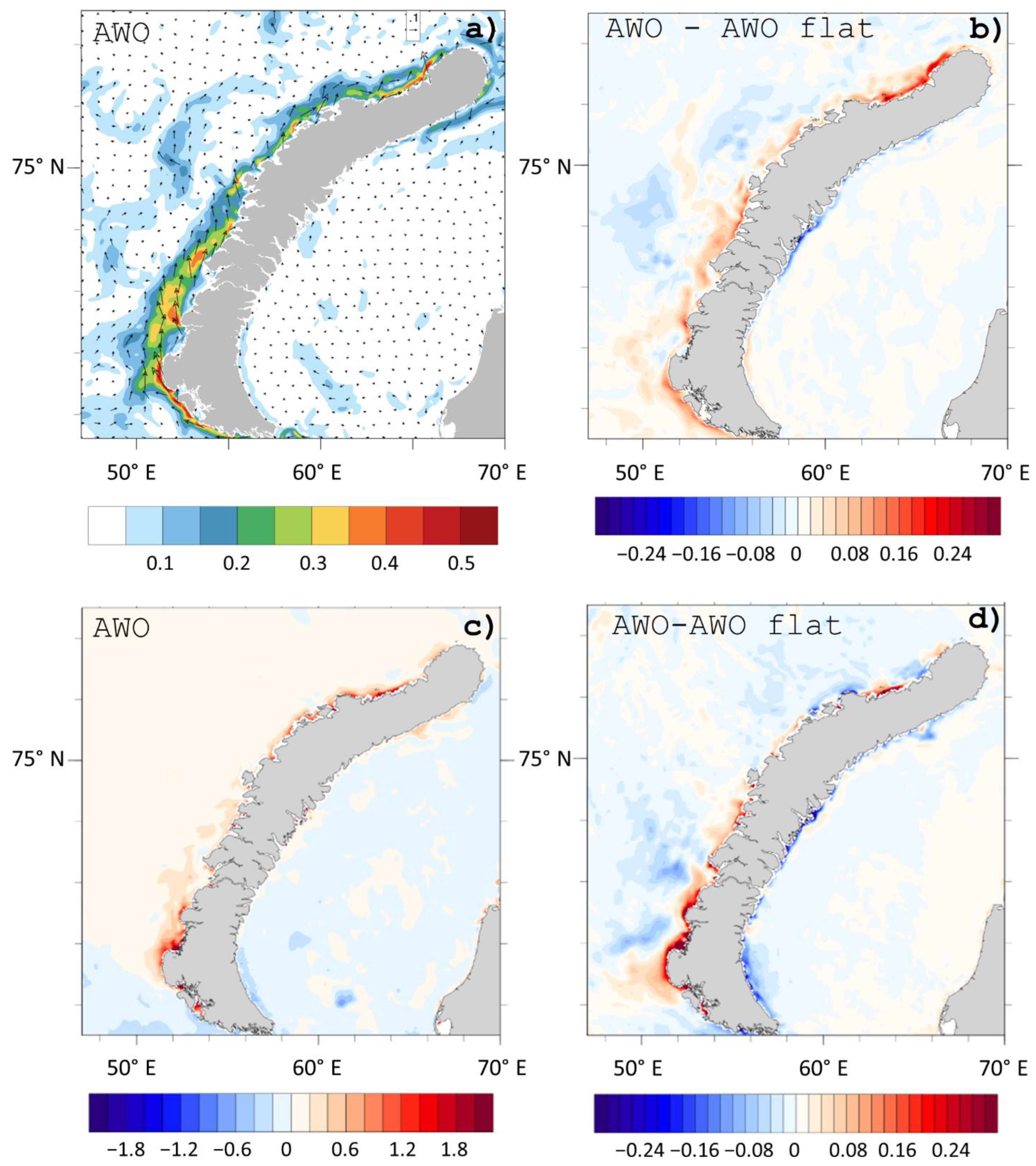
Qualitatively, the pattern of ocean currents was similar in experiments with and without bora. In both experiments, a strong southern coastal current developed along the western coast of NZ (Figure 9a). In the “AWO” experiment, the current in the northern part of NZ coast was more pronounced and stronger than in the “AWO flat” experiment (Figure 9b). The depth-averaged current velocity in the “AWO” experiment was higher by 0.1–0.15 m s−1 in the southern and central parts of the NZ coast and by 0.2–0.25 m s−1 in the northern part (the maximum difference there reached 0.5 m s−1) compared to the “AWO flat” experiment. Surface current direction approximately coincided with the wind direction and its velocity reached 0.9 m s−1 in the “AWO” experiment. Such velocities are not unbelievable: there are known cases of the bora-caused drift of icebergs (that have broken off from NZ outlet glacier) at a speed of more than 0.75 m s−1 [67].

Figure 9.
Depth-averaged current speed (m s−1) (a), difference in current speed (m s−1) between “AWO” and “AWO flat” experiment (b), change of water density (kg m−3) during bora (c) and difference in water density (kg m−3) between “AWO” and “AWO flat” experiments (d) averaged over the bora period (10–12 December).
As mentioned in the introduction, the western coast of NZ is a source of dense water during the cold season. The simulation results revealed water densification along the NZ coast during bora (Figure 9c), caused by salinization due to brine release during the ice formation and enhanced evaporation and to a lesser extent by water cooling during heat exchange with the atmosphere. Densification in most parts of the coast was stronger in the experiment with bora than in the flat experiment (Figure 4c and Figure 9d), mainly due to stronger evaporation (although in some places the changes were associated with differences in sea ice dynamics in these two experiments). The water salinity near the coast in the southern part reached 35.5, and the density was 1029 kg m−3 in “AWO” experiment, while salinity did not exceed 34.5 (less than the typical value for Arctic Intermediate Water), and the density was 1028 kg m−3 in the “AWO flat” experiment. In the “AWO” experiment, dense water was concentrated at the bottom.
In the SODA reanalysis, water temperature near the coast decreased (comparing the average of 10–14 December with the average of 4–9 December), and the depth of the mixed layer increased (although it did not reach the bottom, in contrast to simulations). However, the salinity near the coast was much lower (about 33.5) and remained almost the same through all this period. In the absence of direct observations of salinity in this area, it is impossible to judge which salinity value was correct, but given the known fact that dense waters form off the coast of NZ during strong winds [34], our simulation results seem more plausible.
In the “AWO” experiment, the ocean lost about 3% of its heat content during the bora episode, while in the flat experiment, the ocean lost 0.5% (or 12 MJ m−2) more. Downstream the northern part of NZ, where the wind wake and the positive air temperature anomaly were most pronounced in the “AWO” experiment, and locally downstream the central and southern parts, the average ocean heat content during bora was higher in the “AWO” experiment than in the “AWO flat” (Figure 10). Figure 4 also demonstrates that ocean downstream the northern island and partly downstream the southern island was the coolest in the flat experiment. Thus, orography and orographic winds save heat in the ocean, concentrating heat losses near the coast (where the heat content is small), and decreasing turbulent heat transfer from the ocean to the atmosphere in wakes. It could also be noted from Table 5 that the differences between experiments discussed in the previous section (even the experiments with different roughness parametrizations) are small in terms of ocean heat content.

Figure 10.
Difference in ocean heat content (MJ m−2) between “AWO” and “AWO flat” experiment averaged over the bora period (10–12 December).
Table 5.
Differences in ocean heat content ΔOHC (MJ m−2) between the bora end (06UTC on 13 December) and bora beginning (06UTC on 10 December) averaged over the region 45–70° E, 71–77.5° N (excluding areas with sea ice). The relative differences are indicated in brackets (in % of the heat content at the bora beginning OHC1).
Figure 11 shows the water temperature cross-section through the central part of NZ and confirms that the influence of orography on the ocean heat content in the open sea is generally small. A remarkable feature in the eastern Barents Sea is the presence of Atlantic water with high temperature and salinity. Atlantic water is clearly visible in Figure 11 as a warm spot at a depth of 120 m with a temperature of up to 3.5 °C (according to the SODA reanalysis data for 5–9 December) at a distance of about 250 km from the NZ coast. After 5 days, the temperature in SODA reanalysis slightly decreased (Figure 11b), but not as much as in simulations (Figure 11c,d). In both experiments (“AWO “and “AWO flat”), the temperature of the Atlantic water decreased by almost 1 °C and, in general, the depth of the mixed layer increased. Differences between the experiments are small. Differences between the reanalysis and simulation results are probably due to the difference in atmospheric forcing: the MERRA2 atmospheric reanalysis with a rather coarse resolution was used in SODA reanalysis. The wind speed and turbulent fluxes are usually lower and consequently the ocean heat loss is smaller in the coarse-resolution reanalyses than in high-resolution simulations.

Figure 11.
Cross-section of water temperature (°C) across 74.1° N in SODA reanalysis for 7 December (average over 5–9 December) (a), for 12 December (average over 10–14 December) (b) and in “AWO” (c) and “AWO flat” (d) experiments at the bora end (18 UTC 12 December).
The cross-sections of turbulent kinetic energy (TKE) in the south and north of NZ (Figure 12) confirm that the influence of bora does not extend far into the sea. Near the coast, TKE in the “AWO” experiment is higher than in the “AWO flat” experiment. At a distance from the shore in the southern cross-section, the differences between the experiments are small, since the height of the mountains in the south of NZ is small and the wind wake in this case is not as strong as downstream the northern island. In the north, there is absolutely no mixing in “AWO” experiment due to the wake.
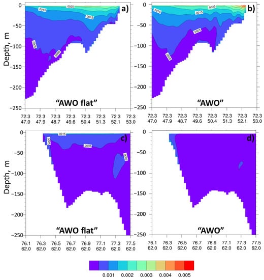
Figure 12.
Cross-section of TKE (m2 s−2) along 72.3° N (a,b) and 62° E (c,d) in “AWO flat” (a,c) and “AWO” (b,d) experiments.
4. Discussion and Conclusions
Numerical experiments with the COAWST coupled model for one winter episode of strong Novaya Zemlya bora (10–12 December 2006) were aimed at estimating the role of the ocean-atmosphere interaction in energy exchange at the sea surface under bora conditions and the role of bora in ocean processes. Below the main results are summarized:
- When the interaction between the atmosphere and sea waves is taken into account, turbulent heat exchange increases (on average by 3%) due to an increase in the roughness coefficient near the coast (up to 100–150 km from the coast) caused by young steep waves.
- When the interaction of the atmosphere and the ocean is taken into account, the turbulent heat exchange averaged over the region does not change compared to the control experiment. SST cooling was found only in a narrow strip near the coast, while the difference in SST between the control and “AO” experiments is multidirectional elsewhere. This could be due to complexity of processes determining water temperature, such as heat advection with currents, heat release and consumption of sea ice freezing/melting.
- When both ocean and wave models are coupled with the atmospheric model, the above effects of ocean and sea waves add up and we see two zones where (1) fluxes increase due to rough waves on a distance of up to 100 km from the shore and (2) the effect of coupling on fluxes is generally small in the open sea. In this fully coupled run, the effect of decreased heat fluxes due ocean cooling near the coast is overwhelmed by the greater increase of roughness (and turbulent fluxes, consequently) due to sea waves.
- Bora reduces the turbulent heat exchange between the ocean and the atmosphere (compared to similar conditions in the absence of bora) by 18% on average over the region, although in the coastal region, heat transfer locally increases by 50–150%.
- Bora intensifies ocean current along the western coast of Novaya Zemlya by 0.1–0.25 m s−1 on average
- Orography of NZ and orographic winds conserve heat in the ocean. The average ocean heat content in this region decreased by 2.7% during bora, but it decreased even more in the flat experiment
- Since the direct influence of bora winds extends only to the coastal zone, bora does not directly affect the mixing of the Atlantic water, since it flows too far from the coast.
- Salinization (due to increased evaporation and formation of new ice during bora) and, to a lesser extent, cooling of coastal waters leads to a strong water densification. In the flat experiment, this densification is weakened, and the water density is noticeably lower than the density of the Arctic Intermediate Water. Thus, bora clearly contributes to the formation of dense waters on the NZ shelf, and accounting for bora is necessary for a correct assessment of this process. Water densification was also revealed during the Adriatic bora [68]; however, only the effect of model coupling, but not the bora itself, on densification has been considered. Summarizing, when modeling the ocean and sea ice to study the formation of bottom waters near Novaya Zemlya with coarse-resolution atmospheric forcing (as, for example, in [69]) one should be careful about the resulting estimates.
All the expected processes associated with the air-sea interaction (see the Introduction) were found in our simulations, though with some deviations. For example, the effect of atmosphere-ocean models coupling on heat fluxes turned out to be small on average. Some effect of currents and sea waves interaction was found, though also small. We did not found any significant influence of bora on the Atlantic water. There is no direct influence of bora wind in the open sea, since the horizontal scale of bora does not exceed 100 km. However, bora as a phenomenon as a whole—including the formation of a wind wake, as well as the adiabatic heating of the descending air, which spreads over a long distance (e.g., [70])—largely determines the atmosphere-ocean energy exchange and ocean mixing, especially downstream the northern more mountainous part of NZ. Bora has a significant impact on the processes in the ocean directly near the coast—coastal currents and especially formation of dense waters.
The main limitations of this study are the following. First of all, the reliability of the conclusions obtained using the modeling results could not be proved due to the lack of ocean in-situ observation. Secondly, the obtained modeling errors of wind speed and significant wave height (when verifying against the altimeter data and Malye Karmakuly weather station) are quite large. Therefore, the flux estimates obtained here arenot accurate. Thus, the emphasis of this work was not on the absolute values of the fluxes, but on the differences between the experiments.
For the same reason (lack of coastal offshore observations), we cannot reliably determine whether the coupled model reproduces the processes in the atmosphere and ocean near the coast better or worse than the uncoupled model. Comparison of wind speed and temperature at the Malye Karmakuly station did not reveal any differences between coupled and uncoupled models. Nevertheless, at least in the open sea, the coupling of the atmospheric and sea wave model using the Drenan et al. (2003) roughness parametrization gives a smaller error in the wind speed compared to a stand-alone atmospheric model and compared to the coupled simulations with other roughness parameterizations.
In addition, there is a known problem of the applicability of standard theories and parametrizations under coastal wind conditions. For example, this study uses the roughness length upper limit for strong winds [65]. This constraint is commonly used in hurricane simulations, since too high drag prevents the hurricane development to the observed intensity. However, the issue of using this limit in the conditions of coastal winds, though very strong, remains open. For instance, observations of atmospheric turbulence on the offshore platform in Katsiveli (Crimea) on the Black Sea coast show that even with a wind of 15 m s−1 directed from the shore, the drag coefficient exceeds 3 × 10⁻³, and with winds from the sea, the drag is much less [71]. The Monin–Obukhov similarity theory is generally not applicable when there are offshore winds because internal boundary layers form due to a sharp change in surface roughness between land and sea. In the first kilometers offshore, there is strong advection of turbulence from land at some height over the sea (e.g., [72]), while the lowest layer near the surface usually is adjusted to the sea surface roughness. Thus, even if observations of turbulent fluxes in the coastal region are available, it is not entirely clear how they can be compared with the simulation results.
We performed the flat experiment to find out the importance of accurately taking into account orography and bora winds on heat flux estimates and to assess whether the flux estimates obtained from the low-resolution reanalysis are correct. However, the “AWO flat” high-resolution experiment cannot be associated with low-resolution reanalyses, since the latter smooth the wind speed (and consequently the turbulent fluxes) not only in mountainous areas due to poor orography representation, but also in the open sea [73,74] due to poor representation of extreme values. We calculated the difference in the total heat flux averaged over the same area and over the same time period between different reanalyses and the “AWO” experiment. The difference for the DOE reanalysis [75] with ~1.9° horizontal resolution is −13%, a similar difference is −83% for the ERA-Interim reanalysis [76] with ~0.7° resolution and −29% for the CFSR reanalysis [77] with 0.5° resolution. Thus, the highest average turbulent heat fluxes in different reanalyses are lower than in the “AWO” experiment, while in the “AWO flat” experiment, they are higher than in the “AWO” experiment. Therefore, it would be better to perform simulation with coarse resolution rather than with flat topography, if the adequacy of reanalyses heat fluxes are investigated.
Finally, a major limitation of the work is that only one bora episode was simulated. More episodes are planned to be simulated to validate the results obtained in this study.
Author Contributions
Conceptualization, Methodology, Formal Analysis, Writing, Visualization—A.A.S., Software—A.A.S. and A.V.D. All authors have read and agreed to the published version of the manuscript.
Funding
This research was funded by the Russian Science Foundation (grant no. 18-77-10072) and in part (coupling of COAWST and ROMS ice model) by Russian Ministry of Science and Higher Education (agreement No. 075-15-2019-1621).
Institutional Review Board Statement
Not applicable.
Informed Consent Statement
Not applicable.
Data Availability Statement
The COAWST modeling system is distributed freely via github (https://github.com/jcwarner-usgs/COAWST (accessed on 10 July 2022)). The ERA5, ASR v2, ERA-Interim, DOE, CFSR reanalyses and GFS FNL analysis were downloaded from NCAR Research Data Archive (https://rda.ucar.edu (accessed on 10 July 2022)). The SODA reanalysis is available at https://www.soda.umd.edu/ (accessed on 10 July 2022). AMSR-E/Aqua daily sea ice concentration and snow depth with 12.5-km resolution is available at https://nsidc.org/data/AE_SI12/versions/3 (accessed on 10 July 2022). TPXO tides data is available to registered users at https://www.tpxo.net/home (accessed on 10 July 2022). ETOPO2 database is available at https://www.ngdc.noaa.gov/mgg/global/etopo2.html (accessed on 10 July 2022). QuikSCAT Level 2B version 3.1 ocean wind vectors with 12.5 km resolution are available at https://podaac.jpl.nasa.gov/dataset/QSCAT_LEVEL_2B_OWV_COMP_12_LCR_3.1 (accessed on 10 July 2022).
Acknowledgments
The authors thank I.A. Repina, D.G. Chechin and P.A. Toropov for fruitful discussions of the results and J. Warner for technical help.
Conflicts of Interest
The authors declare no conflict of interest.
References
- Giorgi, F.; Gao, X.J. Regional earth system modeling: Review and future directions. Atmos. Ocean. Sci. Lett. 2018, 11, 189–197. [Google Scholar] [CrossRef] [Green Version]
- Aldrian, E.; Sein, D.; Jacob, D.; Gates, L.D.; Podzun, R. Modelling Indonesian rainfall with a coupled regional model. Clim. Dyn. 2005, 25, 1–17. [Google Scholar] [CrossRef]
- Wei, J.; Malanotte-Rizzoli, P.; Eltahir, E.A.B.; Xue, P.; Xu, D. Coupling of a regional atmospheric model (RegCM3) and a regional ocean model (FVCOM) over the maritime continent. Clim. Dyn. 2014, 43, 1575–1594. [Google Scholar] [CrossRef] [Green Version]
- Holt, T.; Cummings, J.A.; Bishop, C.H.; Doyle, J.D.; Hong, X.; Chen, S.; Jin, Y. Development and testing of a coupled ocean–atmosphere mesoscale ensemble prediction system. Ocean Dyn. 2011, 61, 1937–1954. [Google Scholar] [CrossRef]
- Ricchi, A.; Miglietta, M.M.; Falco, P.P.; Benetazzo, A.; Bonaldo, D.; Bergamasco, A.; Sclavo, M.; Carniel, S. On the use of a coupled ocean–atmosphere–wave model during an extreme cold air outbreak over the Adriatic Sea. Atmos. Res. 2016, 172, 48–65. [Google Scholar] [CrossRef]
- Sitz, L.E.; Di Sante, F.; Farneti, R.; Fuentes-Franco, R.; Coppola, E.; Mariotti, L.; Reale, M.; Sannino, G.; Barreiro, M.; Nogherotto, R.; et al. Description and evaluation of the Earth System Regional Climate Model (Reg CM-ES). J. Adv. Model. Earth Syst. 2017, 9, 1863–1886. [Google Scholar] [CrossRef]
- Kumar, P.; Mishra, A.K.; Dubey, A.K.; Javed, A.; Saharwardi, M.; Kumari, A.; Sachan, D.; Cabos, W.; Jacob, D.; Sein, D.V. Regional earth system modelling framework for CORDEX-SA: An integrated model assessment for Indian summer monsoon rainfall. Clim. Dyn. 2022, 1–20. [Google Scholar] [CrossRef]
- Bruneau, N.; Toumi, R. A fully-coupled atmosphere-ocean-wave model of the Caspian Sea. Ocean Model. 2016, 107, 97–111. [Google Scholar] [CrossRef]
- Di Sante, F. Assessing the role of local air–sea interaction over the South Asia region in simulating the Indian Summer Monsoon (ISM) using the new earth system model RegCM-ES. In Proceedings of the 19th EGU General Assembly, Vienna, Austria, 23–28 April 2017; p. 2562. [Google Scholar]
- Zou, L.W.; Zhou, T.J. Can a regional ocean–atmosphere coupled model improve the simulation of the interannual variability of the western north pacific summer monsoon? J. Clim. 2013, 26, 2353–2367. [Google Scholar] [CrossRef]
- Van Pham, T.; Brauch, J.; Dieterich, C.; Frueh, B.; Ahrens, B. New coupled atmosphere-ocean-ice system COSMO-CLM/NEMO: Assessing air temperature sensitivity over the North and Baltic Seas. Oceanologia 2014, 56, 167–189. [Google Scholar] [CrossRef] [Green Version]
- Kelemen, F.D.; Primo, C.; Feldmann, H.; Ahrens, B. Added value of atmosphere-ocean coupling in a century-long regional climate simulation. Atmosphere 2019, 10, 537. [Google Scholar] [CrossRef] [Green Version]
- Pellerin, P.; Ritchie, H.; Saucier, F.J.; Roy, F.; Desjardins, S.; Valin, M.; Lee, V. Impact of a two-way coupling between an atmospheric and an ocean-ice model over the Gulf of St. Lawrence. Mon. Weather Rev. 2004, 132, 1379–1398. [Google Scholar] [CrossRef]
- Ren, S.; Liang, X.; Sun, Q.; Yu, H.; Tremblay, L.B.; Lin, B.; Mai, X.; Zhao, F.; Li, M.; Liu, N.; et al. A fully coupled Arctic sea-ice–ocean–atmosphere model (ArcIOAM v1. 0) based on C-Coupler2: Model description and preliminary results. Geosci. Model Dev. 2021, 14, 1101–1124. [Google Scholar] [CrossRef]
- Smith, G.C.; Bélanger, J.M.; Roy, F.; Pellerin, P.; Ritchie, H.; Onu, K.; Roch, M.; Zadra, A.; Colan, D.S.; Winter, B.; et al. Impact of coupling with an ice–ocean model on global medium-range NWP forecast skill. Mon. Weather Rev. 2018, 146, 1157–1180. [Google Scholar] [CrossRef]
- Janssen, P.A.E.M.; Breivik, O.; Mogensen, K.; Vitart, F.; Balmaseda, M.; Bidlot, J.-R.; Keeley, S.; Leutbecher, M.; Magnusson, L.; Molteni, F. Air–sea interaction and surface waves. In ECMWF Tech Memorandum 712; ECMWF: Reading, UK, 2013; 34p. [Google Scholar]
- Brassington, G.B.; Martin, M.J.; Tolman, H.L.; Akella, S.; Balmeseda, M.; Chambers, C.R.S.; Chassignet, E.; Cummings, J.A.; Drillet, Y.; Janssen, P.A.E.M.; et al. Progress and challenges in short-to medium-range coupled prediction. J. Oper. Oceanogr. 2015, 8, s239–s258. [Google Scholar] [CrossRef]
- Kim, H.-S.; Lozano, C.; Tallapragada, V.; Iredell, D.; Sheinin, D.; Tolman, H.L.; Gerald, V.M.; Sims, J. Performance of ocean simulations in the coupled HWRF–HYCOM model. J. Atmos. Ocean Tech. 2014, 31, 545–559. [Google Scholar] [CrossRef]
- Liu, N.; Ling, T.; Wang, H.; Zhang, Y.; Gao, Z.; Wang, Y. Numerical simulation of Typhoon Muifa (2011) using a coupled ocean-atmosphere-wave-sediment transport (COAWST) modeling system. J. Ocean Univ. China 2015, 14, 199–209. [Google Scholar] [CrossRef]
- Mogensen, K.S.; Magnusson, L.; Bidlot, J.R. Tropical cyclone sensitivity to ocean coupling in the E CMWF coupled model. J. Geophys. Res. Oceans 2017, 122, 4392–4412. [Google Scholar] [CrossRef]
- Wu, L. Effect of atmosphere-wave-ocean/ice interactions on a polar low simulation over the Barents Sea. Atmos. Res. 2021, 248, 105183. [Google Scholar] [CrossRef]
- Ribeiro, F.N.D.; Soares, J.; de Oliveira, A.P. A coupled numerical model to investigate the air-sea interaction at the coastal upwelling area of Cabo Frio, Brazil. Environ. Fluid Mech. 2011, 11, 651–668. [Google Scholar] [CrossRef]
- Li, H.; Kanamitsu, M.; Hong, S.Y.; Yoshimura, K.; Cayan, D.R.; Misra, V. A high-resolution ocean-atmosphere coupled downscaling of the present climate over California. Clim. Dyn. 2014, 42, 701–714. [Google Scholar] [CrossRef]
- Lee, C.M.; Askari, F.; Book, J.; Carniel, S.; Cushman-Roisin, B.; Dorman, C.; Doyle, J.; Flament, P.; Harris, C.K.; Jones, B.H.; et al. Northern Adriatic response to a wintertime bora wind event. Eos Trans. Am. Geophys. Union 2005, 86, 157–165. [Google Scholar] [CrossRef] [Green Version]
- Thompson, B.; Sanchez, C.; Sun, X.; Song, G.; Liu, J.; Huang, X.Y.; Tkalich, P. A high-resolution atmosphere–ocean coupled model for the western Maritime Continent: Development and preliminary assessment. Clim. Dyn. 2018, 52, 3951–3981. [Google Scholar] [CrossRef]
- Ricchi, A.; Miglietta, M.M.; Barbariol, F.; Benetazzo, A.; Bergamasco, A.; Bonaldo, D.; Cassardo, C.; Falcieri, F.M.; Modugno, G.; Russo, A.; et al. Sensitivity of a Mediterranean tropical-like cyclone to different model configurations and coupling strategies. Atmosphere 2017, 8, 92. [Google Scholar] [CrossRef] [Green Version]
- Mishra, A.K.; Kumar, P.; Dubey, A.K.; Jha, S.K.; Sein, D.V.; Cabos, W. Demonstrating the asymmetry of the Indian Ocean Dipole response in regional earth system model of CORDEX-SA. Atmos. Res. 2022, 273, 106182. [Google Scholar] [CrossRef]
- Loglisci, N.; Qian, M.W.; Rachev, N.; Cassardo, C.; Longhetto, A.; Purini, R.; Trivero, P.; Ferrarese, S.; Giraud, C. Development of an atmosphere-ocean coupled model and its application over the Adriatic Sea during a severe weather event of Bora wind. J. Geophys. Res. Atmos. 2004, 109, D01102. [Google Scholar] [CrossRef]
- Ličer, M.; Smerkol, P.; Fettich, A.; Ravdas, M.; Papapostolou, A.; Mantziafou, A.; Strajnar, B.; Cedilnik, J.; Jeromel, M.; Jerman, J.; et al. Modeling the ocean and atmosphere during an extreme bora event in northern Adriatic using one-way and two-way atmosphere–ocean coupling. Ocean Sci. 2016, 12, 71–86. [Google Scholar] [CrossRef] [Green Version]
- Martin, R.; Moore, G.W.K. Air-sea interaction associated with a Greenland reverse tip jet. Geophys. Res. Lett. 2007, 34, L24802. [Google Scholar] [CrossRef]
- Vize, V.Y. The Novaya Zemlya bora. Izv. Tsentr. Gidrometeorol. Byuro 1925, 5, 1–55. (In Russian) [Google Scholar]
- Bryazgin, N.N.; Dementiev, A.A. Hazardous Meteorological Phenomena in the Russian Arctic; Gidrometeoizdat: Sankt-Petersburg, Russia, 1996; p. 150. [Google Scholar]
- Shestakova, A.A.; Toropov, P.A.; Matveeva, T.A. Climatology of extreme downslope windstorms in the Russian Arctic. Weather Clim. Extrem. 2020, 28, 100256. [Google Scholar] [CrossRef]
- Martin, S.; Cavalieri, D.J. Contributions of the Siberian shelf polynyas to the Arctic Ocean intermediate and deep water. J. Geophys. Res. Oceans 1989, 94, 12725–12738. [Google Scholar] [CrossRef]
- Myslenkov, S.; Shestakova, A.; Chechin, D. The impact of sea waves on turbulent heat fluxes in the Barents Sea according to numerical modeling. Atmos. Chem. Phys. 2021, 21, 5575–5595. [Google Scholar] [CrossRef]
- Moore, G.W.K. The Novaya Zemlya Bora and its impact on Barents Sea air-sea interaction. Geophys. Res. Lett. 2013, 40, 3462–3467. [Google Scholar] [CrossRef] [Green Version]
- Warner, J.C.; Armstrong, B.; He, R.; Zambon, J.B. Development of a Coupled Ocean-Atmosphere-Wave-Sediment Transport (COAWST) modeling system. Ocean Model. 2010, 35, 230–244. [Google Scholar] [CrossRef] [Green Version]
- The Model Coupling Toolkit. Available online: http://www.mcs.anl.gov/research/projects/mct/ (accessed on 14 June 2022).
- Taylor, P.K.; Yelland, M.J. The dependence of sea surface roughness on the height and steepness of the waves. J. Phys. Oceanogr. 2001, 31, 572–590. [Google Scholar] [CrossRef] [Green Version]
- Oost, W.A.; Komen, G.J.; Jacobs, C.M.J.; Van Oort, C. New evidence for a relation between wind stress and wave age from measurements during ASGAMAGE. Bound. Layer Meteorol. 2002, 103, 409–438. [Google Scholar] [CrossRef]
- Drennan, W.; Graber, H.; Hauser, D.; Quentin, C. On the wave age dependence of wind stress over pure wind seas. J. Geophys. Res. Oceans 2003, 108, 8062. [Google Scholar] [CrossRef]
- Budgell, W. Numerical simulation of ice-ocean variability in the Barents sea region. Ocean Dynam. 2005, 55, 370–387. [Google Scholar] [CrossRef]
- Mellor, G.L.; Kantha, L. An ice-ocean coupled model. J. Geophys. Res. Oceans 1989, 94, 10937–10954. [Google Scholar] [CrossRef]
- Hunke, E.C. Viscous-Plastic sea ice dynamics with the EVP model: Linearization issues. J. Comput. Phys. 2001, 170, 18–38. [Google Scholar] [CrossRef]
- Hunke, E.C.; Dukowicz, J.K. An elastic-viscous-plastic model for sea ice dynamics. J. Phys. Oceanogr. 1997, 27, 1849–1867. [Google Scholar] [CrossRef] [Green Version]
- Kumar, R.; Li, J.; Hedstrom, K.; Babanin, A.V.; Holland, D.M.; Heil, P.; Tang, Y. Intercomparison of Arctic sea ice simulation in ROMS-CICE and ROMS-Budgell. Polar Sci. 2021, 29, 100716. [Google Scholar] [CrossRef]
- Skamarock, W.C.; Klemp, J.B.; Dudhia, J.; Gill, D.O.; Barker, D.M.; Wang, W.; Powers, J.G. A Description of the Advanced Research WRF Version 2; NCAR Technical Note; University Corporation for Atmospheric Research: Boulder, CO, USA, 2005. [Google Scholar] [CrossRef]
- Sukoriansky, S.; Galperin, B.; Staroselsky, I. A quasinormal scale elimination model of turbulent flows with stable stratification. Phys. Fluids 2005, 17, 085107. [Google Scholar] [CrossRef]
- Shestakova, A.A. Impact of land surface roughness on downslope windstorm modelling in the Arctic. Dyn. Atmos. Oceans 2021, 95, 101244. [Google Scholar] [CrossRef]
- Hong, S.Y.; Lim, J.O.J. The WRF single-moment 6-class microphysics scheme (WSM6). Asia-Pac. J. Atmos. Sci. 2006, 42, 129–151. [Google Scholar]
- Iacono, M.J.; Delamere, J.S.; Mlawer, E.J.; Shephard, M.W.; Clough, S.A.; Collins, W.D. Radiative forcing by long–lived greenhouse gases: Calculations with the AER radiative transfer models. J. Geophys. Res. 2008, 113, D13103. [Google Scholar] [CrossRef]
- Tewari, M.; Chen, F.; Wang, W.; Dudhia, J.; LeMone, M.A.; Mitchell, K.; Ek, M.; Gayno, G.; Wegiel, J.; Cuenca, R.H. Implementation and verification of the unified NOAH land surface model in the WRF model (Formerly Paper Number 17.5). In Proceedings of the 20th Conference on Weather Analysis and Forecasting/16th Conference on Numerical Weather Prediction, Seattle, WA, USA, 12–16 January 2004; Volume 14. [Google Scholar]
- Regional Ocean Modeling System (ROMS). Available online: https://www.myroms.org/ (accessed on 17 June 2022).
- SODA Ocean Reanalysis. Available online: https://www.soda.umd.edu/ (accessed on 20 June 2022).
- Egbert, G.D.; Erofeeva, S.Y. Efficient inverse modeling of barotropic ocean tides. J. Atmos. Ocean. Technol. 2002, 19, 183–204. [Google Scholar] [CrossRef] [Green Version]
- Mellor, G.L.; Yamada, T. Development of a turbulence closure model for geophysical fluid problems. Rev. Geophys. 1982, 20, 851–875. [Google Scholar] [CrossRef] [Green Version]
- Chapman, D.C. Numerical treatment of cross-shelf open boundaries in a barotropic coastal ocean model. J. Phys. Oceanogr. 1985, 15, 1060–1075. [Google Scholar] [CrossRef] [Green Version]
- Marchesiello, P.; McWilliams, J.C.; Shchepetkin, A. Open boundary conditions for long-term integration of regional oceanic models. Ocean Model. 2001, 3, 1–20. [Google Scholar] [CrossRef]
- Flather, R.A. A tidal model of the northwest European continental shelf. Mem. Soc. Roy. Sci. Liege Ser. 1976, 6, 141–164. [Google Scholar]
- Komen, G.J.; Hasselmann, S.; Hasselmann, K. On the existence of a fully developed wind-sea spectrum. J. Phys. Oceanogr. 1984, 14, 1271–1285. [Google Scholar] [CrossRef]
- Hasselmann, K.; Barnett, T.P.; Bouws, E.; Carlson, H.; Cartwright, D.E.; Enke, K.; Ewing, J.A.; Gienapp, H.; Hasselmann, D.E.; Kruseman, P.; et al. Measurements of wind−wave growth and swell decay during the Joint North Sea Wave Project (JONSWAP). In Ergaenzungsheft zur Deutschen Hydrographischen Zeitschrift, Hamburg, Reihe A(8); Deutsches Hydrographisches Institut: Hamburg, Germany, 1973; Volume 12, p. 95. [Google Scholar]
- Janssen, P.A. Wave-induced stress and the drag of air flow over sea waves. J. Phys. Oceanogr. 1989, 19, 745–754. [Google Scholar] [CrossRef] [Green Version]
- Janssen, P.A. Quasi-linear theory of wind-wave generation applied to wave forecasting. J. Phys. Oceanogr. 1991, 21, 1631–1642. [Google Scholar] [CrossRef] [Green Version]
- Charnock, H. Wind stress on a water surface. Q. J. Roy. Meteor. Soc. 1955, 81, 639–640. [Google Scholar] [CrossRef]
- Davis, C.; Wang, W.; Chen, S.S.; Chen, Y.; Corbosiero, K.; DeMaria, M.; Dudhia, J.; Holland, G.; Klemp, J.; Michalakes, J.; et al. Prediction of landfall hurricanes with the advanced hurricane WRF model. Mon. Weather Rev. 2008, 136, 1990–2005. [Google Scholar] [CrossRef] [Green Version]
- Shestakova, A.A.; Myslenkov, S.A.; Kuznetsova, A.M. Influence of Novaya Zemlya Bora on sea waves: Satellite measurements and numerical modeling. Atmosphere 2020, 11, 726. [Google Scholar] [CrossRef]
- Buzin, I.V.; Glazovskij, A.F. Icebergs of the Shokalsky Glacier, Novaya Zemlya. Mater. Glyaciologicheskih Issled. 2005, 99, 39–44. [Google Scholar]
- Carniel, S.; Benetazzo, A.; Bonaldo, D.; Falcieri, F.M.; Miglietta, M.M.; Ricchi, A.; Sclavo, M. Scratching beneath the surface while coupling atmosphere, ocean and waves: Analysis of a dense water formation event. Ocean Model. 2016, 101, 101–112. [Google Scholar] [CrossRef]
- Årthun, M.; Ingvaldsen, R.B.; Smedsrud, L.H.; Schrum, C. Dense water formation and circulation in the Barents Sea. Deep Sea Res. Part I Oceanogr. Res. Pap. 2011, 58, 801–817. [Google Scholar] [CrossRef] [Green Version]
- Shestakova, A.A.; Chechin, D.G.; Lüpkes, C.; Hartmann, J.; Maturilli, M. The foehn effect during easterly flow over Svalbard. Atmos. Chem. Phys. 2022, 22, 1529–1548. [Google Scholar] [CrossRef]
- Repina, I.A.; Artamonov, A.Y.; Varentsov, M.I.; Kozyrev, A.V. Experimental study of the sea surface wind drag coefficient at strong winds. Morsk. Gidrofiz. Zhurnal 2015, 1, 53–63. (In Russian) [Google Scholar]
- Vickers, D.; Mahrt, L.; Sun, J.; Crawford, T. Structure of offshore flow. Mon. Weather Rev. 2001, 129, 1251–1258. [Google Scholar] [CrossRef]
- Gutjahr, O.; Heinemann, G. A model-based comparison of extreme winds in the Arctic and around Greenland. Int. J. Climatol. 2018, 38, 5272–5292. [Google Scholar] [CrossRef] [Green Version]
- Hughes, M.; Cassano, J.J. The climatological distribution of extreme Arctic winds and implications for ocean and sea ice processes. J. Geophys. Res. Atmos. 2015, 120, 7358–7377. [Google Scholar] [CrossRef]
- NCEP/DOE Reanalysis 2 (R2). Research Data Archive at the National Center for Atmospheric Research, Computational and Information Systems Laboratory; University Corporation for Atmospheric Research (UCAR): Boulder, CO, USA, 2020. [CrossRef]
- European Centre for Medium-Range Weather Forecasts. ERA-Interim Project. Research Data Archive at the National Center for Atmospheric Research, Computational and Information Systems Laboratory; University Corporation for Atmospheric Research (UCAR): Boulder, CO, USA, 2009. [Google Scholar] [CrossRef]
- Saha, S. NCEP Climate Forecast System Reanalysis (CFSR) 6-Hourly Products, January 1979 to December 2010; Research Data Archive at the National Center for Atmospheric Research; Computational and Information Systems Laboratory: Boulder, CO, USA, 2010. [Google Scholar] [CrossRef]


Publisher’s Note: MDPI stays neutral with regard to jurisdictional claims in published maps and institutional affiliations. |
© 2022 by the authors. Licensee MDPI, Basel, Switzerland. This article is an open access article distributed under the terms and conditions of the Creative Commons Attribution (CC BY) license (https://creativecommons.org/licenses/by/4.0/).