Abstract
The correct ambiguity resolution of real-time kinematic precise point positioning (PPP-RTK) plays an essential role in achieving fast, reliable, and high-precision positioning. However, the ambiguity of incorrect fixing will cause poor PPP-RTK positioning performance. Hence, it is essential to optimize the selected strategy of the ambiguity subset to obtain a more reliable ambiguity resolution performance for PPP-RTK. For this reason, a partial ambiguity resolution (PAR) method combining quality control and Schmidt orthogonalization (Gram–Schmidt) is proposed in this study. To investigate the performance of global positioning system (GPS) dual- and three-frequency PPP-RTK comprehensively, the PAR method based on the Gram–Schmidt method was analyzed and compared with the highest elevation angle method, which considered the satellite with the highest elevation angle as the reference satellite. The performance of ambiguity fixing, atmospheric corrections, and positioning were evaluated using five stations in Belgium and its surrounding area. The results showed average epoch fixing rates of 81.01%, 95.92%, 82.05%, and 97.93% in the dual-frequency highest elevation angle (F2-MAX), dual-frequency Gram–Schmidt (F2-ALT), three-frequency highest elevation angle (F3-MAX), and three–frequency Gram–Schmidt (F3-ALT), respectively. In terms of the time to first fix (TTFF), 89.02%, 94.25%, 90.24%, and 95.69% of the single-differenced (SD) narrow lane (NL) ambiguity fell within 3 min in F2-MAX, F2-ALT, F3-MAX, and F3-ALT, respectively. As far as the ionospheric corrections are concerned, the proportion of SD ionospheric residuals within ±0.25 total electron content units (TECU) were 95.08%, 95.93%, 95.68%, and 96.98% for the F2-MAX, F2-ALT, F3-MAX, and F3-ALT, respectively. The centimeter-level accuracy of both the horizontal and vertical positioning errors can be achieved almost instantaneously in F3-ALT. This is attributed to the accurate and reliable SD NL ambiguity fixing based on the Gram–Schmidt approach.
1. Introduction
Precise point positioning (PPP) can provide high-accuracy positioning performance with a single receiver. Therefore, PPP has been considered an effective approach for providing precise positioning owing to its efficiency and convenience [1,2]. However, the centimeter-level positioning accuracy of conventional PPP cannot be easily achieved because ambiguities are not fixed. This inhibits further improvements in positioning accuracy. Fortunately, several authors have proposed that integer features of PPP ambiguities can be restored [3,4,5,6,7]. The equivalence between these proposed methods has also been verified [8,9,10].
Owing to breakthroughs in PPP ambiguity resolution (AR), many scholars have performed a considerable amount of work on atmospheric augmented PPP-RTK and multi-GNSS multi-frequency PPP-RTK. Moreover, PPP partial ambiguity resolution (PAR) algorithms were also studied. Because atmospheric augmented PPP AR can achieve fast and reliable positioning performance, which is similar to the positioning and convergence performance of real-time kinematics (RTK), this technology is also called PPP-RTK [11]. Benefiting from the many advantages of PPP-RTK, great efforts have been made to work on PPP-RTK with promising results in recent years [12,13,14,15,16,17,18,19,20,21]. Li et al. (2011) performed an atmospheric augmented PPP ambiguity resolution experiment by using atmospheric corrections derived from a network with an average distance of approximately 60 km. The results demonstrate that instantaneous ambiguity resolution can be obtained within the network coverage. Nadarajah et al. (2018) utilized multi-GNSS measurements to investigate the convergence performance of PPP-RTK. The results showed that the global positioning system (GPS) alone can achieve sub-decimeter-level positioning accuracy in both the horizontal and vertical components within 4.5 and 5.0 min—1.0 and 0.5 min for multi-GNSS measurements. Li et al. (2020) used GPS/BeiDou navigation satellite system (GPS/BDS) observations to investigate the positioning and convergence performance of PPP-RTK. The results demonstrated that PPP-RTK could be obtained utilizing averages of 1.5, 1.6, and 1.2 epochs, and the root mean squares (RMS) of positioning performance in the north, east, and upwards components were 0.73, 0.98, and 2.97 cm for BDS alone; 0.47, 0.80, and 1.97 cm for GPS alone; and 0.35, 0.56, and 2.33 cm for combined GPS + BDS observations. Psychas et al. (2020) reported that sub-decimeter-level positioning accuracy of horizontal components could be obtained almost instantaneously by utilizing the atmospheric corrections derived from a network with approximately 68 km spacing. Zha et al. (2021) developed an ionosphere-weighted PPP-RTK network model to investigate the positioning and convergence performances of PPP-RTK. The results revealed that the horizontal and vertical positioning errors converged to 2 and 5 cm, respectively, within 20 epochs, and the RMS of positioning performance was approximately 0.58, 0.47, and 1.66 cm in the north, east, and vertical components, respectively. Gao et al. (2021) implemented regional atmospheric augmented PPP AR using multi-GNSS and multi-frequency observations to investigate the single-epoch ambiguity resolution. The results demonstrated that single-epoch PPP ambiguity resolution could be achieved with centimeter-level accuracy by utilizing the constraints of atmospheric augmented corrections. Zhang et al. (2022) studied the relationship between ionospheric accuracy and PPP-RTK performance, e.g., positioning precision and convergence time. The results demonstrated that the time to first fix (TTFF) can be greatly improved by 20–50%, the TTFF of ionosphere-augmented PPP-RTK is 4.4, 5.2, and 6.8 min in small-, medium-, large-scale reference networks, respectively. Li et al. (2022) investigated multi-frequency and multi-GNSS PPP-RTK utilizing actual scenario observations. Their conclusions demonstrated that the positioning accuracy of multi-frequency and multi-GNSS PPP-RTK in suburb environments can be improved by 87.6% with respect to single-GPS PPP-RTK. Meanwhile, ambiguity re-fixing can be achieved within 5 s. Zhang et al. (2022) present a unified theoretical framework considering the variants of a multi-frequency and multi-GNSS PPP-RTK model. The singularity basis (S-basis) theory is considered an essential strategy to solve rank deficiency in observation equations. Keshin et al. (2022) proposed a clock parameterization method to resolve the problem of separating biases from integer ambiguities. The results showed that near-instantaneous centimeter-level positioning accuracy can be achieved. For total electron content (TEC), an agreement of 1–2 total electron content unit (TECU) and a standard deviation of 3–4 (TECU) can be obtained based on the proposed slant ionospheric estimated method.
Because of the weak model strength of PPP or potential biases in carrier phase ambiguities, it is difficult to resolve all ambiguities [22]. In this case, the PAR strategy is the better choice. Many PAR algorithms have been proposed in recent years to ensure the reliability and accuracy of the PPP/RTK AR [23,24,25,26]. Verhagen et al. (2011) presented two approaches for selecting ambiguity subsets by applying a success rate and a ratio test with a fixed failure rate. The results demonstrated that better-fixed solutions could be obtained when PAR approaches were used. Wang et al. (2013) adopted the bootstrapping success rate as an indicator to determine whether ambiguity subsets met the threshold. After satisfying results are achieved, the ambiguity subsets are subjected to a ratio test. The ambiguity subsets were fixed only when the thresholds of the two indicators melted; otherwise, float solutions could be enabled. The results showed that for multi-GNSS cases, PAR approaches can flexibly select an appropriate number of ambiguities to be resolved under the conditions of a higher success rate threshold. Li et al. (2015) adjusted the selection conditions of ambiguity subsets in the PPP PAR algorithm and considered the ratio and bootstrapping success rate as indicators of ambiguity subset selection. Experiments were conducted from the perspectives of ambiguity bootstrapping success rate, epoch fixing rate, TTFF, and positioning accuracy. The results revealed that the proposed PAR method is more advantageous than the PAR method proposed by Wang et al. (2013). Pan et al. (2015) proposed a step-by-step quality control PAR algorithm. Before the ambiguities were resolved, abnormal and un-converged ambiguities were removed. The ambiguities were then sorted in ascending order of variance. Ambiguity with a large variance can be removed until the ratio satisfies the threshold to terminate the loop; otherwise, float solutions can be adopted. The results showed that the PAR strategy could efficiently control the influence of un-converged ambiguity and improve the success rate of the PPP ambiguity resolution.
Although much research has focused on investigating the performance of atmospheric augmented PPP-RTK, multi-GNSS and multi-frequency PPP-RTK, and PPP PAR algorithms, there are still some potential issues that require further research and clarification. For the above-mentioned PPP PAR strategy, the influence of both the model-driven and data-driven methods was also considered while selecting the ambiguity subsets. Nonetheless, the uncalibrated phase delay (UPD) of the receiver still must be eliminated by employing a single difference (SD) between satellites or UPD corrections. In terms of the SD approaches, the current method given in the literature uses the satellite with the highest elevation angle as the reference satellite and then finds the difference from other satellites in the same system to enable the PPP AR [24]. However, the SD approaches between satellites are flexible. Current research has little focus on how the different SD between satellite approaches affect PPP-RTK performance in terms of ambiguity fixing, atmospheric corrections, and positioning solutions, especially for three-frequency PPP-RTK scenarios. As is known to all, the PPP AR algorithm plays an essential role in PPP-RTK. Different SD between satellite approaches generate different PPP-RTK performances. For this reason, this work proposes a Gram–Schmidt method that considers a quality control strategy to select the independent SD between satellite ambiguities. A systematic and comprehensive assessment of GPS dual-frequency and three-frequency PPP-RTK was carried out using the Gram–Schmidt method and the highest elevation angle method.
The remainder of this paper is organized as follows: Section 2 introduces the three-frequency uncombined PPP (UCPPP) model and PAR algorithm and then describes the estimation, representation, and constraint methods of atmospheric correction. Section 3 describes the PPP-RTK data-processing strategies. We then assess PPP-RTK performance, including ambiguity resolution, atmospheric corrections, and positioning solutions, based on two different PAR algorithms. Section 4 provides conclusions and perspectives.
2. Methods
In this section, the models for three-frequency uncombined and undifferenced (UD) PPP-RTK are presented first, followed by a representation of the approaches that can create and interpolate atmospheric delays; then, the atmospheric augmented UCPPP model is given.
2.1. UCPPP Observation Equations
The raw observation equations of the GPS three-frequency UCPPP for pseudo-range and carrier phase observations are given as follows:
where i = 1, 2, 3 and denotes the carrier frequency; refers to the geometric distance between the antenna phase center of both the satellite and receiver; is the speed of light in vacuum; and are the clock errors of the receiver and satellite, respectively; denotes the factor at frequency i; represents the frequency; is the slant ionospheric delay at frequency L1; denotes the zenith wet delay (ZWD) with the mapping function ; and are the pseudo-range hardware delay from satellite and receiver, respectively; is the pseudo-range observations noise; denotes the carrier phase wavelength; is the carrier phase ambiguity parameters; and are the carrier phase hardware delay between satellite and receiver, respectively; denotes the carrier phase observation noise. Other errors, including slant dry troposphere delay, antenna phase center offsets (PCOs) and variations (PCVs), phase wind-up [27], Shapiro signal propagation delay [28], relativistic effect, and tide loading, are precisely corrected with the corresponding corrected model [29]. Because the GPS L5 frequency observations have no antenna PCO and PCV information, the PCO/PCV corrections for L2 are utilized for L5 observations [30].
Because pseudo-range hardware delay biases normally cannot be estimated in the UCPPP model, they are lumped into receiver clock errors and slant ionospheric delays. Carrier phase hardware delays are lumped into ambiguities in the UCPPP model [31]. Unlike the dual-frequency UCPPP model, the L5 pseudo-range hardware biases cannot be fully absorbed into slant ionospheric delays. Therefore, an inter-frequency bias (IFB) is required to compensate for the three-frequency UCPPP model [30,32]. Furthermore, if the ionosphere-free (IF) satellite clock products are utilized in the three-frequency observation equations, the UCPPP model can be re-parameterized as per [30,32,33]:
where and are the IF combined pseudo-range hardware delay for the receiver and satellite, respectively; and denote the P1/P2 differential code biases (DCBs) at receiver r and satellite s, respectively; is the P1/P5 DCBs at receiver r; is the slant ionospheric delays contaminated by the DCBs of both receiver and satellite; denotes the frequency factors of IF combinations; is the inter-frequency bias parameter only containing receiver biases and is not satellite-dependent [34]; denotes the narrow-lane (NL) ambiguity (cycles), including the biases of both the pseudo-range and carrier phase; represents the wide-lane (WL) ambiguity (cycles), including the pseudo-range and carrier phase biases; is the extra-wide-lane (EWL) ambiguity (cycles), including the pseudo-range and carrier phase biases.
If external satellite clock corrections (e.g., German Research Center for Geosciences (GFZ) satellite clock products) are utilized to correct the observation equations of the three-frequency UCPPP model, the corresponding three-frequency UCPPP model can be further simplified as follows:
where .
If external ionospheric products are not obtained, slant ionospheric delays contaminated by the receiver’s DCBs can estimated in the UCPPP model. Thus, all the estimated unknowns include: .
The UCPPP model can be used for the PPP-RTK network and user components. Additionally, for the PPP-RTK network component, the station coordinates can be fixed to the true values to improve the accuracy of the estimated parameters in the PPP filter. For the PPP-RTK user component, the receiver coordinates must be estimated to assess positioning performance.
2.2. UCPPP Partial Ambiguity Resolution
When we apply the satellites’ pseudo-range and carrier phase OSBs created by CNES, the inter-frequency clock biases (IFCBs) of GPS L5 observations can also be mitigated [30]. Equation (3) can be further adjusted as follows:
According to Equation (8), the ambiguities mainly contain the receiver-dependent carrier phase and pseudo-range hardware delays. To recover the integer properties of ambiguities, the receiver’s hardware biases are normally eliminated by SD ambiguities between satellite modes, considered as estimated parameters in the UCPPP model, or corrected by external OSBs/UPDs products. Fixing the SD ambiguity is the main approach in PPP ambiguity resolution [35,36,37]. For ambiguity fixing, especially NL ambiguities, the least squares ambiguity decorrelation adjustment (LAMBDA) method is the main approach [38] and is necessary to ensure linear independence between input ambiguities. The satellite with the highest elevation angle, considered as the reference satellite, can acquire independent SD ambiguities. However, it is unclear whether the highest elevation angle method guarantees an advantage over other SD approaches in improving positioning performance. Furthermore, when the elevation angle of a satellite is higher than that of the reference satellite, replacement of the reference satellite occurs. Fragmentation may occur in PPP-fixed solutions owing to the variants of ambiguity subsets based on the new reference satellite.
Hence, the Gram–Schmidt method, considering the quality control strategy, is proposed to resolve the selection of SD-independent ambiguities. First, data interruption, cycle slip, and new rising satellites can be eliminated using a quality control strategy, and ambiguities with better accuracy are retained. Then, the Gram–Schmidt method is utilized to select SD-independent ambiguities. The quality control strategies of the UCPPP AR used in this study are listed in Table 1.

Table 1.
Quality control strategies for UCPPP AR.
The threshold of is considered the cutoff angle to remove the ambiguity estimates of low elevation [35]. In addition, we choose 0.25 cycles as a round-off threshold to apply the ambiguity fixing strategy [39]. When the remaining number of SD ambiguities is less than four after applying the quality control strategy, PPP-floating solutions may be enabled. Otherwise, we used the Gram–Schmidt method to obtain SD-independent ambiguities. Ge et al. (2005) elaborated on the principle of the Gram–Schmidt method for selecting independent double difference (DD) ambiguities. In this section, we focus on an important aspect of the algorithm [40,41]. We assume that () is the matrix after the orthogonalization of the Gram–Schmidt method. In this matrix, m represents the vector dimension and n denotes the number of independent vectors. The basic verified principle of a linearly independent vector is first to select vector to determine whether this vector is related to the defined linearly independent vector group. Assuming that the two vectors are related, vector can be expressed linearly by the vector :
According to the properties of orthogonal vectors, we have:
If , where is a very small value—for example, —it indicates that vector can be linearly expressed by linearly independent vectors. Otherwise, vector is a new vector of the original linearly independent vectors. Vector can be orthogonalized using the Gram–Schmidt method and then normalized, thereby becoming a new orthogonal vector basis:
First, the first vector is used directly as an independent vector, and then the vector is gradually increased according to Equations (9)–(12) to conduct a linear correlation judgment of the vectors. Finally, the largest independent vector subset can be obtained.
Independent SD EWL or WL ambiguities can be fixed by rounding. To ensure the correctness of SD EWL/WL ambiguities, the probability of fixing the SD EWL/WL ambiguity can be presented as [39]:
where denotes the probability of fixing the SD EWL/WL ambiguity; and refer to the floating SD EWL/WL ambiguity and its accuracy, respectively; and is the nearest integer of .
The fixed SD EWL ambiguities are considered as virtual observations to constrain other estimated parameters and the variance–covariance matrix, thereby enhancing the fixing of SD WL and NL ambiguities. Similarly, the fixed SD WL ambiguities are also pseudo-observations to update the remaining unknowns and variance–covariance matrix in order to strengthen the fixing of the SD NL ambiguities once again. Then, the independent SD NL can be obtained after applying the quality control strategy and Gram–Schmidt method.
The current research fully considers the bootstrapping success rate and ratio when selecting the NL ambiguity subsets. However, their scope of application is limited to a certain extent. The bootstrapping success rate is regarded as the lower bound for the integer least squares (ILS) success rate [42]. However, although the theoretically calculated success rate can still be high, the computed success rate cannot objectively reflect the actual success rate of actual observations [25]. Although the critical value of the ratio is always determined by experimental experience, the empirical critical value of the ratio cannot fully reflect the strength of the positioning model owing to the complexity of the observations and randomness of the ambiguity parameters. Under the framework of the Bayesian hypothesis testing theory, the reliability of ambiguity fixing can be judged if the posterior probability of ambiguity is greater than the defined confidence level [43]. A detailed derivation can be found in the work of Wu et al. (2015). The posterior probability of PPP ambiguity fixing can be expressed as:
From Equation (14), it can be found that the computed posterior probability must consider all candidate groups with fixed ambiguities, which cannot be achieved in practical application. Hence, Wu et al. (2015) provided a judgment criterion for Equation (15). When the criterion is satisfied, it is considered that the candidate group with fixed ambiguity can provide essential contributions to the posterior probability of fixed ambiguity. Otherwise, the candidate group is ignored.
Finally, the actual posterior probability of fixed ambiguity can be expressed as follows:
Figure 1 shows the flowchart of the UCPPP PAR algorithm. First, independent SD EWL ambiguities were determined by applying the Gram–Schmidt method. Then, the SD EWL ambiguities were resolved using the rounding approach and applied as a strong constraint to update the variance–covariance matrix of the remaining unknowns, including the WL and NL ambiguities in the PPP filter. WL ambiguity repeats the above process based on fixed EWL ambiguities. It is noted that if the independent SD EWL and WL ambiguities are less than four, the ambiguities are no longer fixed, and we perform the floated solutions at this epoch. If the WL ambiguity can be fixed successfully, the independent SD NL ambiguity can be constructed using the Gram–Schmidt method. Subsequently, the SD NL ambiguities were fixed directly using the LAMBDA algorithm. The ratio test with a critical value of 3 was chosen to screen out the correct candidates of integer ambiguity [44], and a Bayesian posterior probability with a threshold of 0.99 is also selected to obtain the optimal integer ambiguity candidate [43]. If the threshold condition cannot be satisfied, then the PAR algorithm is enabled. At the beginning of the PAR algorithm, we take turns to eliminate one ambiguity derived from the ambiguity subset and save the maximum value of the ratio. When the eliminated loop terminates, fixed solutions can be achieved by meeting the thresholds of both the ratio and Bayesian posterior probability. Otherwise, the above process must be repeated by eliminating two, three, or more ambiguities from the ambiguity subset until the threshold condition is satisfied. To avoid excessive ambiguity elimination, we set the maximum value of the eliminated ambiguities to 2. This threshold is utilized in conjunction with the minimum number of fixed ambiguities to ensure that the number and quality of ambiguities in the ambiguity subset satisfy the threshold condition of ambiguity fixing.
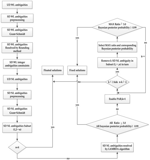
Figure 1.
A flowchart of partial ambiguity resolution of three-frequency UCPPP with predefined Bayesian posterior probability and ratio value.
2.3. Estimation, Representation, and Constraint of Atmospheric Corrections
To supply high-precision atmospheric corrections for users, the proper derivation and representation of atmospheric corrections play an essential role in the PPP-RTK performance. In this study, the PPP-RTK network component is mainly responsible for estimating atmospheric delays using a fixed ambiguity approach.
Combining Equation (7) with Figure 1, we can see that the accuracy of atmospheric delays can be ensured only when SD NL ambiguities can be resolved successfully. Therefore, the state vector of atmospheric delays can be estimated by constraining the fixed SD NL ambiguities. The specific forms are expressed as follows [45]:
where denotes the SD float NL ambiguity that can be accurately resolved; presents the fixed SD NL ambiguity; refers to the covariance matrix of UD float ambiguity; denotes the covariance matrix, considering the relationship between the remaining estimated parameters and the float UD ambiguity; represents the transformation matrix that maps from the UD float ambiguity and to the SD float ambiguity; and denote the vectors of the floating and fixed solutions, respectively; and represent the covariance matrices of the floating and fixed solutions, respectively.
After the atmospheric delays were derived from the reference sites, we applied the interpolation method to interpolate the atmospheric delays. Over the past few decades, many interpolated algorithms have been developed [46,47,48]. Because the interpolated errors mainly represent distance-dependent biases, the distance-based linear interpolation method (DIM) can be used to interpolate atmospheric delays [49]. Using the DIM approach, atmospheric corrections of satellite s visible to the user are interpolated from n reference stations and weighted by the inverse distance between the reference network and the user stations. The interpolated atmospheric corrections, including slant ionospheric and tropospheric delays, can be calculated as follows:
where refers to the distance between the user station and reference station i (km); denotes the interpolated slant ionospheric correction of satellite s visible to the user; denotes the pure slant ionospheric delay of satellite s visible to the reference station i and user components; represents the slant ionospheric delay contaminated by receiver DCBs from reference station i; is the receiver DCBs at reference station i; is the interpolated ZWD correction at user components; denotes the ZWD derived from reference station i; and indicates the number of reference stations.
The variance of interpolated atmospheric corrections is associated with two aspects of the stochastic model of atmospheric corrections. One is the uncertainty due to multiple path errors and observation noise. The other is the interpolated error, which mainly depends on the distance between the reference site and user location [49]. Normally, the variance of atmospheric corrections increases as the distance between the reference network and user increases. Thus, the variance of the atmospheric corrections can be calculated as follows:
where refers to the variance of interpolated slant ionospheric correction of satellite s; is the uncertainty of slant ionospheric delay of satellite s estimated from reference station i; denotes the variance of slant ionospheric delay of satellite s containing the effect of both the uncertainty of reference station i and interpolated errors from DIM; indicates the elevation angle of satellite s; mm/km is considered as the empirical scale factor of slant ionospheric delay [50,51,52]; is the variance of interpolated ZWD correction at user component; denotes the uncertainty of ZWD from reference station i; represents the variance of ZWD of reference station i containing the effect of both uncertainty of reference station i and interpolated errors from DIM; mm/km is considered as the empirical scale factor of zenith wet delay.
Figure 2 shows the geometric relationship between the location of the user and reference stations when utilizing the DIM method to interpolated atmospheric delays. The slant ionospheric correction of a given satellite (s) visible to the user can be interpolated by utilizing the slant ionospheric delays of the same satellite visible to the reference stations. When atmospheric corrections/variances are available for a certain epoch, the user can use them to enhance the PPP-RTK performance.
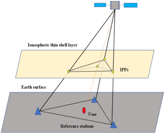
Figure 2.
DIM interpolation geometry.
For the user component, atmospheric correction can be used to enhance the PPP-RTK performance. The interpolated atmospheric correction retrieved from the reference network is considered as a pseudo-observation to accelerate the UCPPP ambiguity resolution. Specifically, the atmosphere-augmented UCPPP model of the user implementation is represented as follows:
where and denote the interpolated slant ionospheric correction and the corresponding variance calculated using Equations (18) and (19), respectively; is the difference between the interpolated slant ionospheric correction from the reference network component and the estimated slant ionospheric delay from the user component; and represent the interpolated zenith wet delay and corresponding variance, respectively; denotes the difference between the interpolated zenith wet delay from the reference network component and the estimated zenith wet delay from the user component.
Considering the above pseudo-observations of atmospheric augmentation, we can extend the three-frequency UCPPP function model in Equation (7) to compensate for variation in the estimated atmospheric delays in the PPP-RTK of the user components. Combining Equations (20) and (21), the UCPPP stochastic model can be represented as:
where and refer to the variance–covariance matrix of the raw pseudo-range and carrier phase measurements, respectively; denotes the variance–covariance matrix of slant ionospheric correction for the user components; denotes the variance–covariance matrix of zenith wet delay for the user components; and represents the identity matrix. The notation blkdiag refers to a block diagonal matrix.
3. Results
In this section, we first introduce the data selection and processing strategies for PPP-RTK of both the user and reference network components. Then, the performance of the UCPPP ambiguity resolution can be assessed by comparing the Gram–Schmidt method with the highest elevation angle method. Next, we assess the accuracy of atmospheric corrections by employing the difference between the estimated values from the user component and the interpolated values from the reference network. Furthermore, we also study the difference between atmospheric corrections using the Gram–Schmidt method and atmospheric corrections utilizing the highest elevation angle method. Finally, we investigated the positioning performance of PPP-RTK in the pseudo-kinematic mode.
3.1. Data Selection and Processing Strategies
To validate PPP-RTK performance, five stations were used in this study. These stations belong to the European reference frame (EUREF) Permanent GNSS Network (EPN), while those stations in Belgium, which are able to track multi-frequency observations. The observations condition of this reference network supplies a very good opportunity to assess PPP-RTK performance based on three-frequency observations. The station distributions are shown in Figure 3. In Figure 3, the reference stations marked by blue circles are used to estimate atmospheric corrections, whereas the red circle is considered as a user station to evaluate PPP-RTK performance. The average distance between the user positions and reference network varied from 30 to 100 km.
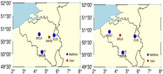
Figure 3.
Distribution of the reference network and user station. The blue circles refer to reference stations, and the red circle indicates the user station.
The station information for the five stations, including the station name, receiver type, and antenna type, is presented in Table 2.
Table 2.
Station information of five stations.
In this study, we adopted GPS observations on the day of the year (DOY) 082 and 083 in 2021. Table 3 summarizes the PPP-RTK data-processing strategies for both reference network and user components. The standard deviation of the zenith direction is 0.3 m and 0.3 cm for pseudo-range and carrier phase observations, respectively, which is regarded as an appropriate choice in most cases [53]. In addition, we used the Saastamoinen model [54] to correct tropospheric dry delays, and the global mapping function (GMF) [55] was considered as a mapping function to map slant dry and wet delays to zenith delays.
Table 3.
Processing strategies for PPP-RTK network and user component.
Figure 4 shows the number of satellites and position dilution of precision (PDOP) from the WARE and BRUX stations. The number of satellites varied from 7 to 13. The PDOP value ranged from two to four most of the time. Of course, there is an abnormal result of the PDOP between 12 and 14 h, and the number of satellites was relatively small at this time.
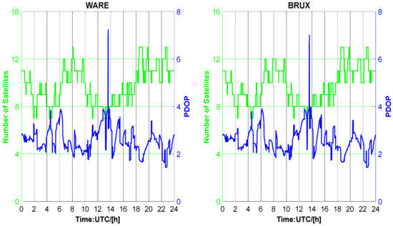
Figure 4.
Number of satellites and PDOP from WARE and BRUX station on DOY 082, 2021.
3.2. Performance of UCPPP Aambiguity Resolution
To assess the performance of UCPPP partial ambiguity resolution, we reinitialized every hour during the data processing of the PPP-RTK user component. We used three indicators to analyze the performance of the UCPPP PAR algorithm based on atmospheric augmentation. These indicators included the ratio test, epoch fixing rate, and TTFF. Four groups of UCPPP PAR solutions were prepared and compared: dual-frequency highest elevation angle solution (F2-MAX), dual-frequency Gram–Schmidt solution (F2-ALT), three-frequency highest elevation angle solution (F3-MAX), and three-frequency Gram–Schmidt solution (F3-ALT). Figure 5 shows four groups of UCPPP solutions.
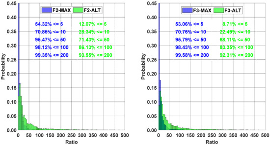
Figure 5.
Ratio distribution of UCPPP PAR.
It can be seen that the 54.32% of ratio distribution was under 5 for the F2-MAX, and 12.07% of the ratio distribution was under 5 for the F2-ALT. Similarly, when the range distribution was 50, the proportions of F2-MAX and F2-ALT were 95.47% and 71.43%, respectively. The right panel of Figure 5 also shows that the ratio distribution range of F3-ALT was larger than that of F3-MAX. Specifically, 95.79% of the ratio distribution proportions were under 50, whereas 68.11% of ratio distribution proportions fell within this range. A comparison of the distribution results of the ALT and MAX methods revealed that the ratio distribution range of the ALT method was larger than that of the MAX method. Meanwhile, the proportions of the ratio distribution of F2-ALT were slightly larger than those of F3-ALT within a certain distribution range.
Figure 6 shows the epoch fixing rate of the UCPPP PAR approach, which includes F2-MAX, F2-ALT, F3-MAX, and F3-ALT solutions. For DOY 082 in the WARE station, compared with the results of the MAX method, the epoch fixing rate of the ALT method was improved by 16.63% (from 79.20% to 95.83%) in dual-frequency UCPPP PAR and by 16.67% (from 81.87% to 98.54%) in three-frequency UCPPP PAR. Similar results occurred on the other three modes: BRUX-082, WARE-083, and BRUX-083. F2-MAX showed the smallest epoch fixing rate, excluding WARE-083, whereas F3-ALT showed the largest epoch fixing rate. Additionally, the epoch fixing rate of F3-ALT was higher than that of F2-ALT. An average improvement of 2.04% can be achieved. Furthermore, the average epoch fixing rates were 81.01, 95.92, 82.05, and 97.93% for F2-MAX, F2-ALT, F3-MAX, and F3-ALT, respectively. Overall, on the one hand, the average epoch fixing rate in F2-MAX is slightly lower than in F3-MAX, while the F2-ALT is slightly lower than in F3-ALT. In contrast, the average epoch fixing rate of F2-ALT was large than that of F2-MAX, while that of F3-ALT was larger than that of F3-MAX. This indicates that the ALT method has an advantage over the MAX method in terms of the epoch fixing rate. Moreover, the three-frequency methods also have certain advantages over the dual-frequency methods.
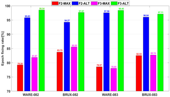
Figure 6.
Epoch fixing rate of UCPPP PAR.
Figure 7 shows the statistical results of the cumulative distribution of TTFF, which is considered the time taken to achieve ambiguity resolution. In F2-MAX, 75.60% of ambiguities can be resolved within 1 min, whereas this value is 80.45% for F2-ALT. Similarly, in three-frequency PAR, 78.04% of F3-MAX and 83.87% of F3-ALT can be fixed within 1 min. One can see that the ambiguity proportions of 89.02%, 94.25%, 90.24%, and 95.69% are within 3 min for F2-MAX, F2-ALT, F3-MAX, and F3-ALT, respectively. Furthermore, 91.46% of ambiguities can be resolved within 5 min for F2-MAX in contrast with 97.07% of ambiguities when F2-ALT was used for UCPPP PAR. In terms of three-frequency UCPPP PAR, an improvement of 3.99% can be achieved for F3-ALT compared to F3-MAX. It can be suggested that the ALT method has an obvious advantage over the MAX method regarding low TTFF. As the range of TTFF continued to increase, the difference between ALT and MAX decreased. Overall, the TTFF performance of F3-ALT was the best, whereas that of F2-MAX was slightly worse than those of the other three UCPPP PAR approaches.
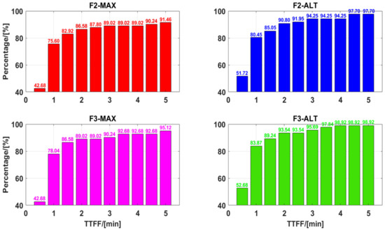
Figure 7.
Cumulative distribution of TTFF of UCPPP PAR.
3.3. Performance of Atmospheric Correction
In this section, the WARE and BRUX stations are considered as the reference stations for retrieving UD atmospheric corrections. The accuracy of atmospheric corrections was evaluated by differentiating the atmospheric delays estimated from the user components and interpolated from the reference network.
Figure 8 and Figure 9 show the error distribution of the zenith wet tropospheric corrections derived from the WARE and BRUX stations, respectively. It can be observed that most of the errors are within ±10 mm for the user stations. Furthermore, most of the errors were within ±5 mm for the WARE station. Meanwhile, the errors of zenith wet tropospheric corrections showed that the RMS of errors of 3 mm for the WARE station located in the reference network with an average distance of approximately 61 km, while the RMS of approximately 5 mm for the BRUX station was found at the reference network with an inter-station distance of approximately 81 km. Therefore, it was concluded that interpolated tropospheric corrections can be considered as accurate augmented information for improving UCPPP performance [56]. Unfortunately, compared with the highest elevation angle method, the Gram–Schmidt method does not exhibit an obvious advantage. In terms of the RMS of errors, the highest elevation angle method was slightly better than the Gram–Schmidt method. Overall, there is no clear difference between the Gram–Schmidt method and the highest elevation angle method in assessing the accuracy of zenith wet tropospheric corrections.
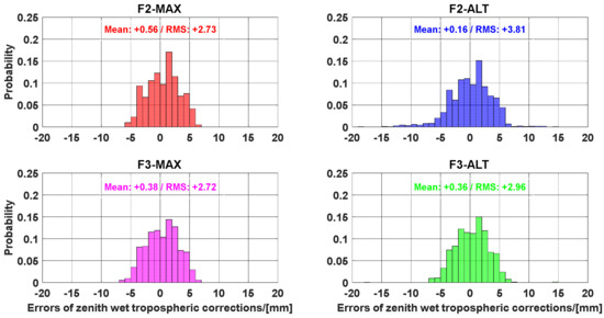
Figure 8.
Error distribution of the zenith wet tropospheric corrections from WARE station.
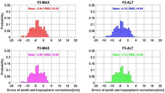
Figure 9.
Error distribution of the zenith wet tropospheric corrections from BRUX station.
Figure 10 and Figure 11 present the slant ionospheric delay variations estimated from the user stations and interpolated from the reference stations with the processing session. The negative values of the ionospheric delays were caused by the impact of the receiver’s DCBs, as shown in Equation (8). As can be seen, there is a clear systematic offset between the estimated slant ionospheric delays and interpolated slant ionospheric corrections. This systematic offset was more obvious at the BRUX station.
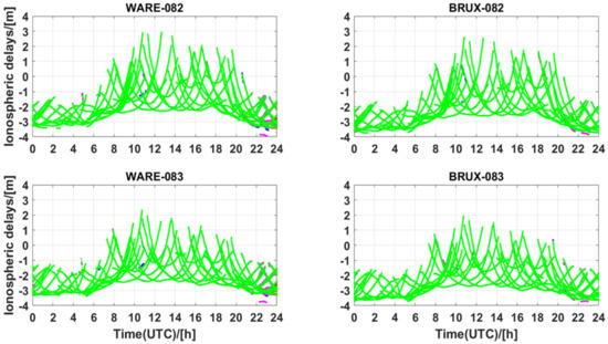
Figure 10.
Estimated slant ionospheric delays derived from WARE and BRUX stations on DOY 082, 083, 2021. The four groups of UCPPP PAR solutions—F2-MAX, F2-ALT, F3-MAX, and F3-ALT—are plotted as solid red, blue, pink, and green circles, respectively.
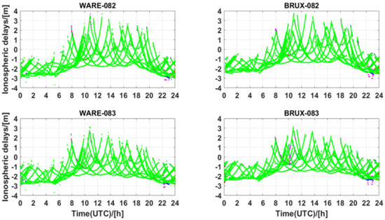
Figure 11.
Interpolated slant ionospheric delays of WARE and BRUX stations derived from the reference stations on DOY 082, 083, 2021. The four groups of UCPPP PAR solutions—F2-MAX, F2-ALT, F3-MAX, and F3-ALT֫—are plotted as solid red, blue, pink, and green circles, respectively.
Due to the color’s occlusion, we cannot precisely see the difference in slant ionospheric delays of the four methods; we roughly find that the ionospheric delays of F3-ALT are more continuous than those of the other three groups’ solutions, and there are few abnormal jumps in the processing sessions. Comparing the performance of UCPPP ambiguity fixing, it is not difficult to find that the results of slant ionospheric delays are related to the performance of ambiguity resolution. The different ambiguity fixing methods directly lead to different performances for slant ionospheric delays. Furthermore, a comparison of the results of the zenith wet tropospheric corrections reveals that the slant ionospheric delays are more closely related to the ambiguity parameters in the UCPPP model than the tropospheric delays.
The accuracy of the slant ionospheric delays interpolated from the reference stations and estimated from the user stations are shown in Figure 12 and Figure 13, respectively. Regardless of the interpolated accuracy or estimated accuracy, different AR approaches have little effect on their accuracy distribution. However, because the distance error affects the interpolated accuracy of the ionospheric delays, the interpolated accuracy of ionospheric delays is lower than that of the estimated ionospheric delays, as shown in Equation (19).
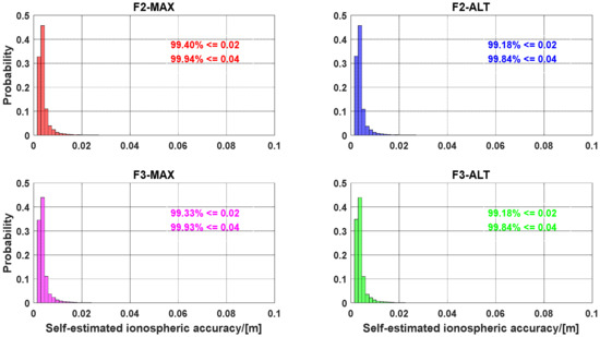
Figure 12.
Accuracy distribution of the estimated slant ionospheric delays derived from the user stations.
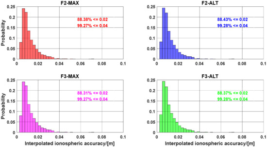
Figure 13.
Accuracy distribution of the interpolated slant ionospheric delays derived from the reference stations.
To further investigate the distribution characteristics of the difference between the estimated slant ionospheric delays and interpolated slant ionospheric delays, the results are shown in Figure 14. As expected, the F3-ALT solutions exhibited the best stability, except that there were some outliers owing to the hourly initialization. This is because the problem of ambiguity fixing causes anomalies in the slant ionospheric delays estimated from the reference network, which in turn causes jumps in SD slant ionospheric delays. Furthermore, slant ionospheric delays contaminated the receivers’ DCBs. This means that the SD ionospheric delays were affected by the difference between the weighted DCBs from the reference stations and the user DCBs (Xiang et al. 2020). Fortunately, the difference in receiver type is very small, which determines the difference between interpolated DCBs from the reference network and the estimated DCBs from the user stations. When the receiver types are the same or the difference is very small, the residuals of the receiver’s DCBs may be properly compensated for by estimating the residuals of the slant ionospheric delays. Therefore, fast and reliable ambiguity resolution can be achieved. Otherwise, the strength of the UCPPP model after atmospheric augmentation is affected, which in turn affects ambiguity fixing and positioning performance.
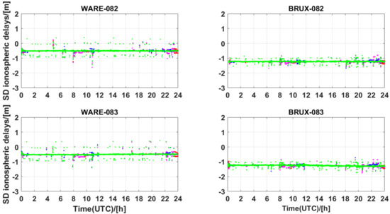
Figure 14.
SD slant ionospheric delays of WARE and BRUX stations; difference between the interpolated slant ionospheric corrections derived from the reference network and estimated slant ionospheric delays derived from the user stations on DOY 082, 083, 2021. The four groups of UCPPP PAR solutions—F2-MAX, F2-ALT, F3-MAX, and F3-ALT—are plotted as solid red, blue, pink, and green circles, respectively.
Figure 14 shows the characteristics of SD slant ionospheric delays. However, the impact of the receiver’s DCBs may be contained in SD ionospheric delays. To assess the accuracy of the slant ionospheric delays after eliminating the influence of the receiver’s DCBs, we performed the SD between satellites based on the original SD slant ionospheric delays. Based on the above analysis, the error distribution of the SD slant ionospheric delays is shown in Figure 15. For F2-MAX solutions, 91.32% of SD slant ionospheric residuals were within ±0.15 TECU, while 95.08% fell within ±0.25 TECU. The F2-ALT solutions within ±0.15 TECU account for 91.78% of SD ionospheric residuals, in contrast to 95.93% of SD ionospheric residuals being within ±0.25 TECU. From the bottom-right panel of Figure 15, it can be seen that 91.99% of the SD slant ionospheric residuals fall in ±0.15 TECU, which is worse than 93.45% for the F3-ALT method, which may imply an advantage over the F3-MAX method. Similarly, 95.68 and 96.98% of SD ionospheric residuals were within ±0.25 TECU in F3-MAX and F3-ALT, respectively. Overall, for both panels, regardless of whether dual-frequency or three-frequency conditions are used, the Gram–Schmidt method (ALT) always has a clear advantage over the highest elevation angle (MAX) approach. Combining the performance of UCPPP PAR, this fact suggests that the Gram–Schmidt strategy is reasonable for resolving SD NL ambiguities in contrast to the highest elevation angle approach.
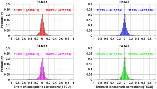
Figure 15.
Error distribution of the SD slant ionospheric corrections.
3.4. Performance of Kinematic PPP-RTK
In this section, the observations of the WARE and BRUX stations from DOY 082, 083, 2021 are utilized to assess the performance of PPP-RTK with the estimated unknowns reset to 1 h. Figure 16, Figure 17, Figure 18 and Figure 19 show a four-group solution comparison of UCPPP PAR with atmospheric augmentation in WARE-082, WARE-083, BRUX-082, and BRUX-083. During most of the processing sessions, 3D positioning errors can converge almost instantaneously. As expected, the F3-ALT solution showed better performance of convergence and positioning accuracy than the other three solutions, which is consistent with the assessment performance of both slant ionospheric delays and ambiguity resolution. We can also see that the performance of the three-frequency PPP-RTK has an obvious advantage over the dual-frequency PPP-RTK. Furthermore, it is noted that the time when the abnormal positioning results appear is highly consistent with the time when the abnormal accuracy of the ionospheric delays appears. Hence, determining which type of variance should be used to ensure a reasonable positioning accuracy becomes an essential problem and should be further researched in the future. In addition, the accuracy of the ionospheric corrections largely depends on the reliability of the corrected ambiguity fixing. An efficient and robust ambiguity resolution algorithm is crucial for both the PPP-RTK network and the user components.
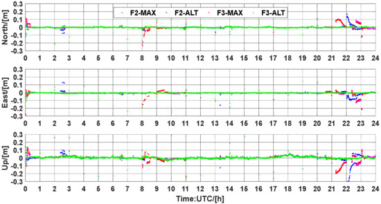
Figure 16.
Position errors for UCPPP PAR using the atmospheric corrections from WARE station on DOY 082, 2021.
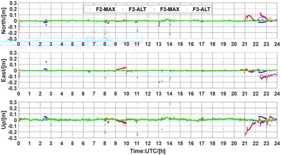
Figure 17.
Position errors for UCPPP PAR using the atmospheric corrections from WARE station on DOY 083, 2021.
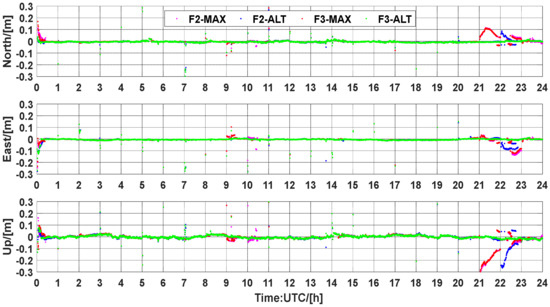
Figure 18.
Position errors for UCPPP PAR using the atmospheric corrections from BRUX station on DOY 082, 2021.
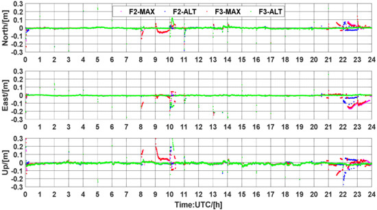
Figure 19.
Position errors for UCPPP PAR using the atmospheric corrections from BRUX station on DOY 083, 2021.
4. Discussion and Conclusions
In this study, we investigated the performance of GPS dual- and three-frequency PPP-RTK by comparing the Gram–Schmidt and highest elevation angle methods. For the assessment of ambiguity resolution, 95.47% and 71.43% of the ratio fell below 50 based on dual-frequency UCPPP AR for the highest elevation angle and Gram–Schmidt methods, respectively. In terms of epoch fixing rate, an average improvement of 2.04% was achieved, and the average epoch fixing rates were 81.01%, 95.92%, 82.05%, and 97.93% for F2-MAX, F2-ALT, F3-MAX, and F3-ALT, respectively. For TTFF, 75.60% of SD NL ambiguities in F2-MAX solutions can be fixed within 1 min, whereas that value is 80.45% for F2-ALT. Sequentially, 78.04% of F3-MAX and 83.87% of F3-ALT can be resolved within 1 min. Similarly, the SD NL ambiguity proportions of 89.02%, 94.25%, 90.24%, and 95.69% were within 3 min for F2-MAX, F2-ALT, F3-MAX, and F3-ALT, respectively.
As far as the accurate evaluation of the interpolated atmospheric corrections is concerned, most errors of the interpolated zenith wet tropospheric corrections are within ±10 mm. The zenith wet tropospheric corrections can be sufficiently accurate to augment PPP performance [56]. The statistical results of ionospheric delays demonstrated that 91.32% of SD ionospheric residuals were within 0.15 TECU in F2-MAX solution, in contrast to 95.08% being within 0.25 TECU. For the F2-ALT approach, 91.78% of SD ionospheric residuals derived are within 0.15 TECU, whereas 95.93% fall within 0.25 TECU for the F2-MAX solution. In three-frequency PPP-RTK, 91.99% and 93.45% of SD ionospheric residuals fall within 0.15 TECU for F3-MAX and F3-ALT, respectively. For the range of 0.25 TECU, 95.68% and 96.98% of SD ionospheric residuals can be achieved by the F3-MAX and F3-ALT methods, respectively. Finally, the positioning performance of PPP-RTK was assessed. Four groups of UCPPP PAR solutions can be assigned to the user’s positioning performance. As expected, the F3-ALT solution exhibited the best performance in terms of convergence and positioning accuracy. The other three approaches have inaccurate atmospheric information constraints at certain times, resulting in incorrect ambiguity fixing and large positioning error. Overall, the accuracy of interpolated ionospheric corrections largely depends on the reliability of the corrected ambiguity resolution. Hence, the ambiguity resolution algorithm plays an essential role in the PPP-RTK network and user components.
Although the expected results could be verified, our work only focused on the validation of the results by utilizing limited three-frequency GPS measurements from a two-PAR algorithm. Atmospheric delays have many complicated spatial and temporal characteristics. Therefore, it is essential to conduct an in-depth analysis of PPP-RTK performance in combination with the proposed PPP AR algorithm to investigate scenarios with different altitudes, latitudes, and high and low years of solar activity. Moreover, it is expected that the performance of PPP-RTK can be further improved by employing multi-frequency and multi-GNSS measurements. The advantages of multi-frequency and multi-GNSS PPP-RTK performance under different atmospheric conditions should be comprehensively investigated in the future.
Author Contributions
Conceptualization, Z.Y.; methodology, Z.Y.; software, Z.Y.; validation, X.Z.; investigation, Z.Y.; writing original draft preparation, Z.Y.; writing—review and editing, X.Z.; visualization, Z.Y.; supervision, X.Z. All authors have read and agreed to the published version of the manuscript.
Funding
This research was funded by the National Science Fund for Distinguished Yong Scholars (No. 41825009) and Changjiang Scholars Program.
Institutional Review Board Statement
Not applicable.
Informed Consent Statement
Not applicable.
Data Availability Statement
The precise orbit and clock products from GFZ and CNES are obtained at ftp://ftp.gfz-potsdam.de/pub/GNSS/products/mgex/, (accessed on 5 March 2022) and https://www.ppp-wizard.net/products/POST_PROCESSED/2021/082 (accessed on 5 March 2022); multi-GNSS observations are available through EUREF and NCN data centers (ftp://ftp.epncb.oma.be/pub/obs/2021/082 (accessed on 5 March 2022); https://geodesy.noaa.gov/corsdata/rinex/2021/082 (accessed on 5 March 2022)).
Acknowledgments
The GFZ, CNES Analysis Center, EUREF Permanent GNSS Network and National Geodetic survey are appreciated for providing access to multi-GNSS products and multi-GNSS observations.
Conflicts of Interest
The authors declare no conflict of interest.
References
- Zumberge, J.; Heflin, M.; Jefferson, D.; Watkins, M.; Webb, F. Precise point positioning for the efficient and robust analysis of GPS data from large networks. J. Geophys. Res. 1997, 102, 5005–5017. [Google Scholar] [CrossRef] [Green Version]
- Kouba, J.; Heroux, P. Precise Point Positioning Using IGS Orbit and Clock Products. GPS Solut. 2011, 5, 12–28. [Google Scholar] [CrossRef]
- Ge, M.; Gendt, G.; Rothacher, M.; Shi, C.; Liu, J. Resolution of GPS carrier-phase ambiguities in Precise Point Positioning (PPP) with daily observations. J. Geod. 2008, 82, 389–399. [Google Scholar] [CrossRef]
- Collins, P. Isolating and estimating undifferenced GPS integer ambiguities. In Proceedings of the ION NTM, San Diego, CA, USA, 28–30 January 2008; pp. 720–732. [Google Scholar]
- Laurichesse, D.; Mercier, F.; Berthias, J.P.; Broca, P.; Cerri, L. Integer ambiguity resolution on undifferenced GPS phase measurements and its application to PPP and satellite precise orbit determination. Navigation 2009, 56, 135–149. [Google Scholar] [CrossRef]
- Bertiger, W.; Desai, S.D.; Haines, B.; Harvey, N.; Moore, A.W.; Owen, S.; Weiss, J.P. Single receiver phase ambiguity resolution with GPS data. J. Geod. 2010, 84, 327–337. [Google Scholar] [CrossRef]
- Teunissen, P.J.G.; Odijk, D.; Zhang, B. PPP-RTK: Results of CORS network-based PPP with integer ambiguity resolution. J. Aeronaut. Astronaut. Aviat. 2010, 42, 223–229. [Google Scholar]
- Geng, J.; Meng, X.; Dodson, R.; Teferle, F.N. Integer ambiguity resolution in precise point positioning: Method comparsion. J. Geod. 2010, 84, 569–581. [Google Scholar] [CrossRef] [Green Version]
- Shi, J.; Gao, Y. A comparison of three PPP integer ambiguity resolution methods. GPS Solut. 2014, 18, 519–528. [Google Scholar] [CrossRef]
- Teunissen, P.J.G.; Khodabandeh, A. Review and principles of PPP-RTK methods. J. Geod. 2015, 89, 217–240. [Google Scholar] [CrossRef]
- Wubbena, G.; Schimitz, M.; Bagge, A. PPP-RTK: Precise Point Positioning Using Sate-Space Representation in RTK Networks. In Proceedings of the 18th International Technical Meeting of the Satellite Division, Long Beach, CA, USA, 13–16 September 2005; pp. 2584–2594. [Google Scholar]
- Li, X.; Zhang, X.; Ge, M. Regional reference network augmented precise point positioning for instantaneous ambiguity resolution. J. Geod. 2011, 85, 151–158. [Google Scholar] [CrossRef]
- Nadarajah, N.; Khodabandeh, A.; Wang, K.; Choudhury, M.; Teunissen, P.J.G. Multi-GNSS PPP-RTK: From Large- to Small-Scale Networks. Sensors 2018, 18, 1078. [Google Scholar] [CrossRef] [PubMed] [Green Version]
- Li, Z.; Chen, W.; Ruan, R.; Liu, X. Evaluation of PPP-RTK based on BDS-3/BDS-2/GPS observations: A case study in Europe. GPS Solut. 2020, 24, 38. [Google Scholar] [CrossRef]
- Psychas, D.; Verhagen, S. Real-Time PPP-RTK Performance Analysis Using Ionospheric Corrections from Multi-Scale Network Configurations. Sensors 2020, 20, 3012. [Google Scholar] [CrossRef] [PubMed]
- Zha, J.; Zhang, B.; Liu, T.; Hou, P. Ionosphere-weighted undifferenced and uncombined PPP-RTK: Throretical models and experimental results. GPS Solut. 2021, 25, 135. [Google Scholar] [CrossRef]
- Gao, W.; Zhao, Q.; Meng, X.; Pan, S. Performance of Single-Epoch EWL/WL/NL Ambiguity-Fixed Precise Point Positioning with Regional Atmosphere Modelling. Remote Sens. 2021, 13, 3758. [Google Scholar] [CrossRef]
- Zhang, X.; Ren, X.; Chen, J.; Zuo, X.; Mei, D.; Liu, W. Investigating GNSS PPP-RTK with external ionospheric constraints. Satell. Navig. 2022, 3, 6. [Google Scholar] [CrossRef]
- Li, X.; Wang, B.; Li, X.; Huang, J.; Lyu, H.; Han, X. Principle and performance of multi-frequency and multi-GNSS PPP-RTK. Satell. Navig. 2022, 3, 7. [Google Scholar] [CrossRef]
- Zhang, B.; Hou, P.; Zha, J.; Liu, T. PPP-RTK functional models formulated with undifferenced and uncombined GNSS observations. Satell. Navig. 2022, 3, 3. [Google Scholar] [CrossRef]
- Keshin, M.; Sato, Y.; Nakakuki, K.; Hirokawa, R. A Novel Clock Parameterization and Its Implications for Precise Point Positioning and Ionosphere Estimation. Sensors 2022, 22, 3117. [Google Scholar] [CrossRef]
- Teunissen, P.J.G.; Verhagen, S. GNSS carrier phase ambiguity resolution: Challenges and open problems. In Observing Our Changing Earth; Sideris, M.G., Ed.; Springer: Berlin, Germany, 2009; pp. 785–792. [Google Scholar]
- Verhagen, S.; Teunissen PJ, G.; van der Marel, H.; Li, B. GNSS ambiguity resolution: Which subset to fix. In Proceedings of the IGNSS Symposium, Sydney, Australia, 15–17 November 2011; pp. 15–17. [Google Scholar]
- Wang, J.; Feng, Y. Reliability of partial ambiguity fixing with multiple GNSS constellations. J. Geod. 2013, 87, 1–14. [Google Scholar] [CrossRef]
- Li, P.; Zhang, X. Precise Point Positioning with Partial Ambiguity Fixing. Sensors 2015, 15, 13627–13643. [Google Scholar] [CrossRef] [PubMed] [Green Version]
- Pan, Z.; Cai, H.; Liu, J.; Dong, B.; Liu, M.; Wang, H. GPS partial ambiguity resolution method for zero-difference precise point positioning. Acta Geod. Cartogr. Sin. 2015, 44, 1210–1218. [Google Scholar]
- Wu, J.T.; Wu, S.C.; Hajj, G.A.; Bertiger, W.I.; Lichten, S.M. Effects of antenna orientation on GPS carrier phase. Manuscr. Geod. 1993, 18, 91–98. [Google Scholar]
- Xu, G.; Xu, Y. GPS: Theory, Algorithms and Applications; Springer: Berlin, Germany, 2016. [Google Scholar]
- Petit, G.; Luzum, B. IERS Technical Note No.36, IERS Conventions 2010; International Earth Rotation and Reference Systems Service: Frankfurt, Germany, 2010. [Google Scholar]
- Liu, T.; Chen, H.; Chen, Q.; Jiang, W.; Laurichesse, D.; An, X.; Geng, T. Characteristics of phase bias from CNES and its application in multi-frequency and multi-GNSS precise point positioning with ambiguity resolution. GPS Solut. 2021, 25, 25–58. [Google Scholar] [CrossRef]
- Guo, F.; Zhang, X.; Wang, J. Timing group delay and differential code bias corrections for BeiDou positioning. J. Geod. 2015, 89, 427–445. [Google Scholar] [CrossRef]
- Guo, F.; Zhang, X.; Wang, J.; Ren, X. Modeling and assessment of triple-frequency BDS precise point positioning. J. Geod. 2016, 90, 1223–1235. [Google Scholar] [CrossRef]
- Laurichesse, D.; Privat, A. An Open-source PPP Client Implementation for the CNES PPP-WIZARD Demonstrator. In Proceedings of the ION GNSS+ 2015, Tampa, FL, USA, 14–18 September 2015. [Google Scholar]
- Naciri, N.; Bisnath, S. An uncombined triple-frequency user implementation of the decoupled clock model for PPP-AR. J. Geod. 2021, 95, 60. [Google Scholar] [CrossRef]
- Geng, J.; Teferle, F.N.; Meng, X.; Dodson, A.H. Towards PPP-RTK: Ambiguity resolution in real-time precise point positioning. Adv. Space Res. 2011, 47, 1664–1673. [Google Scholar] [CrossRef] [Green Version]
- Li, P.; Zhang, X.; Ren, X.; Zuo, X.; Pan, Y. Generating GPS satellite fractional cycle bias for ambiguity-fixed precise point positioning. GPS Solut. 2016, 20, 771–782. [Google Scholar] [CrossRef]
- Li, P.; Zhang, X.; Guo, F. Ambiguity resolved precise point positioning with GPS and BeiDou. J. Geod. 2017, 91, 25–40. [Google Scholar]
- Teunissen, P.J.G. The least-squares ambiguity decorrelation adjustment: A method for fast GPS integer ambiguity estimation. J. Geod. 1995, 70, 65–82. [Google Scholar] [CrossRef]
- Dong, D.; Bock, Y. Global positioning system network analysis with phase ambiguity resolution applied to crustal deformation studies in California. J. Geophys. Res. 1989, 94, 3949–3966. [Google Scholar] [CrossRef]
- Ge, M.; Gendt, G.; Dick, G.; Zhang, F.P. Improving carrier-phase ambiguity resolution in global GPS network solutions. J. Geod. 2005, 79, 103–110. [Google Scholar] [CrossRef]
- Ren, K.; Song, X.; Jia, X. Using Orthogonal Transformation Method to Select Independent Baselines and Independent Double-difference Ambiguities. Acta Geod. Cartogr. Sin. 2016, 41, 974–977. [Google Scholar]
- Teunissen, P.J.G. Success probability of integer GPS ambiguity rounding and bootstrapping. J. Geod. 1998, 72, 606–612. [Google Scholar] [CrossRef] [Green Version]
- Wu, Z.; Bian, S. GNSS integer ambiguity validation based on posterior probability. J. Geod. 2015, 89, 961–977. [Google Scholar] [CrossRef]
- Euler, H.J.; Schaffrin, B. On a measure of the discernibility between different ambiguity solutions in the static-kinematic GPS mode. In Kinematic Systems in Geodesy, Surveying and Remote Sensing; Schwarz, K.P., Lachapelle, G., Eds.; Springer: New York, NY, USA, 1990; pp. 285–295. [Google Scholar]
- Li, B.; Shen, Y.; Feng, Y.; Gao, W.; Yang, L. GNSS ambiguity resolution with controllable failure rate for long baseline network RTK. J. Geod. 2014, 88, 99–112. [Google Scholar] [CrossRef]
- Wanninger, L. Improved AR by regional differential modeling of the ionosphere. In Proceedings of the 8th International Technical Meeting of the Satellite Division of the US Institute of Navigation, Palm Springs, CA, USA, 12–15 September 1995; pp. 55–62. [Google Scholar]
- Han, S. Carrier Phase-Based Long-Range GPS Kinematic Positioning. Ph.D. Thesis, The University of New South Wales, Sydney, Australia, 1997. [Google Scholar]
- Gao, Y.; Li, Z.; McLellan, J. Carrier phase based regional area differential GPS for decimeter-level positioning and navigation. In Proceedings of the 10th International Technical Meeting of the Satellite Division of US Institute of Navigation, Kansas, MO, USA, 16–19 September 1997; pp. 1305–1313. [Google Scholar]
- Xiang, Y.; Gao, Y.; Li, Y. Reducing convergence time of precise point positioning with ionospheric constraints and receiver differential code bias modeling. J. Geod. 2020, 94, 8. [Google Scholar] [CrossRef]
- Odijk, D. Weighting ionospheric corrections to improve fast GPS positioning over medium distances. In Proceedings of the ION GNSS 2000, Institute of Navigation, Alexandria, VA, USA, 19–22 September 2000; pp. 1113–1123. [Google Scholar]
- Liu, G.; Lachapelle, G. Ionosphere weighted GPS cycle ambiguity resolution. In Proceedings of the ION National Technical Meeting, San Diego, CA, USA, 28–30 January 2002; pp. 1–5. [Google Scholar]
- Li, B.; Verhagen, S.; Teunissen, P.J.G. Robustness of GNSS integer ambiguity resolution in the presence of atmospheric biases. GPS Solut. 2014, 18, 283–296. [Google Scholar] [CrossRef]
- Li, B.; Shen, Y.; Xu, P. Assessment of stochastic models for GPS measurements with different types of receivers. Chin. Sci. Bull. 2008, 53, 3219–3225. [Google Scholar] [CrossRef] [Green Version]
- Saastamoinen, J. Atmospheric correction for the troposphere and stratosphere in radio ranging of satellites. In The Use of Artificial Satellites for Geodesy; Henriksen, S.W., Mancini, A., Chovitz, B.H., Eds.; Geophysical Monograph Series; AGU: Washington, DC, USA, 1972; Volume 15, pp. 247–251. [Google Scholar]
- Boehm, J.; Niell, A.; Tregoning, P.; Schuh, H. Global mapping function (GMF): A new empirical mapping function based on numerical weather model data. Geophys. Res. Lett. 2006, 33, L7304. [Google Scholar] [CrossRef] [Green Version]
- Zhou, P.; Wang, J.; Nie, Z.; Gao, Y. Estimation and representation of regional atmospheric corrections for augmenting real-time single-frequency PPP. GPS Solut. 2020, 24, 7. [Google Scholar] [CrossRef]
Publisher’s Note: MDPI stays neutral with regard to jurisdictional claims in published maps and institutional affiliations. |
© 2022 by the authors. Licensee MDPI, Basel, Switzerland. This article is an open access article distributed under the terms and conditions of the Creative Commons Attribution (CC BY) license (https://creativecommons.org/licenses/by/4.0/).