Fine-Grained Individual Air Quality Index (IAQI) Prediction Based on Spatial-Temporal Causal Convolution Network: A Case Study of Shanghai

Abstract

Accurate and fine-grained individual air quality index (IAQI) prediction is the basis of air quality index (AQI), which is of great significance for air quality control and human health. Traditional approaches, such as time series, recurrent neural network or graph convolutional network, cannot effectively integrate spatial-temporal and meteorological factors and manage the dynamic edge relationship among scattered monitoring stations. In this paper, a ST-CCN-IAQI model is proposed based on spatial-temporal causal convolution networks. Both the spatial effects of multi-source air pollutants and meteorological factors were considered via spatial attention mechanism. Time-dependent features in the causal convolution network were extracted by stacked dilated convolution and time attention. All the hyper-parameters in ST-CCN-IAQI were tuned by Bayesian optimization. Shanghai air monitoring station data were employed with a series of baselines (AR, MA, ARMA, ANN, SVR, GRU, LSTM and ST-GCN). Final results showed that: (1) For a single station, the RMSE and MAE values of ST-CCN-IAQI were 9.873 and 7.469, decreasing by 24.95% and 16.87% on average, respectively. R² was 0.917, with an average 5.69% improvement; (2) For all nine stations, the mean RMSE and MAE of ST-CCN-IAQI were 9.849 and 7.527, respectively, and the R² value was 0.906. (3) Shapley analysis showed PM₁₀, humidity and NO₂ were the most influencing factors in ST-CCN-IAQI. The Friedman test, under different resampling, further confirmed the advantage of ST-CCN-IAQI. The ST-CCN-IAQI provides a promising direction for fine-grained IAQI prediction.

1. Introduction

In recent years, under the background of rapid development of industrialization and urbanization in China, human factors have had a significant impact on urban air environment, which has directly led to different degrees of urban air pollution [1,2]. Among them, heavy air pollution poses a continuing threat to city dwellers. Long-term exposure to high concentrations of air pollution will significantly increase the risk of disease, causing serious damage to the human respiratory, nervous, cardiovascular and reproductive systems [3]. According to statistics, there are about one million deaths caused by air pollutants in China every year [4]. In addition, air pollution has been the main cause of death in the United States for nearly 25 years [5]. An accurate, effective and stable air quality index (AQI) prediction model is necessary, to promote urban public health and the sustainable development of society [6]. As the basis of AQI estimation, individual air quality index (IAQI) provides technical regulation from a single pollutant concentration (PM_2.5, PM₁₀, NO₂, etc.) perspective. The modeling of fine-grained IAQI forecasting can be regarded as a traditional time series prediction problem, and attracts massive attention from researchers and policymakers [6,7].

In order to get a sound IAQI prediction result, a successful or ‘ideal’ model should satisfy the following three conditions, as we summarize from the recent 10 years of literature:

Multiple impact factors should be considered as far as possible according to the actual monitoring station’s condition. These factors include meteorological factors (temperature, wind speed, precipitation, etc.), different pollutants, traffic distributions and so on. The interaction between pollutants should also be taken into account to improve the accuracy of prediction.

Since IAQI data are interdependent in spatial and temporal dimensions and usually have high autocorrelation, spatial-temporal dependencies among monitoring stations should be captured.

To make full use of the monitoring station’s information and get a better AQI estimation, the IAQI prediction model should be effective and robust for different individual air pollution concentrations (PM_2.5, PM₁₀, SO₃, NO₂, etc.).

Most of the current pioneering works mainly focus on modeling the spatial-temporal distribution characteristics of air quality data in the dynamic nonlinear system by data-driven means. The key to IAQI modeling is to extract time dependence and spatial correlation from data. Current methods for extracting time-dependent features (especially features over a long time span) include recurrent neural network (RNN) [8,9], gate recurrent unit (GRU) [10,11,12] and long–short term memory (LSTM) [13,14,15,16,17]. However, these RNN-based sequential approaches suffer from time-consuming iterative propagation, gradient explosion and vanishing problems [18]. The spatial correlation extraction among air pollutants is also considered in IAQI modeling via graph-based models and convolutional neural networks [19,20,21]. These methods inherit the First law of Geography (https://doi.org/10.2307/143141), and take the correlations among adjacent stations into consideration. Graph modeling has proven to improve accuracy because spatial dependency can be naturally expressed by graph node and edge weight in between [19]. Existing graph models tend to rely on Markovian assumptions to make modeling the interactions across variables tractable, assuming that a node’s future information is conditioned on its historical information as well as its neighbors’ historical information [20]. However, there are circumstances when a connection does not entail the interdependency relationship between two nodes, let alone the connection missing problem between graph nodes. Convolutional neural network (CNN)-based models enjoy the advantages of parallel computing and stable gradients [20,21], which can capture the spatial information of the local receptive field through the convolution kernel, and obtain the global spatial features through multilayer convolution and pooling. CNN-based models pave a new direction for accurate and fine-grained prediction of IAQI.

In view of the drawbacks in current studies, this paper proposes a fine-grained IAQI prediction model (ST-CCN-IAQI) based on spatial-temporal causal convolution network by integrating spatial-temporal characteristics and atmospheric environmental factors. Causal convolutional networks use stacked dilated convolution, which can effectively capture the time dependence between long distance time series. The receptive field size of stacked dilated casual convolution networks grows exponentially with an increase in the number of hidden layers. Convolutional neural network and spatial attention are combined to extract spatial information. The main contributions of this paper are as follows:

• In order to capture the nonlinear influencing factors, this paper considered the spatial-temporal correlation between stations, meteorological factors, and the interaction between different pollutants when modeling IAQI prediction.
• In this paper, the subtle differences between different types of deep learning were noted, and the causal convolutional network based on CNN was rewritten to extract spatial-temporal features using attention mechanism and stacked dilated convolution.
• The ST-CCN-IAQI proposed in this paper has been proved to be superior to the baseline models through cross-validation and Friedman test, which establishes a new baseline for IAQI prediction. This paper also analyzes the importance of each influencing factor to model prediction, which provides convenience for further modeling.

The rest of this paper is organized as follows: the second part discusses the current progress; the third part explains ST-CCN-IAQI in detail; the fourth part brings in the experiments; the fifth part fulfills discussion, and the sixth part summarizes the conclusions.

2. Related Works

2.1. On Modeling of Fine-Grained IAQI Prediction

2.1.1. Traditional Approaches

Traditional models amenable to fine-grained AQI prediction refer to specialized meteorological models, time series models, and shallow neural networks. The research on the meteorological model [22,23] is mainly based on the knowledge of pollutant formation and diffusion, and uses the prior knowledge of atmospheric physical and chemical processes as the basic theory of mass concentration prediction, so as to realize the simulation and prediction of the atmospheric pollutant concentration evolution process. The advantage of this deterministic method is that it has a solid theoretical basis and a relatively transparent model. With the deepening of the research on the physical and chemical process of air pollutants, the prediction performance of the model is improved. However, these deterministic methods rely heavily on theoretical assumptions and may lack key knowledge of physical processes, which makes it difficult to explain the nonlinearity and heterogeneity of many influencing factors, leading to AQI prediction bias [24]. Time series models (such as autoregressive (AR) model, moving average (MA) model and autoregressive moving average (ARMA) model) are the first choice to deal with IAQI sequences [25,26]. Barthwal utilized ARMA and autoregressive integrated moving average (ARIMA) time series models to predict the daily average AQI of Delhi National Capital District, India, and achieved good performance [25]. However, the diffusion evolution of air pollutants is a dynamic nonlinear process, and linear statistics and time series cannot reflect its complexity, and the prediction deviation is generally large.

Shallow neural networks, such as support vector regression (SVR) [27,28] and artificial neural network (ANN) [29,30] have been applied to sequential prediction tasks. Motesaddi et al. used ANN to study the AQI prediction of SO₂. This model can learn the complex nonlinear dependence between input and output well, and has good robustness and adaptive characteristics, which improves the prediction accuracy and has low time complexity [31]. Compared with time series models, shallow neural networks generally have better performance [31,32,33]. However, they are mostly limited to practical applications, since it is difficult to capture complex spatial-temporal dependency among stations and predict overall IAQI situations in a large-scale network [21,24].

2.1.2. Deep Learning-Based Models

In recent years, deep learning models have been widely used in air pollutant prediction. Currently, deep learning models are used for atmospheric pollutant concentration prediction and can be roughly divided into three categories: sequence-based, graph-based, and convolution-based.

Sequence-based models, such as RNN, LSTM, and GRU, have shown a considerable advantage in air pollutant prediction [25,34,35]. General sequence-based models take advantage of shared parameters and pass implicit states to extract the temporal dependency of the context. However, these sequential methods, based on RNN, have the problems of long iterative propagation time, gradient explosion and disappearance [18].

Graph-based models behave competitively in sequential modeling. The graph convolution generalizes the traditional convolution to data of graph structures [19]. Although the inclusion of graph modeling has proven to improve accuracy of prediction, current models have several serious limitations, such as the complexity of model training, the artificial definition of relationships between variables, and the use of Markov assumptions to define interactions between variables [20]. In our experiments, we have found it difficult to capture the stable edge relationship between dynamic time series with graph-based methods, due to various external influences.

Convolution-based models, such as causal convolution network (CCN) from the field of image processing have also been widely applied in time series prediction [24,25]. Convolution in the CCN architecture is causal, meaning that there is no information “leaking” into the past. Its back propagation path depends on the network depth, which avoids the time-consuming problem of iterative propagation of traditional RNN models. Therefore, CCN is simpler while more effective in sequential modeling [20,21]. In addition, CCN can obtain a flexible and adjustable receptive field by changing the network layer number, convolution kernel, inflation factor and other parameters [24].

2.2. On Selection of Impact Factors

2.2.1. Spatial-Temporal Influence Factors

The spatial-temporal correlation between the target station and adjacent stations has been used in IAQI prediction modeling. Jiao et al. took the prediction stations as the center and selected the data of the five nearest stations as the spatial information input [36]. Li et al. regarded administrative division as the spatial scope of surrounding stations [13]. Feng et al. obtained the pollution input path of the study area through air mass trajectory analysis, and artificially selected a station from each path as the spatial information input [37]. Pak et al. predicted IAQI by extracting the temporal and spatial correlation of time series of multiple monitoring stations at different locations, enabling the model to obtain more accurate and stable prediction performance [38]. However, current research methods still lack targeted optimization for spatial-temporal dependent feature extraction.

2.2.2. Other Influencing Factors

The interaction between air pollutants cannot be ignored in fine-grained IAQI modeling [39]. Zhang et al. point out that there is a strong correlation between PM_2.5 and other air pollutants [40]. In addition, meteorological factors, such as wind speed, humidity and so on, also play a significant role [24,40]. For example, wind direction, wind speed and other factors contribute to the diffusion in the air, while low atmospheric pressure will make air pollutants float and accumulate in the air [38].

It is concluded that air pollutants and meteorological factors should be considered comprehensively in the fine-grained IAQI prediction task to further improve the prediction performance of the model.

3. Methodology

The ST-CCN-IAQI proposed in this paper is based on the extraction of spatial-temporal autocorrelation from air quality data. Temporal autocorrelation means that values at one point in a time series depend on values at some point in the past. This paper takes this factor into consideration and employed stacked dilated convolution with temporal attention to extract temporal autocorrelation. The time attention module focused on the time intervals that were strongly correlated with each moment, and stacked dilated convolution could efficiently extract the time autocorrelation. In addition, we noted the potential interdependence (spatial autocorrelation) between observations in the adjacent region. Therefore, this paper not only resorted to Spearman rank correlation analysis to extract spatial autocorrelation between stations, but also alluded to the convolution neural network, based on spatial attention, to further optimize the spatial autocorrelation features, which served as the input of the end-to-end time feature extraction module. ST-CCN-IAQI introduced spatial-temporal autocorrelation into modeling and further optimized it by attention mechanism, which provided a feasible means for IAQI prediction.

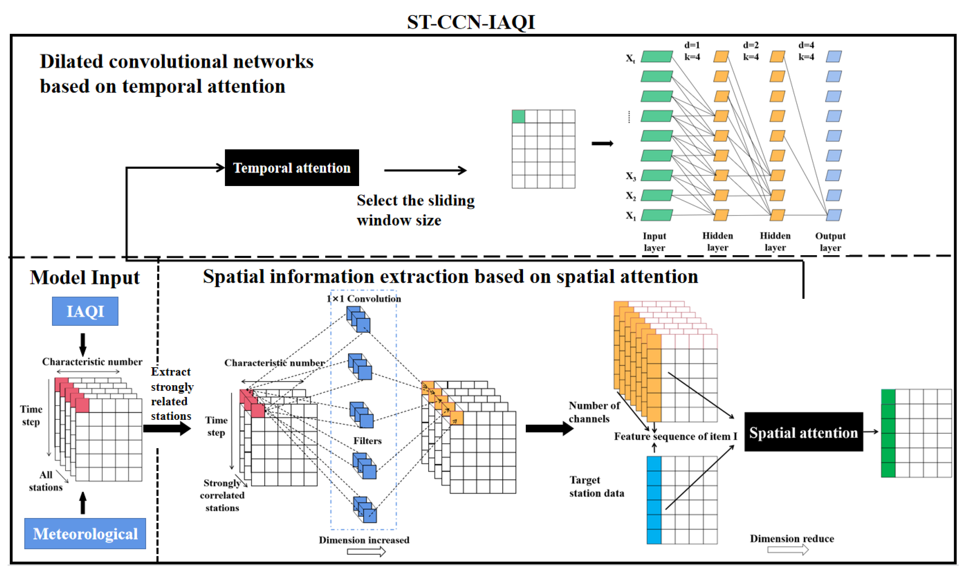
The ST-CCN-IAQI architecture is shown in Figure 1, which mainly consists of two parts: spatial feature extraction, based on convolutional neural network and spatial attention, and temporal feature extraction, based on temporal attention and stacked dilated convolution.

In this paper, the three-dimensional characteristic matrix $X\in R^{N\times T\times L}$ composed of air pollutant IAQI and meteorological data of multiple monitoring stations was used as the initial input, where $N$ represents all $N$ stations, $T$ represents the time step of historical data, and $L$ represents the characteristic dimension. In the module of spatial feature extraction, we used Spearman correlation analysis, convolutional neural network and spatial attention mechanism to extract spatial features that contributed greatly to the prediction of target stations as the input of the next stage. In the time feature extraction module, the time-attention mechanism was used to select highly interdependent time intervals as the input of stacked dilated convolutional network. Stacked dilated convolution extracts time-dependent features from the spatial feature matrix to predict IAQI.

3.1. Spatial Features Extraction

Spearman rank correlation coefficient was used to measure the degree of correlation between the historical sequence of surrounding stations and the historical sequence of the target station (the IAQI sequence that we were going to predict), and the correlation coefficient was between 0 and 1. The closer the correlation coefficient was to 1, the stronger the correlation between the two stations was. The calculation formula is as follows:

$${\rho (Y,Y}_k)=1-\frac{6{\sum }_{i=1}^N{(Y}^i{-Y}_k^i)}{{N(N}^2-1)}$$

(1)

In Formula (1) ${\rho (Y,Y}_k)$ represents the spearman correlation coefficient of the two sequences, where $Y$ represents the IAQI historical data sequence of the target station sorted in numerical descending order, $Y_k$ represents the sequence of IAQI historical data of a surrounding station sorted in numerical descending order, and N represents the number of samples in the sequence. For example, $\rho \_\mathit{list}$ in Formula (2) is the correlation coefficient we calculated between the target station and all stations.

$${\rho \_list=\left[\rho \right(Y}^{*}{,Y}_1{),\rho (Y}^{*}{,Y}_2),\dots {, \rho (Y}^{*}{,Y}_S\left)\right]$$

(2)

We compared the correlation coefficient with the threshold ${\rho }_{th}$, and finally obtained the set of $M$ stations with the correlation coefficient greater than ${\rho }_{th}$ as follows:

$${X=\{X}_i{\left|\rho \right(Y}^{*}{,Y}_i{)>\rho }_{th}, i\in 1,\dots ,M\}x$$

(3)

In Formula (3), $X_i\in R^{T\times L}$ is the feature matrix of the i-th station with strong spatial correlation with the target station, $X\in R^{M\times T\times L}$ represents the three-dimensional feature matrix with strong spatial correlation with the target station, where $M \le S$, $M$ represents the number of stations with strong spatial correlation with the target station, $T$ represents the time step of historical data, and $L$ represents feature dimension.

We used $1\times 1$ convolution kernel to realize the dimension raising of the feature matrix. After the dimension raising process, the three-dimensional matrix became $X\in R^{M_{new}\times T\times L}$, where $M_{new}$ represents the number of channels after dimension raising.

As shown in Figure 2, the $1\times 1$ convolution kernel in the convolutional neural network was used to raise the dimension of the feature matrix $A$ by increasing the number of output channels. The rectangular box in the middle contains $M_{new}$ filters, and the dimension of the filter was $1\times 1\times k$ ($k$ is the number of convolution kernels), where the number of convolution kernels is the same as the number of channels of the eigenmatrix. In the local perspective, the three red blocks are convolved with the $M_{new}$ filter to obtain $M_{new}$ orange blocks. From the global perspective, the number of channels of the original feature matrix was expanded, and the newly generated feature matrix was $X\in R^{M_{new}\times T\times L}$. In the process of dimension raising, the convolution operation of eigenmatrix and filter made the information from different channels interact and fuse, which improved the ability of nonlinear feature extraction of the model.

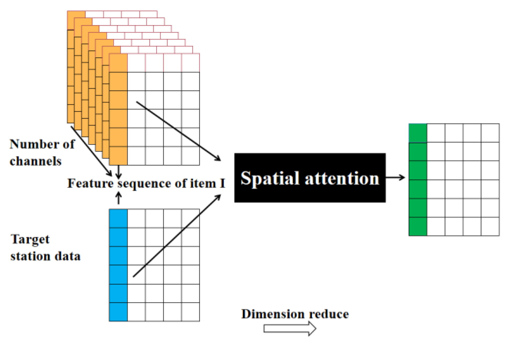
The following dimension reduction process of eigen matrix is based on spatial attention mechanism, as shown in Figure 3.

Firstly, the correlation coefficient between the i-th feature sequence of each channel and the i-th feature sequence of the target station was extracted, as shown in Formula (4). In Formula (4), ${\mathit{Sim}}_m^i$ represents the correlation coefficient between the feature sequence of the i-th item of the m-th channel and the target sequence.

$${\mathit{Sim}}_m^i{=\mathit{Similarity}(f}_{\mathit{target}}^i{,f}_m^i{)=\mathit{Spearman}(f}_{\mathit{target}}^i{,f}_m^i)$$

(4)

Then the weight distribution of the i-th item sequence of each channel was calculated based on the correlation coefficient. SoftMax was used to carry out numerical conversion of the correlation coefficients, and the original correlation coefficients were transformed into probability distribution with the sum of the weights of all elements being 1, so that the weight of important feature sequences could be highlighted. The calculation is as follows:

$$a_m^i{=\mathit{Softmax}(\mathit{Sim}}_m^i)=\frac{{\mathit{exp}(\mathit{Sim}}_m^i)}{{\sum }_{j=1}^{M_{\mathit{new}}}{\mathit{exp}(\mathit{Sim}}_j^i)}$$

(5)

In Formula (5), $a_m^i$ represents the attention weight of the i-th feature sequence in the m-th channel.

Finally, the i-th feature sequence of each channel was multiplied by the corresponding weight value and then summed up, so that the i-th feature sequence was aggregated into the final sequence. The final feature matrix was constituted by the polymerized feature sequences. The feature sequence $A^i$ and the feature matrix $A$ after the final dimension reduction polymerization should be as follows.

$$\{\begin{array}{c}{A}^i=\sum _{j=1}^{M_{\mathit{new}}}{a}_j^i{\times f}_j^i\\ {A=(A}^1{,\dots ,A}^i{,\dots ,A}^l)\end{array}$$

(6)

3.2. Temporal Features Extraction

This paper employed time attention mechanism to select the best sliding window for stacked dilated convolution process by the random searching method. First of all, the sliding window size was sampled at intervals of 4 in the range of 4 to 24. Secondly, each test took different stations as target stations and trained stacked dilated convolution by using different sliding window parameters. In this paper, MSE, RMSE, MAE and R² were used to evaluate the model and select the optimal sliding window size. Finally, this paper integrated all the test results to build the optimal sliding window value list. The most frequent sliding window value was selected as the parameter of stacked dilated convolution. After tuning, the sliding window of stacked dilated convolution was set as 24.

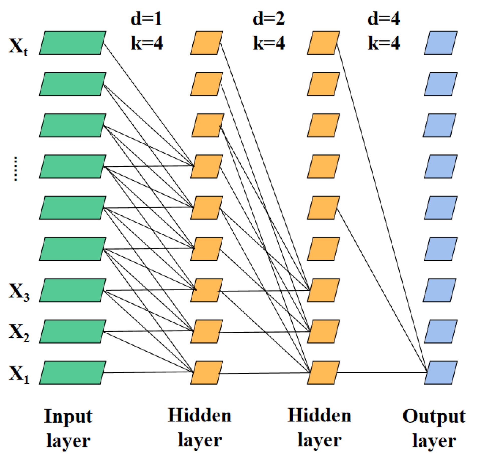
Then this paper used the aggregated spatial eigenmatrix as the input of the dilated convolution and used the stacked dilated convolution model to extract the time-dependent features of the two-dimensional eigenmatrix. Figure 4 is the architecture of stacked dilated convolution.

In Figure 4, stacked dilated convolution was connected to the local receptive field of the previous layer by feature mapping. First, the shared convolution kernel was adopted for operation, and then the eigenvalues were obtained by nonlinear calculation of the activation function. As shown in Figure 4, four data modules in the input layer were aggregated as a group for the first hidden layer through dilated convolution operation. The difference between dilated convolution and ordinary convolution lay in the introduction of the dilation rate, which allowed the convolution kernel to skip $d$ data modules with individual dilation rate in the processing step. As shown in Figure 4, the first dilation rate between input layer and the first hidden layer was set as 1, and the second dilation rate between the first hidden layer and the second hidden layer was 2. The third dilation rate between the second hidden layer and the output layer was 4, which meant the convolution kernel was sampled at 4 intervals. The unique structure of dilated convolution could obtain a larger receptive field without excessive network depth. This mechanism not only reduced space loss and information loss, but also made feature extraction more comprehensive. The dilated convolution formula is as follows.

$${(F*}_d{X\left)\right(x}_t)={\sum }_k^K{f}_k{x}_{t-(K-k)d}$$

(7)

In Formula (7), $f_k$ represents the filter and $x_t$ represents the characteristic sequence of input. Further, $d$ is the dilation rate, $k$ is the size of the convolution kernel, and $K$ represents the number of nodes participating in the dilated convolution operation in the local receptive field. The size of the receptive field of stacked dilated convolution was $\left(K-1\right)d+1$. By increasing the convolution kernel or dilation rate, the model could obtain a wider receptive field. According to [24], the initial values of convolution kernel, the network layer depth, and the dilation rate of stacked dilated convolution were set as 4, 4, and ${d=2}^i$, respectively, where $i$ is the network layer depth.

4. Experiment

4.1. Study Area and Dataset Description

With the rapid development of science and technology, air quality is being seriously affected by the emission of air pollutants from agriculture, industry, transportation and other activities. As the economic center of China, air pollution in Shanghai cannot be ignored. Therefore, Shanghai was selected as the research area in this paper, and the distribution of monitoring stations is shown in Figure 5. We chose station 2 as the target station for this article. Station 2 is located in the urban center and there are many air monitoring stations around it, so the prediction of the station could better reflect the influence of spatial-temporal correlation on the model prediction, as it was representative to a certain extent.

In this paper, hourly individual air quality index and meteorological data from 9 monitoring stations in Shanghai were collected from 26 August to 28 September 2013, and fused into original data sets. In order to facilitate the study of this paper, IAQI-PM_2.5 (the main estimation factor of air quality index) was taken as the research object of this paper. Original data were preprocessed with missing value imputation and outlier detection. Missing values within short time spans (i.e., in one hour or two hours) were interpolated with the first and second order Lagrange interpolation method. For missing values with a longer time span (i.e., in 5 h or more), these missing data were transferred from a nearby time period. If the time span was over 12 h, these records were considered as outliers, which were abandoned from the following experiments.

In the feature selection process, the Spearman rank correlation coefficient method was employed to identify and eliminate the features that were weakly correlated with IAQI-PM_2.5 in the original data set. The selected features included IAQI-PM_2.5, IAQI-PM₁₀, IAQI-NO₂, temperature, pressure, humidity, wind speed and weather. Detailed description of each feature is shown in

Table 1. Data set description.

Type	Feature Name	Data Type	Unit
Air quality data	IAQI-PM2.5	Numeric	None
	IAQI-PM10	Numeric	None
	IAQI-NO2	Numeric	None
Meteorological	Temperature	Numeric	°C
	Pressure	Numeric	hpa
	Humidity	Numeric	%
	Wind speed	Numeric	km/h
	Weather	Numeric	None

.

4.2. Parameter Tuning

4.2.1. Select the Data Partition Ratio

The prediction performance of the model was affected by different partition strategies of the original data sets. In order to improve the performance of the model, a random search method was used to find the optimal data set partition ratio. This paper divided data sets into the training set, verification set and test set. Different partitioning strategies, including (2:1:1), (3:1:1), (4:1:1), (5:1:1) and (6:1:1), were adopted. We used the idea of cross validation for each partition ratio of multiple tests. The average performance of multiple tests was taken as the final model performance of this partition ratio. The optimal partitioning strategy was selected by comparing multiple performance metrics (including RMSE, MAE, R²), as shown in

Table 2. The influence of different partition ratios on prediction performance.

Partition Ratio	RMSE	MAE	R2
2:1:1	13.721	10.747	0.839
3:1:1	11.142	8.072	0.893
4:1:1	10.8	8.622	0.901
5:1:1	10.468	8.340	0.902
6:1:1	14.499	10.239	0.818

.

It can be seen from the above table that when the data set partition ratio was (5:1:1), the ST-CCN-IAQI model achieved the optimal value of each performance metrics: RMSE was 10.468, MAE was 8.340, and R² was 0.902. As the proportion of training sets increased, the prediction performance of the model gradually improved. However, when the proportion of training sets was too large and the proportion of verification sets too small, it was not conducive to the air quality prediction of the ST-CCN-IAQI model. Therefore, the data set partition ratio was set as (5:1:1) for subsequent experiments.

4.2.2. Spatial Correlation Threshold

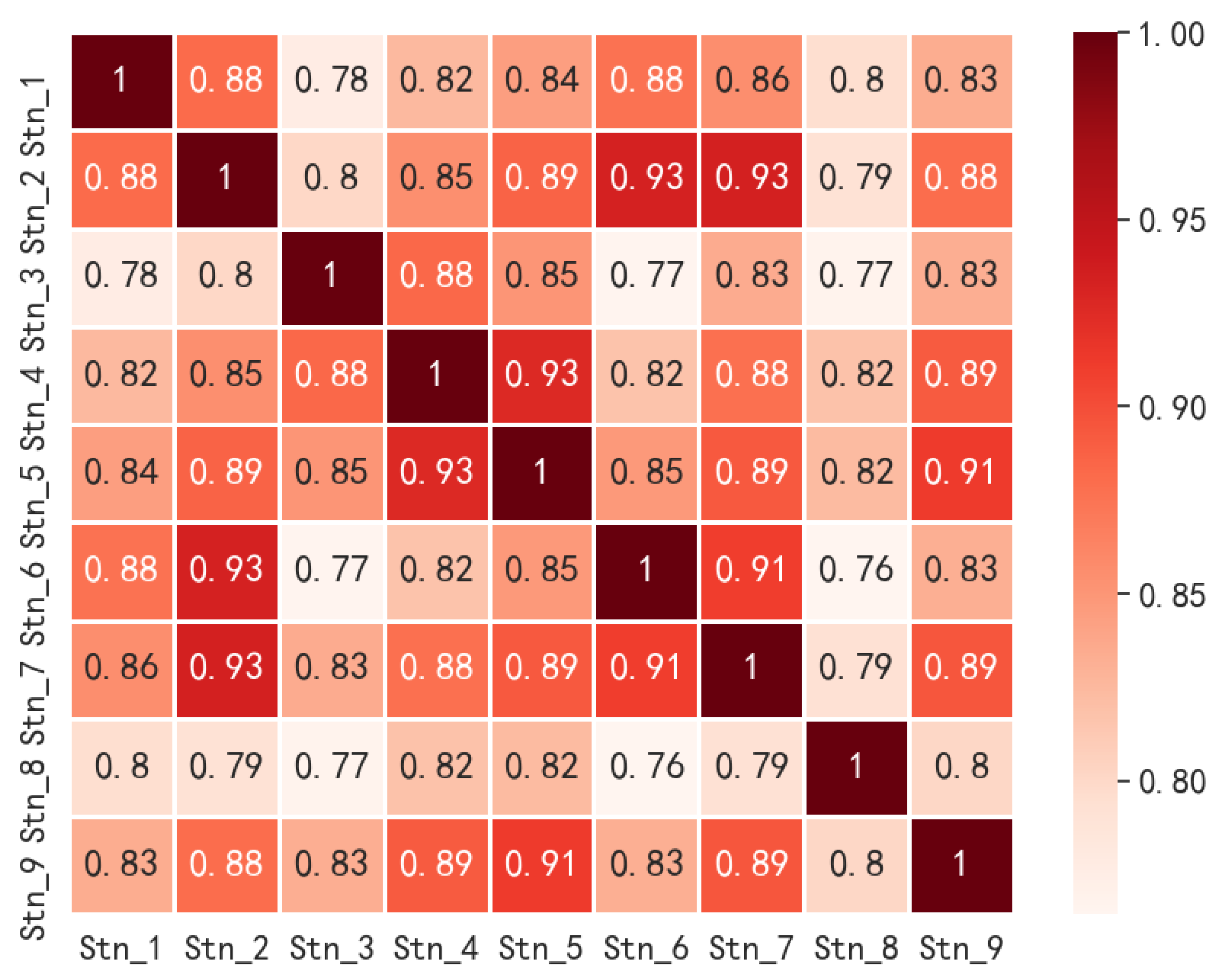
In the spatial feature extraction modeling mentioned above, we needed to set the correlation threshold to determine the monitoring stations to be included in the model prediction. In this paper, the correlation degree standard in statistics and correlation coefficient distribution were used to select the threshold. The correlation scale was 0.8 to 1 for highly strong correlation, 0.6 to 0.8 for strong correlation, 0.4 to 0.6 for moderate correlation, and less than 0.4 for weak correlation. We calculated the historical sequence (IAQI-PM_2.5) correlation between the target station (stn.2) and other stations by the Spearman rank correlation method. The correlation coefficient between stations is shown in Figure 6.

It can be seen from Figure 6 that the correlation coefficients between station 2 and other stations were almost all in the range of 0.8 to 1, indicating that station 2 had an extremely close relationship with other stations. For the study area of this paper, we set the correlation threshold to 0.8 to avoid the missing of strongly correlated spatial information. In the follow-up study, the threshold parameter in the spatial feature extraction module was set as 0.8.

4.2.3. Hyperparameter Tuning Based on Bayesian Optimization

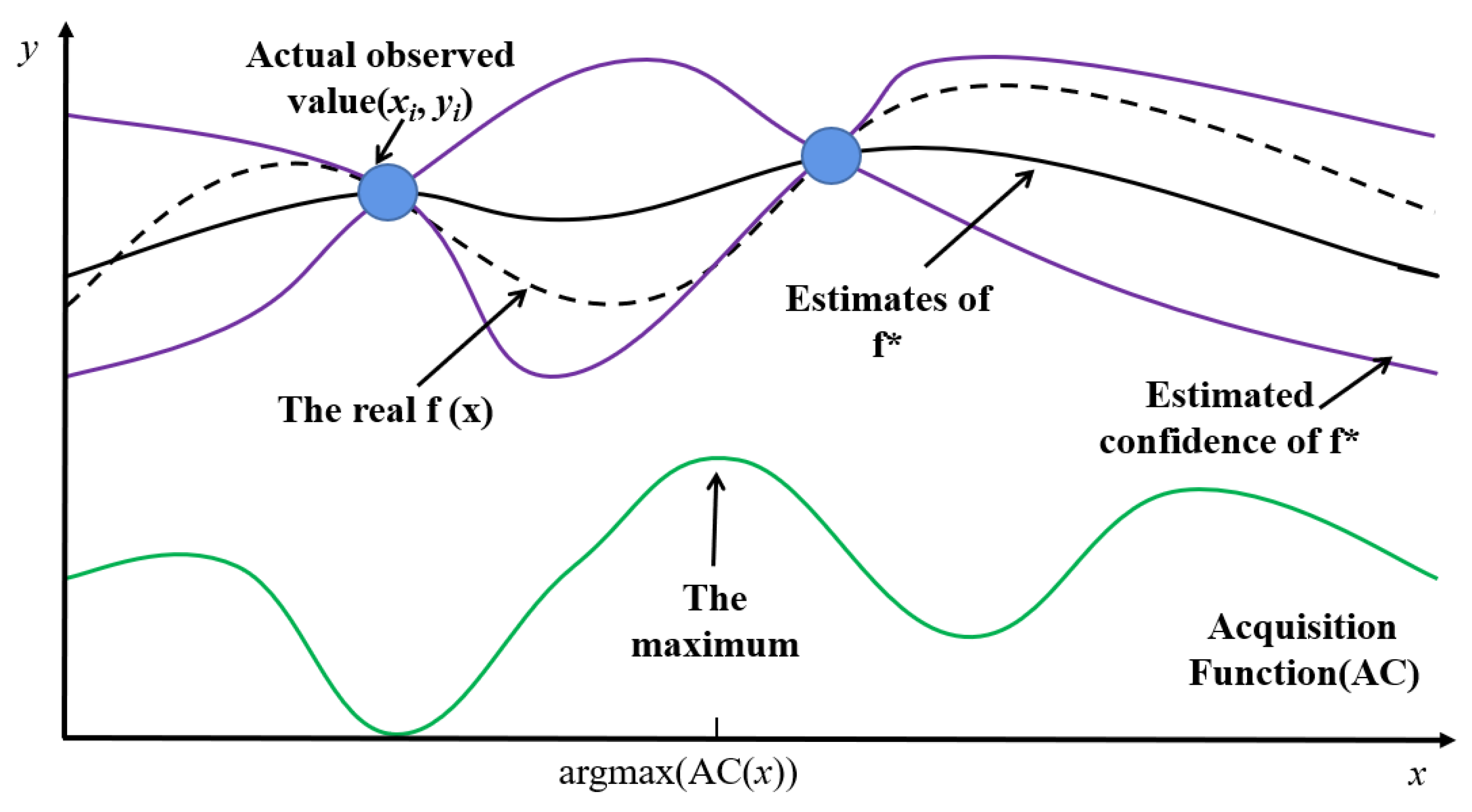
The performance of ST-CCN-IAQI was affected by many hyperparameters, such as network depth, number of hidden layer nodes and so on, as discussed in Section 3. Traditional empirical method and random search means need a lot of practical experience and cannot accurately obtain the global optimal hyperparameters. In this paper, the hyperparameters were tuned via Bayesian optimization [41]. Figure 7 shows the practical steps of Bayesian optimization.

The ultimate goal of Bayesian parameter tuning is to select a set of hyperparameters so that the loss function of the model can obtain the global minimum. For a black box model, we could not obtain its actual loss function. Only by calculating the approximate function and approximating the real loss function through continuous iteration could the hyperparameter combination which minimized the model loss value be obtained. In Figure 7, the horizontal axis represents the search space of the hyperparameter combination. The blue point represents known actual observations, namely ${(x}_i{,y}_i)$. Where, $x_i$ represents a group of hyperparameter values, and $y_i$ represents the loss function value obtained after model training. The black solid line is the estimated distribution of the function, and the region between the purple solid line is the confidence interval of the estimated function. The black dotted line represents the actual model loss function and the solid green line represents the acquisition function. First, based on the observation points, the Bayesian optimizer used the TPE process (probability proxy function) of the Gaussian mixture model to obtain the estimation function $f^{*}$ of the loss function $f\left(x\right)$. Secondly, the optimizer used the output of the probabilistic proxy model ($f^{*}$) to calculate the acquisition function, and selected the next observation point using the acquisition function. The acquisition function would measure the influence of observation points (sample points in the hyperparametric search space) on fitting $f^{*}$ and $f\left(x\right)$ to select the point with the greatest impact to perform the next observation. As shown in Figure 7, the maximum point $x$ of the acquisition function was calculated by the Bayesian optimizer, and then the group of hyperparameters represented by $x$ was put into the model for training, and the actual loss value $y$ was obtained. Finally, the new observation points $(x,y)$ were added to the known observation points. Through a certain number of iterations, the estimated function $f^{*}$ would gradually approach the actual loss function $f\left(x\right)$. The minimum point of $f^{*}$ calculated was the combination of hyperparameters after tuning.

Four hyperparameters, including hidden size, levels, kernel size, and dropout in stacked dilated convolution were tuned via Bayesian optimization. Hidden size represents the number of nodes in the hidden layer, levels represent the depth of the network layer, kernel size is the dilated convolution kernel, and dropout is the ratio of nodes removed randomly in each iteration.

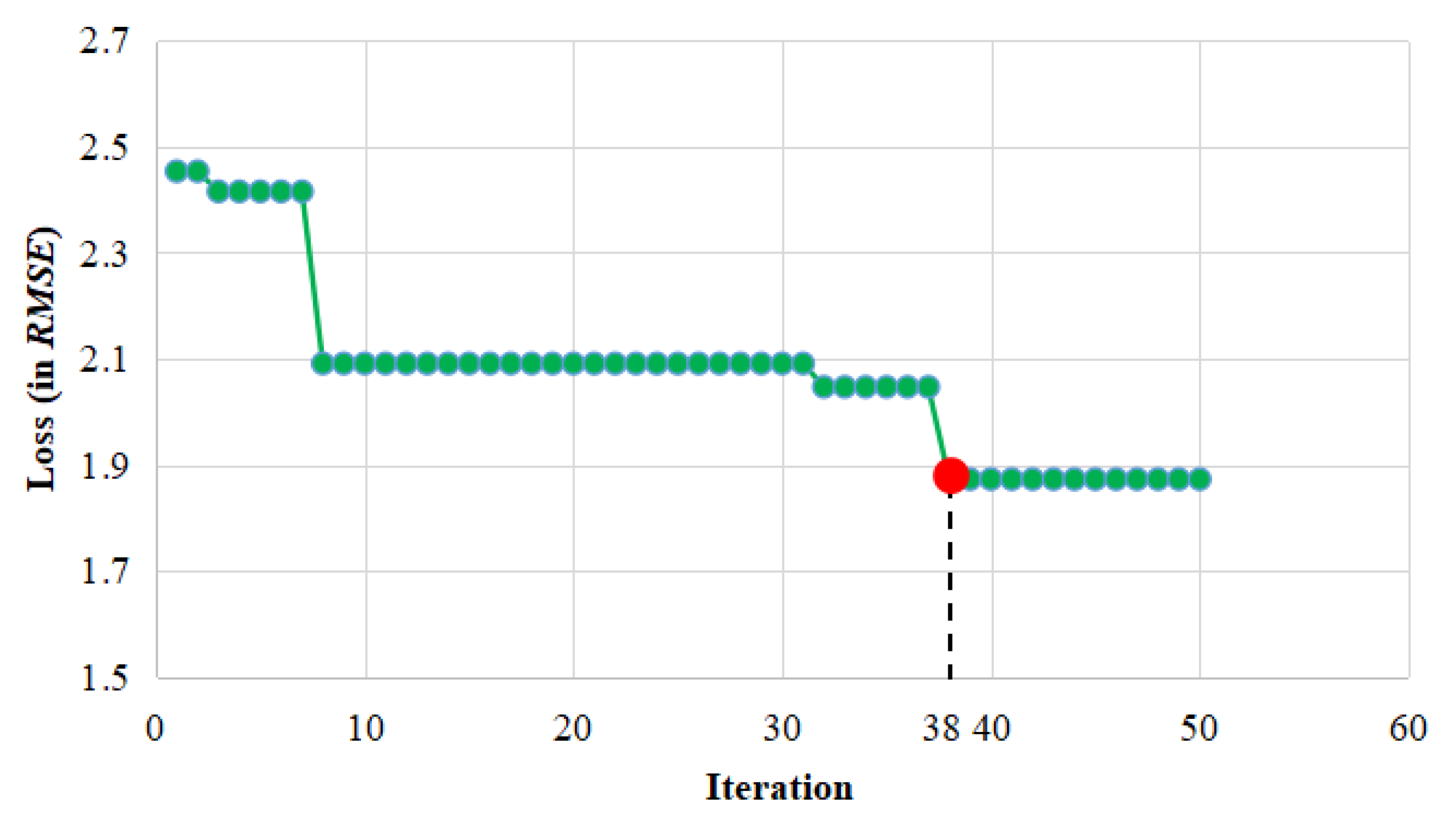
To run the Bayesian optimization process, RMSE was considered as Bayesian optimizer’s loss function. For the target station, it was obvious from Figure 8 that the Bayesian optimizer tended to converge after 38 iterations. For the sake of convenience, the number of iterations of the Bayesian optimizer was finally set to 50.

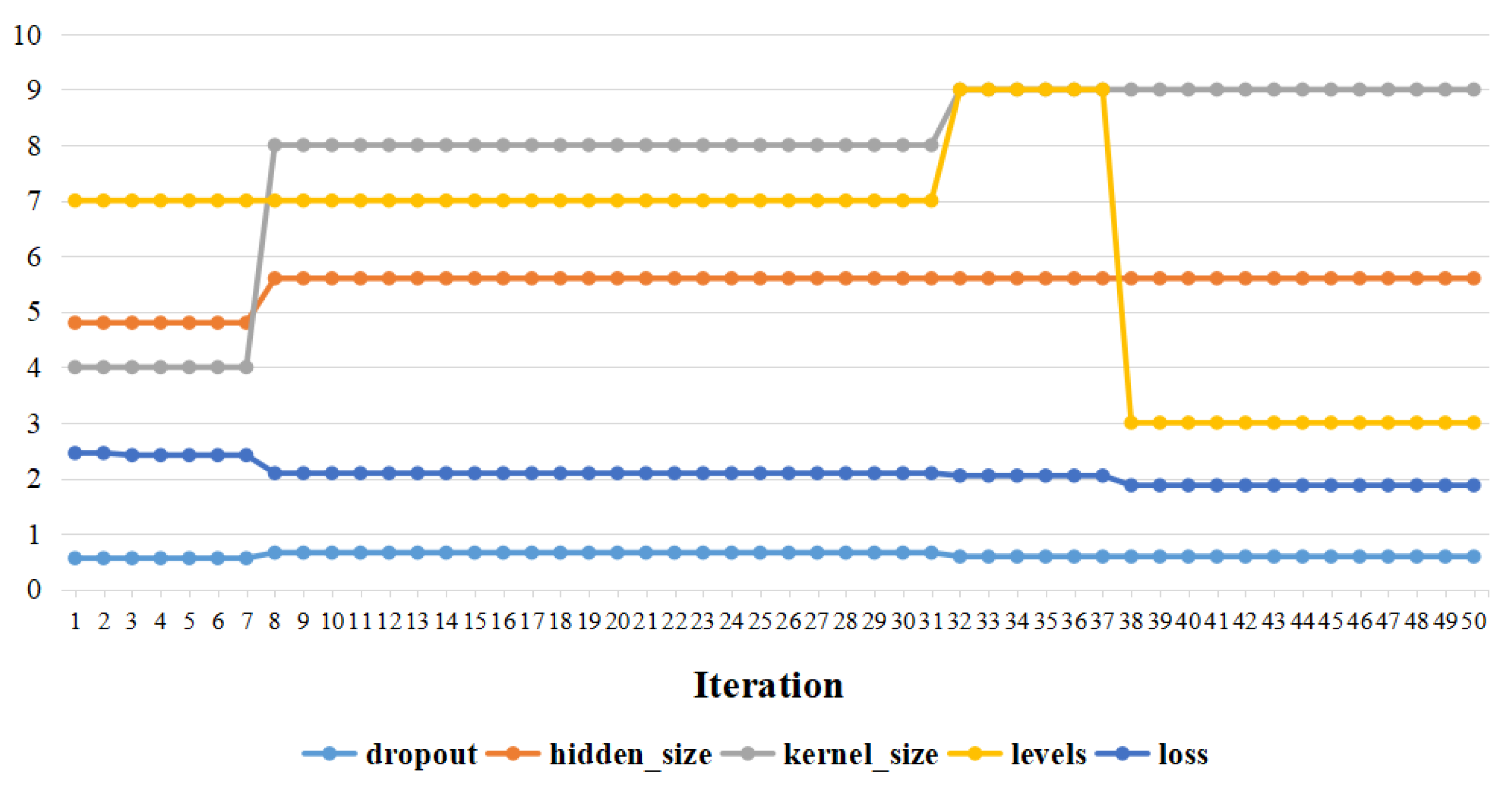
The initial searching space was as follows: Dropout values ranged from 0.5 to 0.9, and the step size was 0.01; Kernel size values ranged from 3 to 9, and the step was 1; Levels ranged from 3 to 9, and the step was 1; Hidden size values ranged from 48 to 64, and the step was 8 [24]. After 50 epochs, the values of four hyperparameters became steady. The final optimal values for ST-CCN-IAQI model were: $\mathit{dropout}=0.59$, $\mathit{hidden}\_\mathit{size}=56.0$, $\mathit{kernel}\_\mathit{size}=9.0$, and $\mathit{levels}=3.0$. Figure 9 shows the Bayesian optimization process of hyperparameters.

4.3. Prediction Performance Analysis

4.3.1. Target Station Performance Analysis

In this paper, a single monitoring station (stn.2) was taken as the target station to predict its IAQI-PM_2.5 at a future time. In order to demonstrate the advanced nature of the proposed model, a series of baseline models were compared with ST-CCN-IAQI. The baseline models included autoregression model, moving average model, autoregression-moving average model, artificial neural network, support vector machine regression, gated cyclic unit, long and short-term memory network and spatial-temporal graph convolution network. For the AR model based on stationary time series, an appropriate order $P=3$ was selected through $F$ test and an adaptive method was adopted to predict [42]. For the MA model, the order $P=3$ of the model was determined first, and then the autocorrelation between historical data and current data was determined for prediction [43]. The ARMA model, based on non-stationary time series, was determined through stationarity test, model recognition and test, and the order p and $q$ of the ARMA model were set to 5 and 6, respectively [25]. ANN could be regarded as a nonlinear mapping from the input space to the output space. ANN held two hidden layers, and each hidden layer contained 50 neurons, using ReLU activation function and Adam random gradient optimizer and other model parameters [31]. SVR selected appropriate function subset, discriminant function, RBF kernel function and parameter value $C=1000$ to complete prediction [34]. GRU model discarding rate was set to 0.2, hidden layer to 1 and hidden node number (16, 25) for the experiment [10]. LSTM model has a good retention effect on forward information, especially long-distance forward information. This experiment adopted three hidden layers, the number of nodes was 30, 50 and 70, and the learning rate was 1 [13]. A graph-based model called spatial-temporal graph convolutional network (ST-GCN) was also considered. The three-layer channels in ST-GCN block were 64, 16 and 64, respectively. We set the graph convolution kernel size K and time convolution kernel size Kt as 3 [19]. For linear statistical and temporal models, IAQI-PM_2.5 historical series were used as the input of the model. For shallow learning and deep learning models, we used the same feature sequence as the model input. In addition, the parameters of the above reference model were tested many times by using the general parameter configuration in the literature, and the parameters with the best prediction performance of the model were selected. Therefore, the parameter configuration adopted by the baseline model in this paper had a strong ability for generalization.

In this paper, MSE, RMSE, MAE and R² were utilized as evaluation metrics, and the performance of each model was obtained by five-fold cross -validation. For model comparison, the input dataset was divided into 5 subsets. One subset was adopted as the validation set, and the remaining four subsets as training sets. The average MSE, RMSE, MAE and R² from five-fold cross-validation were considered as the final performance for each model, as shown in

Table 3. Performance Comparison of each model (single station, stn.2).

Models	RMSE	MAE	R2
AR	12.366	8.397	0.888
MA	17.287	11.897	0.782
ARMA	12.504	8.477	0.885
ANN	13.032	9.030	0.876
SVR	12.821	8.554	0.880
GRU	12.883	8.829	0.878
LSTM	12.853	8.807	0.879
ST-GCN	12.621	8.713	0.884
ST-CCN	9.873	7.469	0.917

.

As shown in Table 3, ST-CCN-IAQI performed better than the baseline model in terms of RMSE, MAE and R² in the IAQI-PM_2.5 prediction task. On the whole, RMSE and MAE of ST-CCN-IAQI decreased by 24.95% and 16.87% on average, and R² increased by 5.69% on average compared with the baseline model. Compared with linear statistical and time series models, RMSE and MAE of ST-CCN-IAQI decreased by 28.03% and 19.93% on average, and R² increased by 8.03% on average. Compared with the shallow learning model, RMSE and MAE decreased by 23.55% and 14.98% on average, and R² increased by 4.44% on average. ST-CCN-IAQI was also significantly improved compared with deep learning model: RMSE and MAE decreased by 22.77% and 14.96% on average, and R² improved by 4.17% on average. The experimental results proved that the proposed model provides a potential research direction for fine-grained IAQI prediction. In order to compare each model intuitively, we drew a bar figure of model performance comparison.

By observing Figure 10a–c, it could be found that although the MA model had the worst performance, the results of traditional AR model and ARMA model were almost superior to all other complex models, such as ANN, SVR, GRU, LSTM and ST-GCN, both in terms of root mean square error (RMSE) and MAE. One possible explanation for this phenomenon is the strong periodicity of experimental data, which allows models based on linear and time series to better extract time dependence. The above experiments and analysis proved that ST-CCN-IAQI established a new baseline for IAQI-PM_2.5 prediction. In order to prove the robustness and stability of the model, we drew the prediction fitting figure of ST-CCN-IAQI for IAQI-PM_2.5 at a single station.

Figure 11 is the fitting figure of ST-CCN-IAQI prediction for IAQI-PM_2.5 of Station 2. For most of the time, there was a relative fit between the predicted value and the real value. However, due to the sharp fluctuations of IAQI-PM_2.5 at certain moments (140 and 360 in Figure 11), the predicted values occasionally had certain deviations. On the whole, the model had stable and accurate prediction performance in the stationary and non-stationary periods of IAQI-PM_2.5, which proved that the model has good robustness.

4.3.2. All Station Performance Analysis

The above experimental analysis proved that the ST-CCN-IAQI model had better prediction performance than the baseline in Station 2. In order to further verify the stable prediction performance of the model, ST-CCN-IAQI was used to predict IAQI-PM_2.5 of all stations in Shanghai. We used RMSE, MAE and R² as model evaluation indexes, and used the five-fold cross-validation method to obtain the prediction performance of the model for each station. The experimental results are shown in

Table 4. Comparison of prediction accuracy of all stations.

Stn.No	IAQI-PM2.5
	RMSE	MAE	R2
1	11.079	8.474	0.885
2	9.873	7.469	0.917
3	10.018	7.766	0.878
4	9.020	6.652	0.909
5	10.293	7.972	0.895
6	9.845	7.611	0.929
7	9.294	7.131	0.930
8	10.004	7.747	0.887
9	9.218	6.926	0.928
Average	9.849	7.527	0.906

.

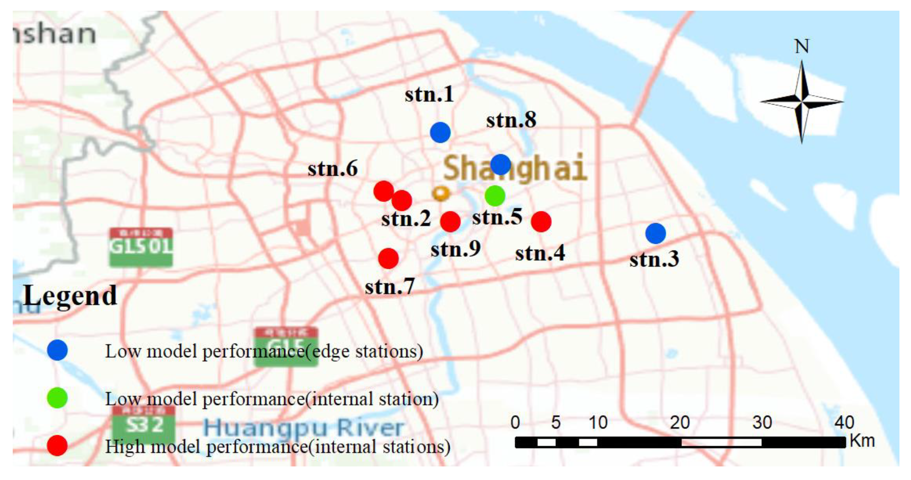
In Table 4, RMSE, MAE and R² of IAQI-PM_2.5 prediction of stations 7 and 9 were better than that of Station 2 selected in this paper, and the prediction error and fitting degree of other stations were also relatively good. After calculation, the average RMSE and MAE of the nine stations were 9.849 and 7.527, respectively, and the R² value was 0.906. Besides this, the fluctuation range of prediction error and goodness of fit of ST-CCN-IAQI model was small. The experimental results showed that the model had strong generalization ability and stability for IAQI-PM_2.5 prediction of different stations. In order to intuitively display the performance difference of the model in predicting air pollutants at each station, we drew the line figure.

As shown in Figure 12, the prediction effect of ST-CCN-IAQI model on IAQI-PM_2.5 of marginal stations (stations 1, 3, 8, etc., in Figure 5) was relatively poor compared with stations in densely distributed areas (stations 2, 6, 7, etc., in Figure 5). This means that in fine-grained IAQI predictive modeling, we should not ignore the spatial-temporal dependencies between stations. In addition, when ST-CCN-IAQI predicted IAQI-PM_2.5 of some internal stations (station 5 in Figure 5), the model had a large prediction error and deviation of fitting degree. One possible explanation lies in the more complex environmental conditions at station 5, which are susceptible to various external disturbances (traffic conditions, factory production, etc.). These factors may have led to some deviations in model predictions and should be taken into account in future IAQI prediction modeling.

4.4. Robustness Analysis

4.4.1. Significance Test

In order to identify whether ST-CCN-IAQI was significantly superior to other baselines in fine-grained IAQI prediction, we adopted the Friedman’s test, a non-parametric statistical method which can measure the difference among all models, to further explore the robustness of the proposed model.

Three test datasets for Friedman’s test were constructed as follows. For the historical data set of each station, data were extracted from the upper quartile, median, and lower quartile positions, and each position extracted 10% of the original dataset (5% of the original dataset was extracted before and after each quartile, respectively). Data extracted from each location constituted three datasets: data_25%, data_50%, and data_75%.

The Friedman test was performed, based on the three constructed datasets, on all nine models. First, the nine models were trained with the three datasets to predict the PM_2.5 of a single monitoring station (stn.2), and the RMSE values of different models were obtained. Second, the average ranking value of the nine models were obtained based on RMSE results from these three datasets, as shown in

Table 5. RMSE index ranking of 9 models in 3 data sets.

	AR	MA	ARMA	ANN	SVR	GRU	LSTM	STGCN	STCCN
data_25%	12.35(2)	17.12(9)	12.57(3)	13.03(8)	12.81(5)	12.87(7)	12.84(6)	12.61(4)	9.85(1)
data_50%	12.47(2)	17.67(9)	12.63(3)	13.12(7)	12.92(5)	13.12(7)	13.04(6)	12.76(4)	9.96(1)
data_75%	12.15(2)	17.43(9)	12.45(3)	12.93(7)	12.85(6)	12.97(8)	12.77(5)	12.68(4)	9.62(1)
Average	2	9	3	7.3	5.3	7.3	5.7	4	1

. Finally, the null hypothesis H0 was: there is no significant difference in RMSE between ST-CCN-IAQI and other baseline models, and the hypothesis was tested by calculating ${\chi }_F^2$ and $F_F$. in Formulas (8) and (9).

$${\chi }_F^2=\frac{12N}{k(k+1)}[{\sum }_j^{}{R}_j^2-\frac{{k(k+1)}^2}{4}]$$

(8)

$$F_F=\frac{{(N-1)\chi }_F^2}{{N(k-1)-\chi }_F^2}$$

(9)

As shown in Formulas (8) and (9), $N$ and $k$ represent the number of independent data sets and the number of models, respectively, and $R_j$ represents the average ranking of performance indicators of the j-th model in different data sets.

As shown in Table 5, the RMSE index ranking of the nine models from three datasets was calculated with ${\chi }_F^2=23.62$ and $F_{F }=125.06$ and $F_F$ follows (8,16) degrees of freedom. When the confidence level α = 0.05, the critical value of $F (8,16)$ was 2.59. Obviously, the $F_F$ value related to RMSE index ranking was greater than the critical value 2.59. Therefore, the previous null hypothesis was rejected, which proved that the prediction performance of the ST-CCN-IAQI was significantly different from other baselines.

4.4.2. Model Generalization Analysis

In order to verify the stability of the proposed model in a wider spatial-temporal span, we made IAQI predictions for each station over the next 24 h. Ten predictions were made for each hour on each station. IAQI-PM_2.5 values of each station were predicted in hours, the average of 10 predictions for each hour were compared with real series in a violin plot. The experimental results of all stations were $X\in R^{S\times H\times T}$, where $S$ represents the number of monitoring stations, $H$ represents different moments, and $T$ represents the number of tests. We compressed the three-dimensional matrix from the S-axis and reduced the experimental results to two dimensions, that was, $X_{\mathit{new}}\in R^{H\times T}$. The dimension reduction was to facilitate the display of the average prediction interval and to show the changing trend at all hour points. Figure 13 is the violin plot drawn after dimension reduction.

Figure 13a shows the fluctuation range and evolution trend of IAQI-PM_2.5 predictions in the next 24 h. In order to intuitively illustrate the statistics contained in the violin figure, this paper drew a violin subplot at 0 o’clock, as shown in Figure 13b. The violin subplot consists of a fusion of nuclear density and boxplot. For each violin subplot, the inside is a boxplot and the outside is surrounded by a kernel density figure. The kernel density figure visually shows the prediction distribution. The upper and lower bounds of the black line segment represent the inner and outer limits, the upper and lower boundaries of the black rectangle represent the upper and lower quartiles, and the white points in the black rectangle represent the median in the sample. As shown in Figure 13a, it could be seen intuitively that the 24-h IAQI-PM_2.5 value fluctuated within a stable range. The predicted values were distributed near the real values with high probability, which proved the robustness and stability of the model. In addition, the blue line represents the mean of the 10 predictions and the red line represents the true value. It could be seen that the error between the predicted mean value and the real value in periods 7–10 and 13–16 was large, and the predicted mean value and the real value at other times were fitted. This indicated that the external factors leading to the drastic fluctuation of IAQI had a great impact on the prediction performance of the model. From the changing trend of IAQI-PM_2.5, from 0 h to 7 h, there was very little human activity, which reduced the anthropogenic emissions of PM_2.5. With the transport and diffusion of meteorological factors, IAQI-PM_2.5 gradually decreased. From 7 h to 16 h, IAQI-PM_2.5 rose step by step. At this time, due to the impact of human activities, such as traffic exhaust emissions and factory production activities, PM_2.5 gradually accumulated and could not be dispersed in a timely manner. After 18 h, the value of IAQI-PM_2.5 kept at a high level. During this period, most factories had closed, resulting in a significant reduction in PM_2.5 emissions. However, as it was still in the evening peak when people get off work, the concentration of PM_2.5 remained high, due to heavy traffic exhaust emissions. Therefore, most of the multiple peaks in the figure came from traffic exhaust emissions, industrial production and coal emissions. It could be seen that the peak period of IAQI-PM_2.5 overlapped greatly with the period of human activities, which caused a very serious threat to the safety of human life. In order to protect urban ecology and human health, this paper advocates low-carbon travel for human beings and minimized activities at night (in order to avoid long-term exposure to high concentrations of PM_2.5). In addition, the government should strengthen the control and regulation of industrial exhaust emissions and coal-fired emissions in cities.

4.5. Impact Factors’ Influence Analysis

In this paper, air pollutant data and meteorological data were selected as input features. It is believed, from literature, that atmospheric environmental factors do have different degrees of influence on IAQI-PM_2.5 prediction [39,40]. However, how to quantify the impact factors’ influence still remains in something of a mist. Shapley analysis was then employed to quantitatively analyze the positive and negative gain of input features on model prediction from local and global perspectives.

Shapley analysis belongs to post interpretation to identify whether the predicted value given by the model has a certain relationship with the input features. All input features were treated as contributors and the contribution of the input features were estimated according to the predicted values. For each predicted sample (containing multiple input features), the black-box model produced a predicted value, and Shapley process calculated the influence weight for each feature (that is, the analysis result of Shapley). Then, the Shapley results could be explained locally from a single prediction sample, or globally from all predicted samples. Figure 14 shows the local perspective of Shapley analysis from a single dataset sample.

In Figure 14, the horizontal line represents the weight values of influence, and the vertical line represents each input feature. The value $f\left(x\right)$ represents the value of one prediction after considering all input features, and $E\left(f\right(x\left)\right)$ represents the mean value of multiple predictions. The red bar shows how much a particular feature increased the predicted value, and the blue bar shows how much a particular feature decreased the predicted value. In the local perspective, this feature of IAQI-PM₁₀ had the maximum forward gain for IAQI-PM_2.5, which increased the predicted value by 30.95. Atmospheric pressure and temperature had a significant negative gain for IAQI-PM_2.5, which reduced the predicted value by 7.25 and 4.8, respectively. The other features had relatively little influence on the output features. Local perspective analysis can accurately and intuitively obtain the influence weights of input features in a single sample, but it is limited to the one-sidedness of the output results of a single sample.

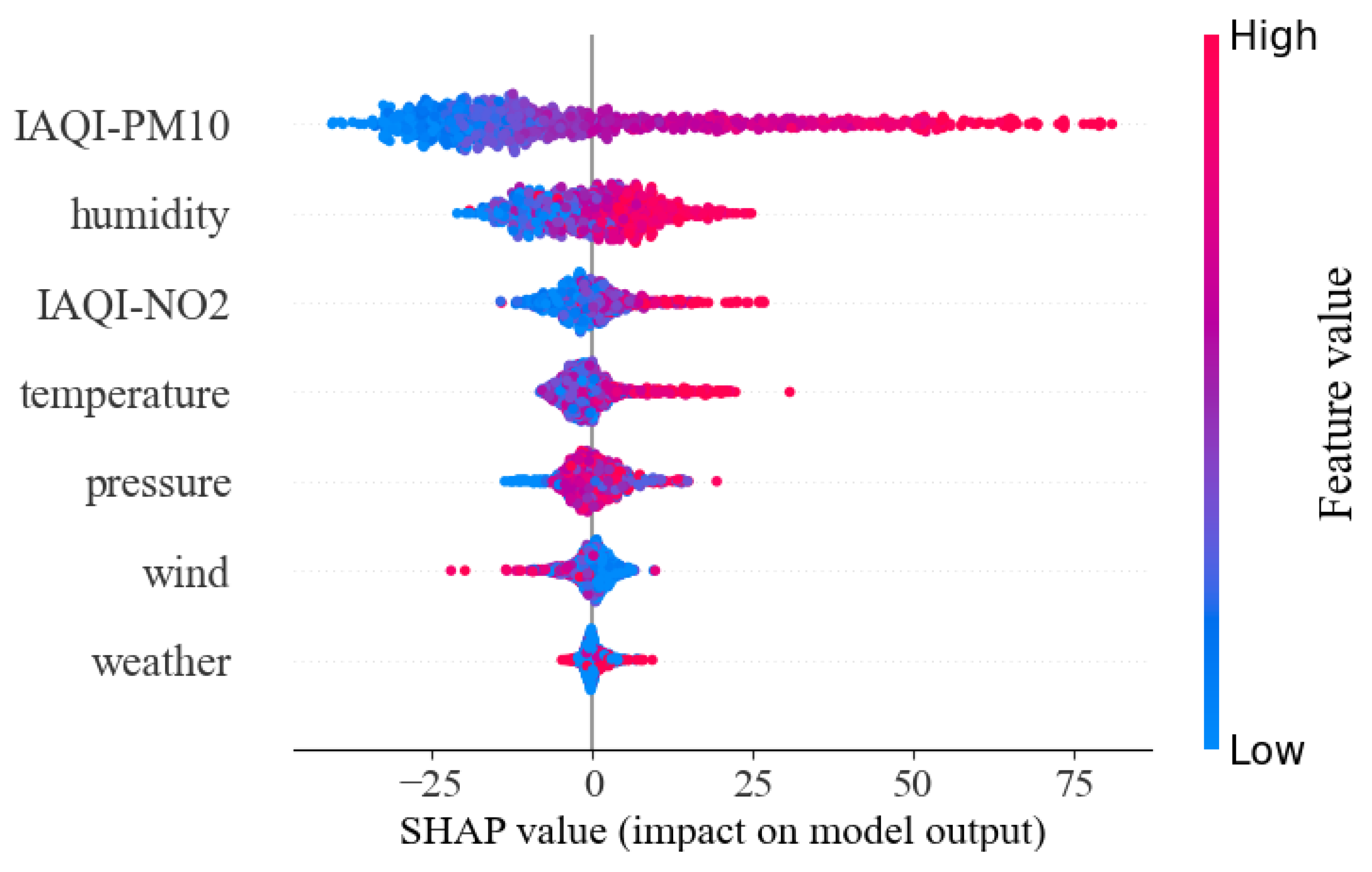
In order to obtain the effect weights of input features for output space, the global perspective of Shapley analysis from all samples was also carried out, as shown in Figure 15.

Figure 15 shows the influence weights of input features on IAQI-PM_2.5 prediction from all samples. The horizontal line represents the influence weight of a specified feature on the output, the left vertical line represents different features, and the right vertical line with different colors represents the level of features’ weights. The features’ weights stand for the importance for the final output, which were ranked in a descending manner. The first three significant impact features were the IAQI value of PM₁₀ (IAQI-PM₁₀ in Figure 15), humidity and IAQI-NO₂, while the left four features, viz. temperature, pressure, wind speed and weather, held relatively weak influence for IAQI-PM_2.5 prediction. The IAQI-PM₁₀ and IAQI-NO₂ did have a strong positive effect along with IAQI-PM_2.5. One possible explanation is that PM_2.5, PM₁₀ and NO₂ are the main pollutants of traffic exhaust emissions and factory production, and the coupling effects among these pollutants cannot be neglected. This phenomenon is also demonstrated in physicochemical models of air pollution [22,23]. Humidity held both positive and negative effects for IAQI-PM_2.5 prediction. When humidity was high, humidity behaved positively with IAQI-PM_2.5 prediction and vice versa, which may seem counterintuitive. According to actual meteorological data in Haikou, one reasonable interpretation lies in the fact that that higher humidity is more conducive to PM_2.5 suspension and retention in the air, while lower humidity makes for better transportation of PM_2.5 in cool air. Figure 15 implies that air pollutants (i.e., PM₁₀, NO₂) and meteorological factor (i.e., the humidity) should not be neglected in the modeling of IAQI-PM_2.5 predictions.

5. Discussion

5.1. The Influence of Spatial Effect on Prediction Results

In our experiments, the prediction results of IAQI at different stations showed a large difference. A station’s spatial distribution pattern plays a crucial role which cannot be neglected. When a monitoring station was located in the dense downtown area, the prediction performance was usually better compared with that of an isolated station (or an edge station). This phenomenon is illustrated in red spots and blue spot in Figure 16.

As shown in Figure 16, some stations located in dense areas showed the performance that was still relatively poor, as shown in Figure 16 (the green spot). One possible reason is that IAQI-PM_2.5 is susceptible to many external uncertainties (traffic conditions, human activities, etc.). To sum up, comprehensive spatial correlation characteristics and various spatial effects should be incorporated into IAQI prediction modeling.

5.2. The Influence of Multi-Source Factors on Prediction Results

In the previous paper, Shapley analysis quantified the influence of multi-source factors on the prediction results of the model. As shown in the experimental results, the degree of interaction between air pollutants was significant, and some meteorological factors also had an important impact on IAQI. The experimental results were consistent with common sense, because physical and chemical reactions between air pollutants can change the concentration of air pollutants. Meteorological factors, such as wind direction, wind speed, air temperature, air pressure and so on, play an important role in the transport, diffusion and dilution of air pollutants.

Experimental analysis has proved that the integration of multi-source influence factors in modeling has a positive driving effect on model prediction. Therefore, multi-source impact factors are the basis for precise and fine-grained IAQI prediction. In future work, we should identify as many important influencing factors as possible and incorporate them into IAQI modeling.

However, some influencing factors, such as topography and features, were still not considered in this paper. In cities, tall buildings create eddies in the moving atmosphere. It is difficult for air pollutants to escape in eddy zones, which are completely polluted, so similar conditions can occur in hills or valley basins. In addition, traffic conditions in urban areas also lead to a large number of pollutant emissions, including particulate matter (PM), CO, CO₂, NO_x, etc. These factors provide some new directions for IAQI prediction.

5.3. Advantages of ST-CCN Compared with Typical Deep Learning Models

At present, the popular models in the field of IAQI prediction are RNN-based models and graph-based models. However, the models based on RNN have some disadvantages, such as gradient disappearance and gradient explosion, and are iteration propagation time consuming and require large memory. There are also many unstable factors in graph-based models, such as artificially defining the relationship between variables, Markov hypothesis to explain the interaction between variables, and difficulty in capturing the edge relationship between stable nodes. The ST-CCN-IAQI model proposed in this paper overcomes the problems of the above model. Convolutional neural networks can capture stable spatial distribution features. Stacked dilated convolution can capture long time efficient time features with small memory requirements and avoiding of gradient problems. Secondly, ST-CCN-IAQI optimizes the convolutional neural network for air pollutant spatial feature extraction based on spatial attention mechanism. The time attention mechanism is used to make stacked dilated convolution pay more attention to time dependent periods. The introduction of spatial-temporal attention mechanism enables ST-CCN-IAQI to have stronger spatial-temporal feature extraction ability compared with deep learning model.

In conclusion, the ST-CCN model proposed in this paper provides an open framework. Compared with the model based on RNN and graphs, ST-CCN can conveniently incorporate multi-source influencing factors and multiple convolution structures into the prediction modeling of air pollutants.

6. Conclusions

In the past few decades, the rapid development of urbanization has led to an increasingly serious problem of air pollution, especially in China. In order to promote the sustainable development of urban public health and society, it is necessary to make fine-grained, accurate and effective prediction of air quality Index (AQI). As individual air quality index (IAQI) is the basis of AQI estimation, accurate and fine-grained IAQI prediction has become an important research direction in the field of air pollutant prediction. However, IAQI predictions still face significant challenges due to the complexity of meteorological processes and influencing factors.

In this paper, the prerequisites for IAQI prediction modeling were analyzed, including the spatial-temporal correlation between monitoring stations, air pollutants and meteorological factors. We further reviewed the limitations of traditional and deep learning-based methods for IAQI prediction. We incorporated air pollutants and meteorological factors into IAQI modeling, and considered the spatial-temporal dependence between air monitoring stations. In order to overcome the disadvantages of traditional spatial-temporal modeling methods, we applied convolutional neural network and causal convolutional network to extract spatial-temporal features, and then proposed the ST-CCN-IAQI model.

ST-CCN-IAQI is divided into two parts: the first part is space feature extraction. We used Spearman correlation analysis, convolutional neural network and spatial attention mechanism to extract spatial correlation features. The second part is time feature extraction. We integrated time attention and stack dilated convolution to extract time dependent features for single-step prediction. We obtained the historical data with a longtime span by setting the expansion factor, expanding the receptive field, avoiding space waste and information omission, and improving the prediction performance.

Based on the above modeling process, we further optimized the parameters to improve the performance of the model. Firstly, the threshold was selected through correlation analysis and correlation intensity measurement standard. Secondly, we used the Bayesian tuning method to improve the learning rate, expansion convolution kernel, sliding window and other parameters of the model. Finally, the optimized hyperparameter combination was applied to the subsequent prediction practice.

In order to facilitate the testing of the model proposed in this paper, IAQI-PM_2.5 (PM_2.5 is the main air pollutant) was adopted as the research object in this paper. We compared ST-CCN-IAQI performance with a series of baseline models, including AR, MA, ARMA, ANN, SVR, GRU, LSTM, and ST-GCN. We used RMSE, MAE, and R² to evaluate performance. We conducted a series of experiments on a single monitoring station (Station.2) and all monitoring stations. The final results showed that:

• In the IAQI-PM_2.5 prediction task of a single station, ST-CCN-IAQI performed better than the benchmark model in RMSE, MAE and R². On the whole, RMSE and MAE of ST-CCN-IAQI decreased by 24.95% and 16.87% on average, and R² increased by 5.69% on average compared with the baseline model. Compared with linear statistical and time series models, RMSE and MAE of ST-CCN-IAQI decreased by 28.03% and 19.93% on average, and R² increased by 8.03% on average. Compared with the shallow learning model, RMSE and MAE decreased by 23.55% and 14.98% on average, and R² increased by 4.44% on average. ST-CCN-IAQI was also significantly improved compared with deep learning model: RMSE and MAE decreased by 22.77% and 14.96% on average, and R² improved by 4.17% on average.
• For all stations, the mean RMSE and MAE of ST-CCN-IAQI model were 9.849 and 7.527, and R² was 0.906. The average prediction accuracy of the model for all stations was close to that of the single station, and the fluctuation range of the model’s prediction error and goodness of fit was stable. The above results proved that the model has strong generalization ability and stability for IAQI-PM_2.5 prediction of different stations.

To further test the model’s progressivity and robustness, we first analyzed the performance difference between the model and the baseline using the Friedman test, and proved that the model was significantly superior to the baseline model. Secondly, we used the model to predict the IAQI-PM_2.5 of all stations in the next 24 h. The robustness of the model was proved by many tests on all stations at different times.

In addition, Shapley analysis quantified the influence of various input features on the prediction results of the model. The results were consistent with human cognition. In practical forecasting tasks, incorporating important influencing factors into modeling can effectively improve the prediction performance of the model.

This paper also discussed the influence of spatial effect and multi-source factors on the prediction performance of the model. After analysis, it was proved that IAQI modeling is necessary and effective to consider these factors. In addition, from the theoretical aspect of model architecture, the advantages of CCN model compared with RNN model were analyzed, and it was proved that CCN is more suitable for IAQI sequence prediction task.

There are still some limitations to this study. First, when the sample data set was too small, the temporal and spatial causality model in this paper did not perform well. Secondly, we only used this model to make a single-step prediction for IAQI, and multi-step prediction research for IAQI will be further carried out in the future.