Article

Precipitation and Temperature Climatologies over India: A Study with AGCM Large Ensemble Climate Simulations

1
Disaster Prevention Research Institute, Kyoto University, Gokasho, Uji, Kyoto 6110011, Japan
2
Earth Science Center, Japan Meteorological Corporation Limited, Osaka 5406017, Japan
3
Research Institute for Global Change, Japan Agency for Marine-Earth Science and Technology, Yokohama 2360001, Japan
*
Author to whom correspondence should be addressed.
Atmosphere 2022, 13(5), 671; https://doi.org/10.3390/atmos13050671
Submission received: 25 February 2022 / Revised: 7 April 2022 / Accepted: 20 April 2022 / Published: 22 April 2022
(This article belongs to the Section Climatology)

Abstract

:
This study investigated the precipitation and temperature climatologies over India from large ensemble (100 members) historical climate simulations in two recent past climate periods (1951–1980 and 1981–2010). The main focus was to statistically examine the usefulness of such large historical climate simulations by discussing (1) the precipitation and temperature climatologies and their distribution patterns, (2) the annual cycle of the temperature and precipitation climatologies, and (3) the frequency distributions and potential spatial patterns of climate variability. We applied empirical orthogonal function to understand the characteristics and normal probability distribution function to investigate the frequency. Results indicated good agreements of these large ensembles simulated results with the observation over Indian region. The precipitation amount over many regions of India is decreased and temperature over entire India is increased in 1981–2010 compared to that in 1951–1980. The annual cycle of the precipitations over India indicated a decrease of the precipitation amounts from June through October, while an increase of precipitation for the months from November through January. The annual cycle of the temperature over India indicated an increase of temperature during July through March. The frequency distributions of monthly precipitations and temperatures indicate an overall decrease of precipitation and an overall increase of temperature in recent climate period. The reason of decreased precipitation in recent climate period is attributed to a decrease of relative humidity and cloud together with weaker vertical velocity over Indian region during 1981–2010. Overall study validates the usefulness of these large ensemble climate simulations for the assessment of climate over India and suggests that these datasets may be used for various purposes related to weather and climate over India.

1. Introduction

Climate change is one of the main concerns in our lives today, which has attracted the attention of the global community and its impact is being felt by global warming and changing precipitation. According to the recent reports of the Intergovernmental Panel on Climate Change (IPCC) the global mean surface temperature is increased by 0.85 °C during 1880–2012 and the mean precipitation has increased over mid-latitude areas of the Northern Hemisphere since 1901 and decreased over other latitude areas [1,2]. As a consequence, the economic and social challenges occur around the world such as damage of infrastructure, industry losses, health problems, and agricultural losses [3]. Therefore, assessing the past and future patterns on temperature and precipitation distribution has become major concern now-a-days in order to assess socioeconomic impact of the climate change. Several studies have assessed various methods such as periodogram, autoregressive integrated moving average, vector autoregression etc. to model and predict the temperature and precipitation climatology over many regions across the globe [4,5,6]. In a recent study, Akdi and Ünlü [4] identified the hidden cycles of precipitation and temperature by employing periodogram-based time series methodology. In numerous studies, the empirical orthogonal function (EOF) analysis is used to depict the variations of precipitation and their distribution with time [7,8].
The climate signals over India during the 20th century show an increasing trend in surface temperature by 0.4 °C and a change in the spatial distribution of precipitation [9]. However, the surface temperature and precipitation distribution patterns over the India are not uniform and vary on seasonal scales and are largely modified by the altitudes, locations and geographical features. In a recent study, Nayak et al. [10] highlighted that the 30-years (1981–2010) mean annual temperature corresponds to 23.15 °C over India, while the seasonal temperature varies in the range from 16.83 °C in winter (December–January–February) to 26.43 °C in monsoon (June–July–August–September). Kishore et al. [11] reported that the region of India received about 99 mm/month amount of mean precipitation during 1989–2007 in annum, which is ~330 mm/month in monsoon and about 52 mm/month in autumn (October–November). Past researches also reported a change pattern of precipitation over India. Dey and Mujumdar [12] highlighted that the precipitation homogeneity over India significantly changed in recent past periods (1951–2010) both in the amount and timing. Goswami et al. [13] documented that heavy (>100 mm/d) and very heavy (>150 mm/d) precipitation events during 1951–2000 over central India significantly changed. Several studies (e.g., [13,14,15]) also highlighted the trends of the precipitation associated with the Indian monsoon over different regions across India. Sinha Ray and Srivastava [16] documented an increase trend of the precipitation in monsoon season over certain Indian regions. On the other hand, Dash et al. [17] reported a decrease in trend in the mean monsoonal precipitation over whole India. All these studies clearly indicate that the climatology pattern over India shows a variety of trends in regional, seasonal and annual distributions.
Although a large number of studies [10,11,14,15,18,19,20,21,22,23,24,25,26,27,28,29,30,31,32,33] have investigated the temperature and precipitation pattern and climatology over the Indian regions from observation, reanalysis and model datasets, most of them have discussed the monsoon precipitation features from a single model. However, in recent decades, the climate studies have favored to consider multi-model ensemble strategy, particularly to understand the associated climatology uncertainties (e.g., [34]) because different models have different strengths and weaknesses in the model formulation. The different source of the uncertainty in the climate simulations can be model uncertainty, internal variability and/or scenario uncertainty [35,36,37,38]. Because the climate system is chaotic, so a small change in the initial condition or perturbations may bring a different path for the whole system. Therefore, the precipitation and temperature climatologies and their distributions from ensemble analysis provides a better understanding of uncertainty in the climate simulations [34,39,40]. It is therefore highly desirable to understand the salient features of the climatology over India from ensemble climate simulations in order to assess the uncertainties in the context of climate risk management.
Recently, Mizuta et al. [41] performed large ensemble global climate simulations with 100 experiments for present climate (1951–2010) at 60 km spatial resolution by using Meteorological Research Institute (MRI) Atmospheric General Circulation Model. Several recent studies (e.g., [42,43]) have used these large ensemble climate simulation products to predict the past climate over different regions across the globe and confirmed the model’s reproducibility in capturing various aspects of the climate. In this sense, these large ensemble climate products should provide new insights into climate change assessment over India in order to reduce the uncertainties in the context of climate risk management. In addition, application of such large ensemble climate simulations may be useful to reveal and better characterization of other climatic features over India not only for past climate, but also for the future developmental planning and decision making. We thus attempted to investigate the precipitation and temperature climatologies from these large ensemble (100 members) climate simulations during recent past periods (1951–2010) to explore the usefulness of these products over India by discussing (1) the temperature and precipitation climatologies and their distribution patterns, (2) the annual cycle of the temperature and precipitation climatologies, and (3) the frequency distributions and potential spatial patterns of climate variability. Section 2 provides the detailed description of the data and methods. The results of the temperature, precipitation and other environmental climatologies are given in Section 3. The related discussion and conclusions drawn from this study are presented in Section 4.

2. Materials and Methods

We analyzed the hourly precipitation and daily temperature datasets of the large ensemble (100-members) historical climate simulation products [41]. This dataset was simulated by the AGCM model at 60 km-mesh over the globe for the period 1951–2010. These simulations are conducted with various initial conditions and tiny perturbations in sea surface temperatures for 6000 historical years. Here the 6000 years comprise with 100 ensemble experiments for 60 years each. The Centennial observation-based estimates of sea surface temperature, sea ice concentration, and sea ice thickness are forced as lower boundary conditions. The initial conditions are provided from the snapshots at different times obtained through separate simulations using the same AGCM model. The details of these experiments are described in Mizuta et al. [41]. This dataset is known as d4PDF data (the database for Policy Decision making for Future climate change) and a brief description of this dataset is given in the Data Integration and Analysis System (DIAS) data catalog (http://search.diasjp.net/en/dataset, accessed on 10 February 2020). We also used India Meteorological Department (IMD, https://mausam.imd.gov.in/, accessed on 20 November 2016) gridded daily observation (0.25° × 0.25° for precipitation and 1° × 1° for temperature) for the period 1951–2010 to validate the model simulated climatologies. In methods, we first divided the whole period (1951–2010) into two present-day climate periods viz. 1951–1980 and 1981–2010 and derived the climatologies, annual cycles and frequency distributions from each AGCM ensemble simulations and that of from IMD observations for the said two climate periods over the study region ‘India’ (the region is highlighted in Figure 1).
The normal probability distribution function (PDF) is used to describe the variabilities of monthly precipitation and temperature. We used this PDF based on the temperature and precipitation results of a previous study [44] where a number of coupled climate models were evaluated through the PDFs.
The changes in the precipitation and temperature patterns through their spatial distribution, annual cycles and frequency distributions are explored in recent climate period (i.e., 1981–2010) compared to that in 1951–1980. The Student’s t-test is applied to test the significance of the changes between the two climate periods. The null hypothesis is assumed as there is no climate change with 95% significance level.
We also calculated each 30-years mean climatologies from individual ensemble member and their standard deviations, and correlations. Taylor diagram [45] representation with correlation, standard deviation ratio and root mean square error (RMSE) are used to verify the overall efficacy of the AGCM simulations in capturing the precipitation and temperature climatologies over India. The correlation was obtained between the AGCM model simulated climatologies and IMD observed climatologies and RMSEs was calculated in the model simulated climatologies with reference to the IMD observation. The verification is further extended by performing the empirical orthogonal function (EOF) analysis on the monthly precipitations to assess the usefulness of these products in depicting the precipitation variations in the climate system and their change in the distribution patterns with time (e.g., [7,8]). To perform the EOF analysis, we represented the spatiotemporal data as a matrix (A) and defined the covariance matrix (C) as:
C = AAT
where AT is the transpose of the matrix A.
The first three eigenvectors of the covariance matrix (C) are computed to discuss the first three EOFs and the corresponding Fourier coefficients with respect to time are computed to discuss the principal components (PCs). Here the three PCs are chosen based on the North’s rule of separation [46].

3. Results

3.1. Usefulness of AGCM Simulations over India

3.1.1. Taylor Diagram

To investigate the usefulness of the results for precipitation in the ensemble simulations, the statistics with spatial correlation, standard deviation ratio and RSME between the AGCM simulations and IMD observation over India for the two climate periods are represented in Taylor diagram (Figure 2). Taylor statistics presented in these diagrams are based on pattern i.e., pattern correlation, pattern standard deviation and pattern RMSE. Calculations are carried out each climatological month and each ensemble separately and then plotted. It may be considered as pattern Taylor diagram for easy understanding. As a result, in each diagram there are 12 items corresponding to 12 colors indicating 12 months. In each month there are 100 small dots which indicates 100 ensembles and a one large dot corresponding to ensemble mean. To plot all the statistics for all the ensembles for all months on a single diagram, the standard deviations and RMSEs are normalized by the standard deviation of IMD observations. This is used as a reference point REF in the figure (Figure 2) where correlation coefficient and normalized standard deviation are equal to 1 and RMSE is 0.
It should be noted that the values on the horizontal and vertical axis represent the normalized standard deviation which is calculated by taking the ratio of standard deviation in model to the standard deviation in the observation. Therefore, REF = 1 meaning the standard deviations in model and that in the observation are equal, implying RMSE = 0. It should also be noted that there are two sets of circular curves in the figure. One type of circular curves has the center where horizontal and vertical axes are meeting. This represents the position of the normalized standard deviation. Another type of circular curves has center at “REF”. This represents the position of the RSME in the model. Finally, the values at the circumference in the figure represents the pattern correlation. So the statistical representations close to “REF” in the Taylor diagram will be best fit. A detailed explanation about the Taylor diagram is described in [45]. We find that the AGCM simulations capture the precipitation climatology reasonably well for all months except December and January (Figure 2a,b). For the months June–November in both climate periods, the standard deviation is found below 1 mm/day with correlation coefficient above 0.6. This indicates the AGCM model is good at representing magnitude and pattern of precipitation during June through November. The standard deviation for December shows 1.5 mm/d with correlation 0.6 while the standard deviations of months January–May show in the range of 1–2 mm/day with correlation more than 0.7. During these periods, precipitation pattern in the model simulation is enhanced a bit due to higher correlation, but with relatively lower accuracy in the magnitude.
To examine the usefulness of the AGCM simulated temperature climatology over India, we analyze the statistics with spatial correlation, standard deviation ratio and RMSE between the AGCM simulations and IMD observation over India for the two climate periods and represented these measures in Taylor diagram (Figure 3). We find that the correlations, RMSEs and standard deviation ratios in both climate periods are almost identical (Figure 3a,b). The standard deviations and RSME in the model situations are noticed higher than that of observation, but their correlation is more than 0.7. It indicates that the overall pattern of the temperature distribution in the model is well represented although magnitude is not following the observation.

3.1.2. EOF Analysis

Figure 4 shows the EOF analysis for the period 1951–1980. We find that the cumulative percentage of explained variance (EV) in the AGCM model ensemble mean is 26.7% and the same in the IMD observation is 40.3%. This indicates that the model shows slightly higher spatial coherence and needs lower number of EOFs to get similar variance as of IMD. In both model and observation, EOF1 exhibits roughly dipolar structure in longitudinal direction having positive (negative) loadings over northeast India (rest part of India) except east India which infers they are out of phase. Distribution of EOF1 infers that it may be associated with the interannual structure of precipitation. Prominent dipolar structure is noticed in EOF2 and it dissected the precipitation distribution into two halves over north India and south India (out of phase) which appears to be associated with intraseasonal variability of precipitation (active-break spell). However, amongst three EOFs, structure of EOF3 is relatively complex than the earlier two and doesn’t depict any uniform structure. It doesn’t exhibit any definite pattern over the entire country and therefore very difficult to explain. In addition, it is observed that there exist two strong signals in the frequency spectrum of PC (figure not shown here) from both the model and observation. One signal with strongest power is of interannual in nature with period 3.4 years and may be associated to El Niño–Southern Oscillation (ENSO) variability during 1951–1980. The other signal is of intraseasonal feature with a period of 2 months.
During 1981–2010 (see Figure 5), the cumulative explained variance is mostly similar with that of during 1951–1980. EOF1 exhibits similar pattern as of in 1951–1980 both in model and observation. Longitudinally dipolar structure that observed in EOF2 in IMD observation is absent in the model simulated EOF2 (rather observed in EOF3). EOF2 in the model simulation shows latitudinally dipolar distribution which may be associated with some complicated physical process and therefore is very difficult to explain. Overall, various observed variabilities as described by the dominant EOFs are well captured by the AGCM.

3.2. Precipitation

In this section we investigated the precipitation climatology, annual cycles and frequency distributions from the IMD observation in recent past two climate periods and discussed the AGCM simulations in capturing the observation pattern.

3.2.1. Climatology

Figure 6 represents the precipitation climatology derived from the IMD observations and that of from the AGCM ensemble experiments for two present-day climate periods (1951–1980 and 1981–2010). It shows that the precipitation patterns in 1951–1980 and 1981–2010 in IMD observations appear to be the same over all regions of India. The precipitation distribution in the observation shows about 3–5 mm/day amount of precipitation over central India, while about 1–3 mm/day over most of the southern regions (Figure 6a,b).
Western Ghats and northeast regions receive relatively more precipitation of about or higher than 6 mm/day, while western regions of India receive comparatively less precipitation of about or less than 2 mm/day. Some areas over Northeastern regions in addition to the Western Ghats region receive the highest amount of precipitation (>8 mm/day). AGCM ensembles also show the same patterns of precipitation over those regions of India, but with slightly higher amount (1 mm/d or higher) over those regions during the two climate periods (Figure 6d,e). On the other hand, the standard deviation of each individual ensemble climatology in two climate periods shows about 0–0.25 mm/day compared to their ensemble mean climatology (Figure 7). This indicates that the overestimated precipitation amount in the model simulated ensemble mean climatology is closer to the climate uncertainties seen from the standard deviation.
The comparison between the precipitation climatology during 1951–1980 and 1981–2010 indicates that the pattern of precipitation distribution looks similar over most of the regions in both model and observation, but their magnitudes show some differences. The precipitation amount is decreased over many regions of India in recent climate period i.e., 1981–2010, although it increased over few regions of northeast and north regions and few southern regions (Figure 6c,f). It is noticed that the precipitation amount over west coast along Western Ghats is decreased in recent climate period, which is confirmed with the changes obtained from the observations. We performed the Student’s t-test by assigning null hypothesis to no precipitation change between the period 1951–1980 and 1981–2010 at 95% significance level and found lower p-values at each gird points over India. So we rejected the null hypothesis and accepted the alternative hypothesis that the precipitation change over India during these two periods are significant. Overall we find that the decreased amount in the model simulated ensemble precipitation is slightly lower (0.1–0.2 mm/day) than compared to that of in the observation.

3.2.2. Annual Cycle and Frequency Distribution

The annual cycles and frequency distributions from monthly precipitation climatologies over India during 1951–1980 and 1981–2010 are depicted in Figure 8. Results indicate that India receives the highest amount of precipitations in July and August months (~275 mm and ~245 mm respectively) and lowest amounts from November to May (about 50 mm or less). Both AGCM model and IMD observation shows the same features. Each ensemble member also shows similar characteristics (Figure 8a,b). Overall, the precipitation amounts in all the months except June and September in the model simulation have a good agreement with those of observation. The model simulated precipitation amount for June month is underestimated, while it is overestimated for September. However, it is noticed that underestimated amount in June and overestimated amount in September are almost the same. This indicates that the model reproduced the total precipitation reasonably well during the Indian monsoon (June–July–August–September). Comparison between the monthly precipitation amounts in two climate periods indicate that the precipitation amounts over India in recent climate period are decreased for the months June through October and increased for the months November through January and May (Figure 8c). IMD observation shows an increase of precipitation amounts during February–April, while model could not capture this trend and shows a decrease of precipitation.
The PDFs of monthly precipitation intensities in both AGCM simulations and IMD observations show peaks at 4 mm/day in two climate periods (Figure 8d,e). This implies the total precipitation amount in most of months over India is about 120 mm or higher (considering 30 days in a month). Each individual member also shows similar peaks at 4 mm/day. Some months have also precipitation amount more than 300 mm although they are not so frequent. We analyzed the frequency of monthly total precipitation amounts over India in two climate periods with 100 mm intervals. We found that the number of months with total precipitation amounts of less than 100 mm or within the range of 201–300 mm are increased during 1981–2010 (Figure 8f). On the other hand, the number of months with total precipitation amounts of within the range of 101–200 mm or higher than 300 mm are decreased during this period, indicating an overall decrease of precipitation amount in recent climate period (Figure 8c).

3.3. Temperature

This section discusses the climatology, annual cycles and frequency distributions of temperature from the IMD observation and that of from the AGCM simulations in two present-day climate periods and their changes in recent climate.

3.3.1. Climatology

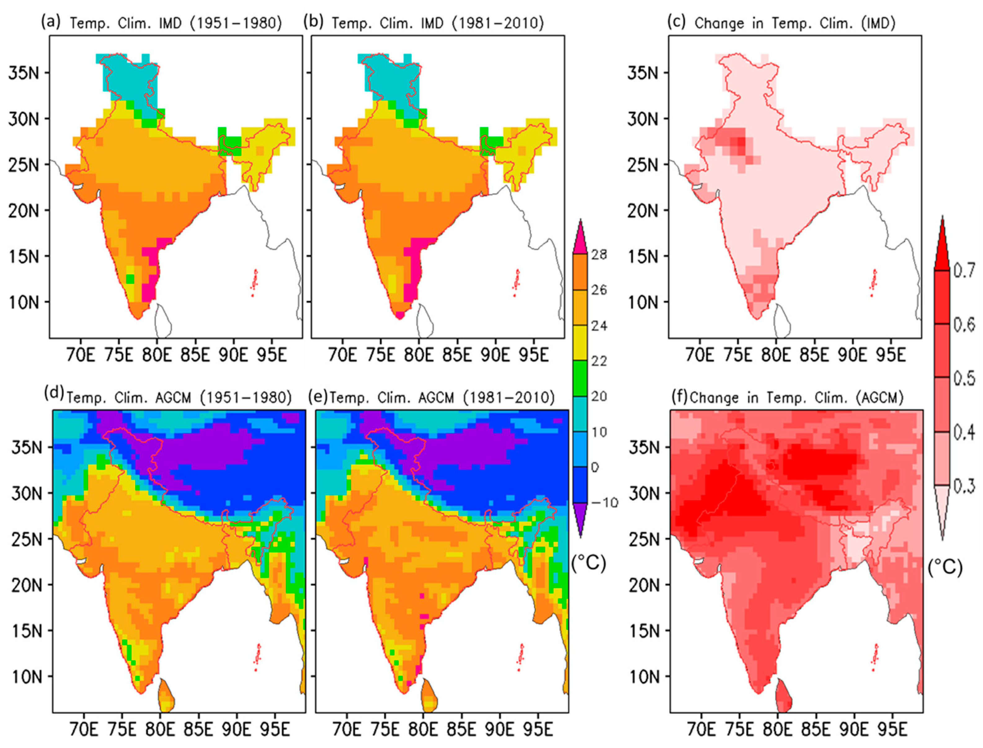
The spatial distribution of temperature climatology derived from the IMD observation and that from the AGCM ensemble mean for the periods 1951–1980 and 1981–2010 are presented in Figure 9. Both the observed and the model simulated results indicate that the mean surface temperatures over most of the Indian regions varies in the range of 24–28 °C. Few regions of north India along the Himalayan belt experience the lowest temperature of about or less than 0 °C, while few regions of south India shows higher temperatures of about or higher than 28 °C during 1981–2010.
The model successfully represented variation of temperature pattern over Indian region, but with slightly lower magnitudes compare to the observation, particularly few regions of north and south India, indicating a cold bias in the model for these regions. Overall, the model simulated mean surface temperature over most of Indian regions has a good agreement with the observation. The standard deviation of each individual ensemble climatology from their mean climatology is found in the range 0.5–0.15 °C (Figure 10). The comparison between the temperature climatologies during 1951–1980 and 1981–2010 indicates that the temperature is increased over entire region. Northwestern regions of India show maximum increase in temperature in recent climate period. Both model and observation show similar increased pattern of temperature (Figure 9c,f). The p-values from the Student’s t-test by assigning null hypothesis to no temperature change between the two periods at 95% significance level is found lower over most of the regions of India with exceptions over some regions of northern and southern India. So the temperature change over most of the Indian regions are significant although few regions show no temperature change. Overall, the increased temperature in the recent climate period is qualitatively well represented in model simulations with higher values by about 0.2–0.3 °C.

3.3.2. Annual Cycles and Frequency Distributions

Figure 11 represents the annual cycles and frequency distribution of the monthly mean temperatures over India during 1951–1980 and 1981–2010 from the AGCM model simulations and that of from the IMD observation. The results from the model simulations indicate that the monthly mean temperature over India varies from 15 °C during December–January to 29 °C in May. Observed mean temperature over India also shows similar pattern, but the magnitudes vary from ~17 °C during December–January to 30 °C in May. Overall, the model simulated monthly mean temperatures over India show a cold bias in both the climate periods. However, both model and observation show an increase of the mean temperature over India during July through March in recent climate (Figure 11c). Observed mean temperature during April–June does not changes considerably in both climate periods. The normal probability distribution functions from monthly mean temperatures indicate a shifting of about 3 °C at the peak temperatures between the model and observation. Model simulated results show that most of the months over India during 1951–1980 and 1981–2010 had temperature ~22 °C while observation shows the same had ~25 °C. We analyzed the frequency of monthly mean temperatures in 2 °C interval during two climate periods and found that the more months had mean temperature of 28–31 °C in recent climate period (Figure 11f), indicating an overall increase of mean temperature over India in recent climate period.

3.4. Climatology of Other Environmental Conditions

The climatology of precipitation indicated a decrease of precipitation amount in recent climate period. Previous studies (e.g., [11,14]) also observed negative precipitation trends over various regions of India. To understand the mechanism of decreased precipitation, we analyzed the vertical velocity (Omega), specific humidity, upper air temperature, cloud and relative humidity at 500 hPa during two climate periods and their changes in recent climate period (Figure 12). We find that the omega is higher in the recent climate period (i.e., 1981–2010) over Indian regions, implying relatively weaker upward motion of air compared to that during 1951–1980 (Figure 12c). Specific humidity and temperature at 500 hPa are increased in recent climate over almost entire Indian regions except western regions (specific humidity decreased) (Figure 12f,j). Cloud and relative humidity are also decreased in recent climate period over entire Indian regions (Figure 12l,o). All these implies that the decrease of relative humidity and cloud together with weaker vertical velocity could be the reason of decrease of precipitation over Indian region in recent climate period. Although an increase of specific humidity and temperature are noticed over most of the regions, but water vapor could saturate enough due to lower percentage of humidity. We further found that temperature is increased over entire regions of India in recent climate period. Multitudes of previous studies (e.g., [17,20,47,48,49]) also highlighted an increase of temperature trends over Indian regions. The reason could be associated with many factors such as increase of greenhouse gas concentrations in the air, land use changes, human activities. There are plenty of debate in this context and can be found in IPCC reports [1,2].

4. Discussion and Conclusions

This study presents the precipitation and temperature climatologies over India from 100 ensemble climate simulations by AGCM during recent past periods (1951–2010). We examined the usefulness of the AGCM climate simulation products to capture the precipitation and temperature climatologies and their distribution patterns over India. We found that the AGCM model captured the precipitation climatology reasonably well for all months except December and January with standard deviations below 1 mm/day with correlation coefficient above 0.6 during June–November, 1.5 mm/d with correlation 0.6 during December and in the range of 1–2 mm/day with correlation more than 0.7 in other months. The model reproduced the temperature distribution pattern well enough with correlation coefficients higher than 0.7, but with higher standard deviation. The EOF analysis indicated that the model captured various observed precipitation variabilities as described by the dominant EOFs.
We next discussed the precipitation and temperature change between two climate periods viz. 1951–1980 and 1981–2010. The results indicated that the precipitation and temperature climatology patterns in both climate periods were almost similar but their magnitudes were not same, indicating a possible influence of climate change. The precipitation amount over many regions of India are decreased in recent climate period i.e., 1981–2010 compared to that in past climate period i.e., 1951–1980. The reason of decreased precipitation could be attributed to a decrease of relative humidity and cloud together with weaker vertical velocity over Indian region in recent climate period. We further found an increase of temperature over entire regions of India in recent climate period.
We further investigated the annual cycle of the temperatures and precipitations over India during the two climate periods and their frequency distributions. We find that a decrease of the precipitation amounts over India in recent climate period for the months from June through October and an increase of precipitation amount for the months May and from November through January. The monthly mean temperature over India is increased during July through March in recent climate, while the mean temperature does not change notably during April–June. The frequency distributions of monthly precipitations indicate an overall decrease of precipitation amount and an overall increase of mean temperature in recent climate period.
These results are important to enhance the understanding of climate change over India from large ensemble historical experiment results. Although a number of previous studies have discussed the Indian climatology and our results also appeared to be consistent with previous studies, but the present study with large ensemble climate simulations would lead to overall confidence in climate change assessments in India. Moreover, most of the previous studies consider the monsoonal precipitation. Therefore, to reveal and better characterize climate change over India particularly the future projection of Indian climate, the present validation of the AGCM large ensemble climate simulation products over India may help to decide whether these ensembles to use for the uncertainty assessments in the context of climate risk management. So, we believe that our study based on the large ensemble simulation experiments would give an idea towards the assessment of the climate change impact in India. These datasets may be further analyzed through different methods e.g., periodograms to enhance the hidden cycles of precipitation and temperature over India.

Author Contributions

Conceptualization, S.N.; Formal analysis, S.N., T.T. and S.M.; Funding acquisition, T.T.; Investigation, S.N.; Methodology, S.N., T.T. and S.M.; Software, S.M.; Validation, S.N.; Visualization, S.M.; Writing—original draft, S.N.; Writing—review and editing, T.T. All authors have read and agreed to the published version of the manuscript.

Funding

This study was supported by the TOUGOU program (Grant Number JPMXD0717935498) and funded by the Ministry of Education, Culture, Sports, Science, and Technology, Government of Japan. This study was also supported by Grants-in-Aid for Scientific Research from the Japan Society for the Promotion of Science 18H01680, 20H00289, and 21H01591.

Institutional Review Board Statement

Not applicable.

Informed Consent Statement

Not applicable.

Data Availability Statement

The d4PDF data (the database for Policy Decision making for Future climate change) dataset supporting the conclusions of this article is obtained from the Data Integration and Analysis System (DIAS, http://search.diasjp.net/en/dataset, accessed on 10 February 2020). The precipitation and temperature observation dataset supporting the validation of this study is obtained from the Indian Meteorological Department (IMD, https://mausam.imd.gov.in/, accessed on 20 November 2016).

Acknowledgments

This study was supported by the TOUGOU program (Grant Number JPMXD0717935498) and funded by the Ministry of Education, Culture, Sports, Science, and Technology, Government of Japan. This study was also supported by Grants-in-Aid for Scientific Research from the Japan Society for the Promotion of Science 18H01680, 20H00289, and 21H01591. Japan Meteorological Agency (JMA) is acknowledged for providing Radar/Rain gauge—Analyzed Precipitation product.

Conflicts of Interest

The authors declare no conflict of interest.

References

  1. IPCC. Synthesis Report Summary for Policymakers 2014. Available online: https://www.ipcc.ch/pdf/assessment-report/ar5/syr/AR5_SYR_FINAL_SPM.pdf. (accessed on 19 December 2019).
  2. IPCC. Summary for policymakers. In Climate Change 2021: The Physical Science Basis. In Contribution of Working Group I to the Sixth Assessment Report of the Intergovernmental Panel on Climate Change; Masson-Delmotte, V., Zhai, P., Pirani, A., Connors, S.L., Péan, C., Berger, S., Caud, N., Chen, Y., Goldfarb, L., Gomis, M.I., et al., Eds.; Available online: https://www.ipcc.ch/report/ar6/wg1/downloads/report/IPCC_AR6_WGI_SPM_final.pdf (accessed on 10 January 2022).
  3. Takemi, T.; Okada, Y.; Ito, R.; Ishikawa, H.; Nakakita, E. Assessing the impacts of global warming on meteorological hazards and risks in Japan: Philosophy and achievements of the SOUSEI program. Hydrol. Res. Lett. 2016, 10, 119–125. [Google Scholar] [CrossRef] [Green Version]
  4. Akdi, Y.; Ünlü, K.D. Periodicity in precipitation and temperature for monthly data of Turkey. Theor. Appl. Climatol. 2021, 143, 957–968. [Google Scholar] [CrossRef]
  5. Liu, Y.; Roberts, M.C.; Sioshansi, R. A vector autoregression weather model for electricity supply and demand modeling. J. Mod. Power Syst. Clean Energy 2018, 6, 763–776. [Google Scholar] [CrossRef] [Green Version]
  6. Tektaş, M. Weather forecasting using ANFIS and ARIMA models. Environ. Res. Eng. Manag. 2010, 51, 5–10. [Google Scholar]
  7. Singh, A.; Kulkarni, M.A.; Mohanty, U.; Kar, S.; Robertson, A.W.; Mishra, G. Prediction of Indian summer monsoon rainfall (ISMR) using canonical correlation analysis of global circulation model products. Meteorol. Appl. 2012, 19, 179–188. [Google Scholar] [CrossRef] [Green Version]
  8. Shukla, R.P. The dominant intraseasonal mode of intraseasonal South Asian summer monsoon. J. Geophys. Res. Atmos. 2014, 119, 635–651. [Google Scholar] [CrossRef]
  9. Sharma, S.K.; Bhattacharya, S.; Garg, A. Vulnerability and Adaptation. In India’s Initial National Communication (NATCOM) to United Nations Framework Convention on Climate Change and the Forestry Sector; Ministry of Environment and Forests, Government of India: New Delhi, India, 2004; pp. 59–71. [Google Scholar]
  10. Nayak, S.; Mandal, M.; Maity, S. Performance evaluation of RegCM4 in simulating temperature and precipitation climatology over India. Theor. Appl. Climatol. 2019, 137, 1059–10751. [Google Scholar] [CrossRef]
  11. Kishore, P.; Jyothi, S.; Basha, G.; Rao, S.V.B.; Rajeevan, M.; Velicogna, I.; Sutterley, T.C. Precipitation climatology over India: Validation with observations and reanalysis datasets and spatial trends. Clim. Dyn. 2016, 46, 541–556. [Google Scholar] [CrossRef] [Green Version]
  12. Dey, P.; Mujumdar, P.P. On the uniformity of rainfall distribution over India. J. Hydrol. 2019, 578, 124017. [Google Scholar] [CrossRef]
  13. Goswami, B.N.; Venugopal, V.; Sengupta, D.; Madhusoodanan, M.S.; Xavier, P.K. Increasing trend of extreme rain events over India in a warming environment. Science 2006, 314, 1442–1445. [Google Scholar] [CrossRef] [Green Version]
  14. Dash, S.K.; Kulkarni, M.A.; Mohanty, U.C.; Prasad, K. Changes in the characteristics of rain events in India. J. Geophys. Res. 2009, 114, D10109. [Google Scholar] [CrossRef]
  15. Lacombe, G.; McCartney, M. Uncovering consistencies in Indian rainfall trends observed over the last half century. Clim. Change 2014, 123, 287–299. [Google Scholar] [CrossRef]
  16. Sinha Ray, K.C.; Srivastava, A.K. Is there any change in extreme events like droughts and heavy rainfall? Curr. Sci. 1999, 79, 155–158. [Google Scholar]
  17. Dash, S.K.; Jenamani, R.K.; Kalsi, S.R.; Panda, S.K. Some evidence of climate change in twentieth-century India. Clim. Change 2007, 85, 299–321. [Google Scholar] [CrossRef]
  18. Pattanaik, D.R.; Kumar, A. Prediction of summer monsoon rainfall over India using the NCEP climate forecast system. Clim. Dyn. 2010, 34, 557–572. [Google Scholar] [CrossRef]
  19. DelSole, T.; Shukla, J. Climate models produce skillful predictions of Indian summer monsoon rainfall. Geophys. Res. Lett. 2012, 39, 99–109. [Google Scholar] [CrossRef] [Green Version]
  20. Nayak, S.; Mandal, M. Impact of Land Use and Land Cover Change on Temperature Trends over Western India. Curr. Sci. 2012, 102, 1166–1173. [Google Scholar]
  21. Prakash, S.; Mitra, A.K.; Momin, I.M.; Rajagopal, E.N.; Basu, S.; Collins, M.; Ashok, K. Seasonal intercomparison of observational rainfall datasets over India during the southwest monsoon season. Int. J. Climatol. 2015, 35, 2326–2338. [Google Scholar] [CrossRef] [Green Version]
  22. Nayak, S.; Mandal, M.; Maity, S. Customization of regional climate model (RegCM4) over Indian region. Theor. Appl. Climatol. 2017, 127, 153–168. [Google Scholar] [CrossRef]
  23. Maity, S.; Mandal, M.; Nayak, S.; Bhatla, R. Performance of cumulus parameterization schemes in the simulation of Indian Summer Monsoon using RegCM4. Atmósfera 2017, 30, 287–309. [Google Scholar] [CrossRef] [Green Version]
  24. Maity, S.; Satyanarayana, A.N.V.; Mandal, M.; Nayak, S. Performance evaluation of land surface models and cumulus convection schemes in the simulation of Indian summer monsoon using a regional climate model. Atmos. Res. 2017, 197, 21–41. [Google Scholar] [CrossRef]
  25. Nayak, S.; Mandal, M.; Maity, S. RegCM4 simulation with AVHRR land use data towards temperature and precipitation climatology over Indian region. Atmos. Res. 2018, 214, 163–173. [Google Scholar] [CrossRef]
  26. Panda, A.; Sahu, N. Trend analysis of seasonal rainfall and temperature pattern in Kalahandi, Bolangir and Koraput districts of Odisha, India. Atmos. Sci. Lett. 2019, 20, e932. [Google Scholar] [CrossRef] [Green Version]
  27. Saini, A.; Sahu, N.; Kumar, P.; Nayak, S.; Duan, W.; Avtar, R.; Behera, S. Advanced Rainfall Trend Analysis of 117 Years over West Coast Plain and Hill Agro-Climatic Region of India. Atmosphere 2020, 11, 1225. [Google Scholar] [CrossRef]
  28. Bhatla, R.; Verma, S.; Ghosh, S.; Mall, R.K. Performance of regional climate model in simulating Indian summer monsoon over Indian homogeneous region. Theor. Appl. Climatol. 2020, 139, 1121–1135. [Google Scholar] [CrossRef]
  29. Kumar, D.; Dimri, A.P. Sensitivity of convective and land surface parameterization in the simulation of contrasting monsoons over CORDEX-South Asia domain using RegCM-4.4. 5.5. Theor. Appl. Climatol. 2020, 139, 297–322. [Google Scholar] [CrossRef]
  30. Nayak, S.; Mandal, M.; Maity, S. Assessing the impact of Land-use and Land-cover changes on the climate over India using a Regional Climate Model (RegCM4). Clim. Res. 2021, 85, 1–20. [Google Scholar] [CrossRef]
  31. Maity, S.; Nayak, S.; Singh, K.S.; Nayak, H.P.; Dutta, S. Impact of Soil Moisture Initialization in the Simulation of Indian Summer Monsoon Using RegCM4. Atmosphere 2021, 12, 1148. [Google Scholar] [CrossRef]
  32. Maity, S.; Nayak, S.; Nayak, H.P.; Bhatla, R. Comprehensive assessment of RegCM4 towards interannual variability of Indian Summer Monsoon using multi-year simulations. Theor. Appl. Climatol. 2022, 148, 1–26. [Google Scholar] [CrossRef]
  33. Nayak, S.; Takemi, T. Assessing the impact of climate change on temperature and precipitation over India. In Wadi Flash Floods: Challenges and Advanced Approaches for Disaster Risk Reduction; Sumi, T., Kantoush, S., Saber, M., Eds.; Springer: Singapore, 2022; pp. 121–142. [Google Scholar] [CrossRef]
  34. Bal, P.K.; Ramachandran, A.; Palanivelu, K.; Thirumurugan, P.; Geetha, R.; Bhaskaran, B. Climate change projections over India by a downscaling approach using PRECIS. Asia-Pac. J. Atmos. Sci. 2016, 52, 353–369. [Google Scholar] [CrossRef]
  35. Hawkins, E.; Sutton, R. The potential to narrow uncertainty in regional climate predictions. Bull. Am. Meteorol. Soc. 2009, 90, 1095–1108. [Google Scholar] [CrossRef] [Green Version]
  36. Wilks, D.S.; Wilby, R.L. The weather generation game: A review of stochastic weather models. Prog. Phys. Geogr. 1999, 23, 329–357. [Google Scholar] [CrossRef]
  37. Fowler, H.J.; Blenkinsop, S.; Tebaldi, C. Linking climate change modelling to impacts studies: Recent advances in downscaling techniques for hydrological modelling. Int. J. Climatol. J. R. Meteorol. Soc. 2007, 27, 1547–1578. [Google Scholar] [CrossRef]
  38. Croce, P.; Formichi, P.; Landi, F. Enhancing the output of climate models: A weather generator for climate change impact studies. Atmosphere 2021, 12, 1074. [Google Scholar] [CrossRef]
  39. Chaturvedi, R.K.; Joshi, J.; Jayaraman, M.; Bala, G.; Ravindranath, N.H. Multi-model climate change projections for India under representative concentration pathways. Curr. Sci. 2012, 103, 791–802. [Google Scholar]
  40. Akhter, J.; Das, L.; Deb, A. CMIP5 ensemble-based spatial rainfall projection over homogeneous zones of India. Clim. Dyn. 2017, 49, 1885–1916. [Google Scholar] [CrossRef]
  41. Mizuta, R.; Murata, A.; Ishii, M.; Shiogama, H.; Hibino, K.; Mori, N.; Arakawa, O.; Kawase, H.; Mori, M.; Okada, Y.; et al. Over 5000 years of ensemble future climate simulations by 60-km global and 20-km regional atmospheric models. Bull. Am. Meteorol. Soc. 2017, 98, 1383–1398. [Google Scholar] [CrossRef]
  42. Iizumi, T.; Shiogama, H.; Imada, Y.; Hanasaki, N.; Takikawa, H.; Nishimori, M. Crop production losses associated with anthropogenic climate change for 1981–2010 compared with preindustrial levels. Int. J. Climatol. 2018, 38, 5405–5417. [Google Scholar] [CrossRef] [Green Version]
  43. Hatsuzuka, D.; Sato, T. Future Changes in Monthly Extreme Precipitation in Japan Using Large-Ensemble Regional Climate Simulations. J. Hydrometeorol. 2019, 20, 563–574. [Google Scholar] [CrossRef]
  44. Perkins, S.E.; Pitman, A.J.; Holbrook, N.J.; McAneney, J. Evaluation of the AR4 climate models’ simulated daily maximum temperature, minimum temperature, and precipitation over Australia using probability density functions. J. Clim. 2007, 20, 4356–4376. [Google Scholar] [CrossRef]
  45. Taylor, K.E. Summarizing multiple aspects of model performance in a single diagram. J. Geophys. Res. Atmos. 2001, 106, 7183–7192. [Google Scholar] [CrossRef]
  46. North, G.R.; Bell, T.L.; Cahalan, R.F.; Moeng, F.J. Sampling errors in the estimation of empirical orthogonal functions. Mon. Weather Rev. 1982, 110, 699–706. [Google Scholar] [CrossRef]
  47. Nayak, S.; Mandal, M. Impact of land use and land cover changes on temperature trends over India. Land Use Policy 2019, 89, 104238. [Google Scholar] [CrossRef]
  48. Nayak, S.; Maity, S.; Singh, K.S.; Nayak, H.P.; Dutta, S. Influence of the Changes in Land-Use and Land Cover on Temperature over Northern and North-Eastern India. Land 2021, 10, 52. [Google Scholar] [CrossRef]
  49. Nayak, S.; Maity, S.; Sahu, N.; Saini, A.; Singh, K.S.; Nayak, H.P.; Dutta, S. Application of “Observation Minus Reanalysis” Method towards LULC Change Impact over Southern India. ISPRS Int. J. Geo. Inf. 2022, 11, 94. [Google Scholar] [CrossRef]
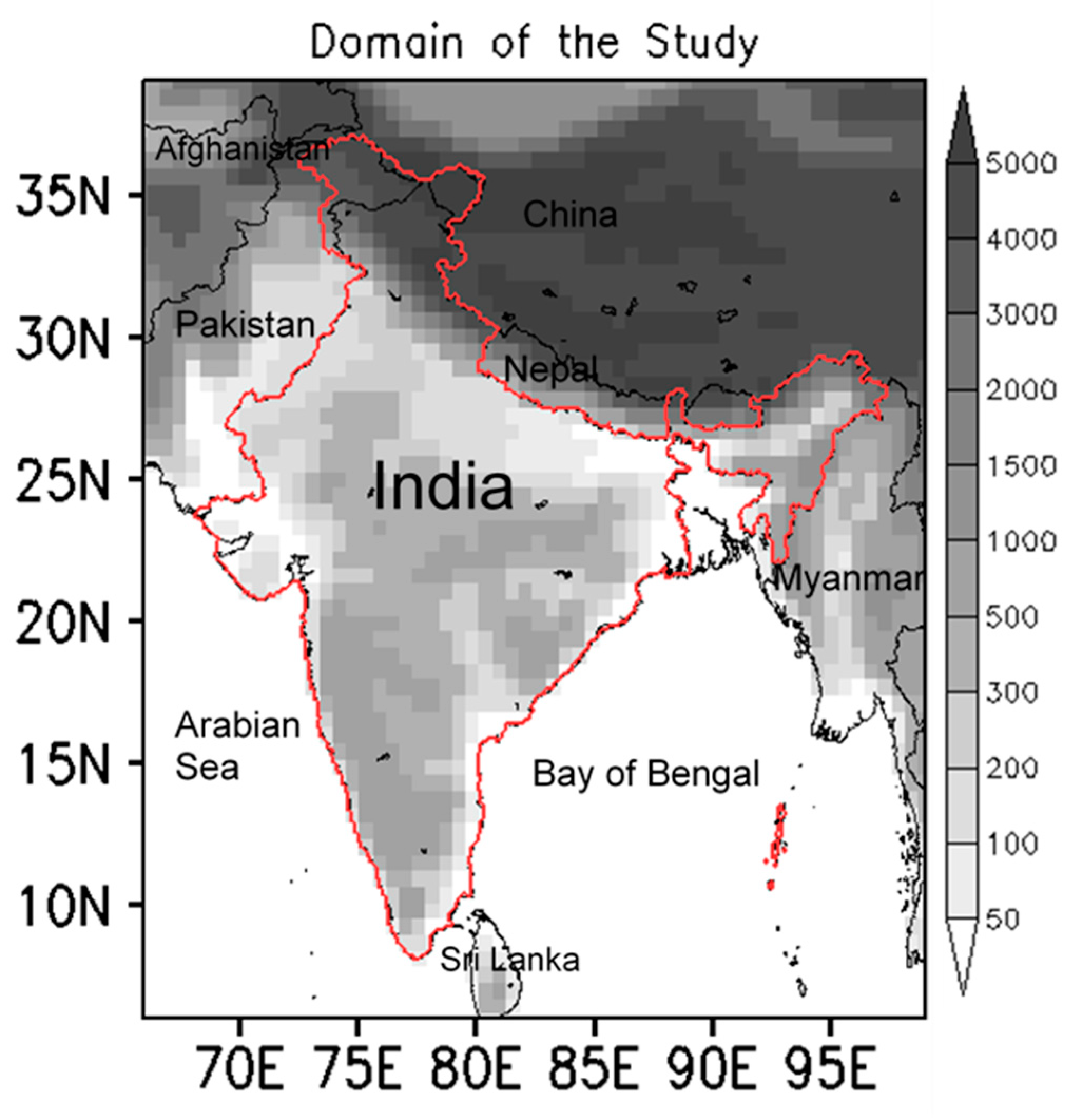
Figure 1. Study region with topography (unit: m). The red colour marked map indicates India.
Atmosphere 13 00671 g001
Figure 2. Taylor diagram showing correlations coefficients, standard deviations and RMSEs between AGCM simulations and IMD observation of precipitation for the two climate periods (a) 1951–1980 and (b) 1981–2010. Dark color marks correspond to the results for ensemble mean and light color marks correspond to each individual member.
Atmosphere 13 00671 g002
Figure 3. Taylor diagram showing correlations coefficients, standard deviations and RMSEs between AGCM simulations and IMD observation of temperature for the two climate periods (a) 1951–1980 and (b) 1981–2010. Dark color marks correspond to the results for ensemble mean and light color marks correspond to each individual member.
Atmosphere 13 00671 g003
Figure 4. First three EOFs and their corresponding PCs of the precipitation for the period 1951–1980 from (af) AGCM ensemble and (gl) IMD observation.
Atmosphere 13 00671 g004
Figure 5. First three EOFs and their corresponding PCs of the temperature for the period 1981–2010 from (af) AGCM ensemble and (gl) IMD observation.
Atmosphere 13 00671 g005
Figure 6. Precipitation climatology in two climate periods from (a,b) AGCM ensemble and (d,e) IMD observation. Change in precipitation climatology from (c) IMD and (f) AGCM.
Atmosphere 13 00671 g006
Figure 7. Standard deviation (STD) of the precipitation climatologies derived from all ensemble members in two climate periods (a) 1951–1980 and (b) 1981–2010.
Atmosphere 13 00671 g007
Figure 8. (a,b) Annual cycle, and (d,e) PDFs of precipitation. Change in (c) precipitation and (f) frequency in two climate periods. Thin lines in (ad) correspond to the results for each individual member.
Atmosphere 13 00671 g008
Figure 9. Temperature climatology in two climate periods from (a,b) AGCM ensemble and (d,e) IMD observation. Change in temperature climatology from (c) IMD and (f) AGCM.
Atmosphere 13 00671 g009
Figure 10. Standard deviation of the temperature climatologies derived from all ensemble members in two climate periods (a) 1951–1980 and (b) 1981–2010.
Atmosphere 13 00671 g010
Figure 11. (a,b) Annual cycle, and (d,e) PDFs of temperature. Change in (c) temperature and (f) frequency in two climate periods. Thin lines in (a,d) correspond to the results for each individual member.
Atmosphere 13 00671 g011
Figure 12. Climatogies in two climate periods at 500 hPa and change in (ac) omega, (df) specific humidity, (g,h) temperature, (ik) Cloud cover, and (lo) relative humidity. 1st panel corresponds to the results for the period 1951–1980, 2nd panel corresponds to the results for the period 1981–2010, and 3rd panel corresponds to their change in recent period.
Atmosphere 13 00671 g012
Publisher’s Note: MDPI stays neutral with regard to jurisdictional claims in published maps and institutional affiliations.