Abstract
Four typical double-moment cloud microphysical schemes (Milbrandt, Morrison, NSSL and WDM6) in WRF (Weather Research and Forecasting) are used to investigate the impact of the different schemes on the simulation of a straight squall line evolving into a bow-shaped one in East China on 15 April 2016. Although simulations with Milbrandt, Morrison and WDM6 schemes can produce bow-shaped squall lines, only the WDM6 scheme can simulate the evolution process of the straight squall line to a bow-shaped one well. The simulation results with the NSSL scheme produce a broken straight squall line. The possible reason is that the range and intensity of cold pools and the rear inflows are different among the four schemes when the observed squall line evolves into a standard bow-shaped squall line. The mixing ratio and number concentration of rain water with the WDM6 scheme is largest in strong convective areas, and the cold pool and rear inflow are also strongest among the four schemes. Compared with the WDM6 scheme, the mixing ratio and number concentration of rain water are less with the Milbrandt and Morrison schemes. Also, the cold pool and rear inflow with the Milbrandt scheme are weaker than for the WDM6 scheme but stronger than those with the Morrison scheme. The rainwater mixing ratio is very low and no obvious cold pool and rear inflow exist with the NSSL scheme.
1. Introduction
Squall lines are one type of mesoscale convective systems (MCSs), which consist of a series of active convective storms, at scales greater than 100 km [1]. When a squall line passes by, it often causes severe disasters, such as thunderstorms, heavy rain, strong winds, hail, and tornadoes. Bow-shaped squall lines are usually associated with downbursts and swathes of damaging winds [2], which are more likely to produce severe weather than straight squall lines [3]. Due to the low spatial and temporal resolution of conventional meteorological observations, it is difficult to capture the evolution characteristics of squall lines, and it is even more difficult to determine whether the squall line can evolve into a bow-shaped squall line or not. High resolution simulation provides an important way to study squall lines, but accurate prediction of the process by which a straight squall line evolves into a bow-shaped one is still full of challenges due to large uncertainties in the initial conditions, and in model physics process parameterization schemes.
Doppler radar is an important meteorological observing platform capable of providing sufficient temporal and spatial resolution data to capture storm-scale features [4]. Assimilating Doppler radar data (reflectivity and radial velocity) into the numerical model can produce a more accurate initial condition, and thus reduce forecast errors [5,6,7,8]. The improved simulation results can help us to analyze and diagnose uncertainties in model physics parameterization schemes. Furthermore, the spatial distribution characteristics of radial velocity can provide some information about the tangential wind component [9,10]. In addition to radial velocity, assimilation of the spatial distribution characteristics of radial velocity should further improve the model wind field [11,12].
In addition to the initial condition, physical processes have a large impact on forecast accuracy. The Intergovernmental Panel on Climate Change (IPCC) clearly points out that cloud microphysical process and its feedback mechanism are the biggest factors leading to uncertainty in numerical weather prediction (NWP) [13]. At present, there are still large uncertainties in the parameterization scheme of cloud microphysical processes in both weather and climate models [14]. Most cloud microphysics parameterization (MP) use bulk schemes that predict hydrometeors mass mixing ratios and/or number concentrations by assuming a size distribution, such as gamma distribution or empirical exponential distribution [15,16,17,18]. Bulk MP schemes can be further divided into single-moment methods and double-moment methods. Single-moment bulk MP schemes only predict the mixing ratios of hydrometeors [19], the intercept of the spectrum distribution is assumed to be constant, and the evolution of the particle spectrum is determined by slope change. Double-moment bulk MP schemes predict both the mixing ratio of the hydrometeors and their number concentrations [20,21], and the evolution of particle spectrum is determined by both slope and intercept. Thus, the description of the cloud microphysical process in double-moment bulk MP schemes should be more reasonable in theory.
Many studies [22,23,24,25] have shown double-moment MP schemes have better performance in terms of squall lines simulation. For example, Morrison et al. (2009) [23] compared the impact of a single-moment with a double-moment MP scheme on the development of trailing stratiform precipitation in a simulated squall line using the WRF model, and found that the double-moment MP scheme reduced the rain evaporation rate in the stratiform area with a wider range of stratiform area. Hong et al. (2010) [24] showed that the WDM6 double-moment scheme could effectively improve the simulation results of convective characteristics of a bow-shaped squall line. Huang et al. (2017) [25] used different MP schemes in the WRF model to simulate a squall line in East China and showed that double-moment MP schemes performed better than single-moment MP schemes, especially the WDM6 scheme. The above studies mainly focus on the squall lines occurring under relatively large CAPE, while the impact of the MP schemes on simulation of squall lines occurring under relatively stable conditions are relatively few. In addition, only a few studies have focused on the impact of different double-moment MP schemes on the process of a straight squall line evolving into a bow-shaped squall line, especially happening in an environmental condition with a low CAPE. Considering that dynamic and thermodynamic environments have a possible influence on cloud microphysics processes, it is necessary to further study the differences of a simulated bow-shaped squall line with different double-moment MP schemes in different background synoptic environments and find out the main drivers of these differences.
In this study, we performed a set of experiments with four different double-moment MP schemes (i.e., Milbrandt, Morrison, NSSL and WDM6) in WRF to investigate their capabilities to reproduce a bow-shaped squall line as happened under a low CAPE and an intense vertical wind shear in East China on 15 April 2016. The underlying reasons for discrepancies of the simulations among different schemes were explored, based on the dynamic, thermal structure and hydrometeors distribution characteristics. To reduce the uncertainties in initial conditions and improve the simulations, radar reflectivity and radar radial velocity data and the spatial distribution characteristics of the radial velocity were assimilated. The implications and limitations of our conclusions are also discussed. This paper is organized as follows: Section 2 briefly introduces the 15 April 2016 squall line. Section 3 describes the numerical model, data assimilation method, and experimental setup and then briefly introduces the four double-moment microphysical schemes used in this study. Simulation results are verified and analyzed in Section 4. A summary is provided in Section 5. A discussion is provided in Section 6.
2. Case Overview
A mesoscale convective system developed from scattered thunderstorms in Hunan Province (location is shown in Figure 1a, similarly hereinafter) around 1700 UTC on 15 April 2016. The storms moved eastward rapidly and gradually organized into a squall line in the western Jiangxi Province at 2000 UTC on 15 April. The squall line affected Jiangxi from 2000 UTC on 15 April to 0200 UTC on 16 April with short-term strong winds and short-duration heavy rains (Figure 1b, red dashed line represents the approximate position of the squall line at the corresponding time, determined by the position of the strongest radar composite reflectivity, which was obtained from the radar base data of the nearest 6 min). Based on observations at the regional automatic meteorological stations of China, eight stations showed short-term strong winds of more than 24.5 m·s−1, and the largest of up to 33.8 m·s−1. A total of 27 cities and counties experienced short-time heavy rainfall (≥20 mm in 1 h), and the heaviest was up to 46.2 mm in 1 h.
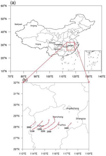
Figure 1.
(a) Locations of some provinces in China which are discussed in this paper (Jiangxi, Hunan, Xinjiang, Sichuan, Chongqing, Guizhou, Xizang), the red box is the area of b; (b) Locations of five radars (Nanchang, Yichun, Jingdezheng, Shangrao, and Fuzhou) used in this study. (Red dashed line represents the path of the squall line obtained from the radar composite reflectivity from 2000 UTC to 2400 UTC on 15 April 2016).
2.1. Environmental Conditions
To explore the environmental conditions before the squall line happened, the six-hourly National Centers for Environmental Prediction (NCEP) reanalysis dataset, with a resolution of 1° × 1°, was used. As shown in Figure 2a, there was a ridge of high pressure in the balk hash lake area, continuous cold air along the west of Xinjiang province entered into China from the front of the ridge at 500 hPa at 1200 UTC on 15 April 2016. A low trough was located in a low latitude plateau region, west of Sichuan province. The southwest jet stream flowed over Hunan, northern and central Jiangxi. In addition, the temperature trough lagged behind the height trough, and the strong baroclinic effect made the low trough of upper air move eastward and continuously develop.
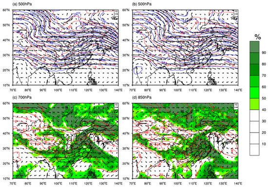
Figure 2.
500 hPa geopotential height (blue solid lines, units: dagpm) and wind field (vectors, units: m·s−1) and temperature (red solid lines, units: °C) at 1200 UTC (a) and at 1800 UTC, (b) and wind field (vectors, units: m·s−1), temperature (red solid lines, units: °C) and relative humidity (shaded, units: %) at 700 hPa (c) and 850 hPa (d) at 1800 UTC on 15 April 2016.
By 1800 UTC (Figure 2b), the low trough at 500 hPa had moved eastward to Chongqing and the east of Guizhou. The cold air behind the trough moved southward and converged with the warm and wet southwest current over Hunan. At 700 hPa and 850 hPa (Figure 2c,d), Hunan, central and northern Jiangxi, were all located in the warm and wet southwest air, where relative humidity was 60–80% at 700 hPa, more than 80% at 850 hPa in most areas, and more than 90% at 850 hPa in some areas. The warm and wet southwest current provided sufficient water vapor for the occurrence of the squall line, and the water vapor in the lower levels was more abundant than that in the upper levels. At 850 hPa, there were northwest to southwest wind shears in Hunan.
Convective available potential energy (CAPE) at Huanghua station in Hunan Province was 329.3 J·kg−1, and 0 J·kg−1 at Nanchang station in Jiangxi Province (Figure 3), which was below the average value for the midlatitude squall lines [26]. Moreover, the ground heating effect was very small and the CAPE would not increase, because the squall line appeared at night. Therefore, the CAPE was not conducive to the formation of bow-shaped squall lines. The difference between the dewpoint temperature and temperature below 3 km were small at the two stations but significantly increased above 3 km, indicating that abundant water vapor existed in the middle and lower levels at this time, which promoted the formation of bow echoes in the warm season under the background of weak forcing [27,28]. In addition, veering winds within the 0–3 km layers were observed at two stations with strong vertical wind shears of 19 m·s−1 and 17 m·s−1, respectively. Therefore, the environmental conditions differed from typical bow-shaped squall lines [29] with a low CAPE and an intense vertical wind shear, which are more common for squall lines happening in south China [2].
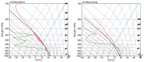
Figure 3.
T-lnP chart at Huanghua (a) and Nanchang (b) radiosonde station at 1200 UTC on 15 April 2016 (the green line represents dewpoint profile, the black line represents the lifting curve, the red line represents temperature profile).
2.2. Radar Composite Reflectivity
As shown in the mosaic of composite radar reflectivity, based on five SA-band Doppler radars (their locations are shown in Figure 1b), a linear convection system, with an orientation in the northeast–southwest direction, moved from Hunan to Jiangxi Province at 2000 UTC April 15 (Figure 4a). The horizontal scale of the convective line just reached the minimum scale of 100 km for a squall line, and the stratiform area at the back of the line was narrow. Two strong isolate convective cells existed in the northeast of the convective line, and merged with the line when moving eastward. By 2100 UTC (Figure 4b), a clear squall line, with northeast–southwest direction appeared in the east of Jiangxi Province with the strongest radar echo over 55 dBz. After that, the straight squall line gradually evolved into a bow-shaped squall line, with central intensity above 55 dBz (figure not shown). By 2230 UTC (Figure 4c), the squall line became a standard bow-shaped squall line, accompanied by a broad stratiform area and a bounded weak echo area between the convection and stratiform areas. After 2230 UTC, the squall line continued to move eastward, and the horizontal scale and width of the strong bow-shaped convection line gradually became shorter and narrower (Figure 4d,e). The squall line started to dissipate around 0030 UTC on 16 April 2016 (figure not shown) and completely weakened into a stratiform area at 0100 UTC (Figure 4f).
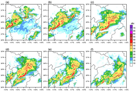
Figure 4.
Evolution of radar composite reflectivity (shaded, units: dBz) at 2000 UTC, (a) 100 UTC, (b) 2230 UTC, (c) 2300 UTC, (d) 15 April 2016 and 0000 UTC, (e) 0100 UTC, (f) 16 April 2016.
3. Methodology and Data
3.1. Introduction to Observation Operator for Radar Radial Velocity
In this paper, we adopted the radar radial velocity observation operator based on IVAP method [10] with the GSI Assimilation System to assimilate both the radial component of the velocity and the spatial distribution information of radial velocity. The calculation steps are as follows:
The conventional observation operator for Doppler radar radial velocity, as in GSI, is defined by:
where (u, v, w) are model wind components in the Cartesian coordinates of (x, y, z), θ is the azimuth of the radar observation, φ is the radar elevation angle, and Vr is the radar radial velocity. Since the control variable of GSI does not contain the vertical velocity w, the vertical term is ignored in the observation operator of radial velocity in GSI, namely:
If we consider a fixed region, both in the radar observation and model spaces, and regard it as Ω, we can obtain two spatial distribution characteristics of radial velocity by multiplying sinθ or cosθ on both sides of Equation (2) and summing within the given area Ω:
If we denote the averaged wind within Ω by , then Equation (3) can be expressed as:
The area-averaged wind can be calculated using the equation . For example, , N is the total number of the grid points within Ω. Dividing two sides of Equation (4) respectively by or , we get:
The left sides of Equation (5) are regarded as the observation spaces, the right sides of Equation (5) are defined as the analysis spaces, as follows:
Y1 and Y2 are regarded as new observations:
Equation (7) is used in this paper (referred to as IVAP observation operator hereafter) instead of Equation (2).
3.2. Introduction to the Cloud Analysis Method for Assimilating Reflectivity
Cloud analysis can incorporate cloud reports from surface observations, geostationary satellite infrared, visible imagery, radar reflectivity data and so on, to construct three-dimensional cloud cover, cloud water and ice mixing ratios, cloud and precipitate types, icing severity index, and snow, rain, graupel mixing ratios. Then, cloud-base, cloud-top, and cloud ceiling can be derived.
We used the cloud analysis method [6,30] within the GSI Assimilation System to assimilate radar reflectivity. The detailed process is shown in Figure 5. The ARPS [31] or RUC [32] scheme can be used to calculate the mixing ratios of cloud water and ice. The KRY [33], Lin [34] or Thompson [35] scheme can retrieve the mixing ratios of snow, rain, and graupel using radar reflectivity. The ARPS scheme (assuming that the vertical change of the temperature in-cloud is a wet adiabatic process) or RUC scheme (assuming that the vertical change of the temperature inside the cloud is a non-adiabatic process) can adjust the temperature in-cloud. The ARPS scheme or RUC scheme can adjust the water vapor in-cloud. Through sensitivity experiments, the following combination of different schemes can produce the best simulation for this squall line: the RUC scheme was used to calculate the mixing ratios of cloud water and ice, the Thompson scheme was selected to calculate the mixing ratios of snow, rain, and graupel, the ARPS scheme was used to adjust the in-cloud temperature, and the RUC scheme was chosen to adjust the in-cloud water vapor.
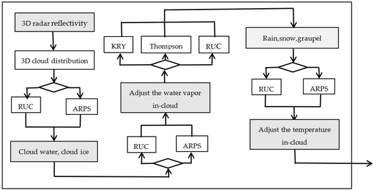
Figure 5.
Flow diagram of the cloud analysis method for assimilating reflectivity.
3.3. Model Configuration and Input Data
The data used included radiosonde observations, the six-hourly 1° × 1° NCEP reanalysis dataset, and five SA-band Doppler radars observations (Figure 1b) in Jiangxi Province, China.
Three two-way interactive nested domains were set for the WRF (Version 3.9.1) [36] model (Figure 6). The domains have 50 vertical layers with the model top at 50 hPa, and 301 × 301, 391 × 397, 601 × 466 grid points from outer domain to inner domain with horizontal grid point spacing of 9, 3, 1 km, respectively. The model starts at 1800 UTC 15 April 2016 with the initial and boundary conditions provided by the WRF Preprocessing System (WPS) initialization module by interpolating the 6-hourly 1° × 1° NCEP reanalysis dataset to the model grid points. Firstly, radar radial velocity data were assimilated by the GSI-3DVar (Version 3.4) with the IVAP observation operator and radar reflectivity data were assimilated by the cloud analysis method at 1800 UTC 15 April without cycling process. And then sensitivity tests were conducted by forecasts with four different double-moment MP schemes from 1800 UTC to 2400 UTC 15 April with a time step of 30 s. Results were provided every 30 min. The simulation results of a 1 km domain are analyzed in this paper. Some key physical parameterization schemes include the rapid radiative transfer model (RRTM) [37] for longwave radiation, the Dudhia [38] for shortwave radiation, the Yonsei State University (YSU) scheme [39] for planetary boundary layer processes, the Noah land surface scheme [40], the revised Monin-Obukhov mixed-layer scheme [41], and the Kain-Fritsch cumulus scheme [42] for the 9 km domain (no cumulus parameterization scheme was used for 3 and 1 km domains).
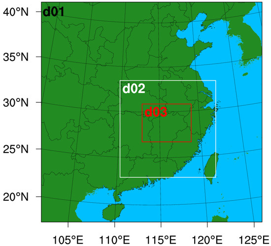
Figure 6.
Model domain coverage for the 15 April 2016 case (d01, d02, and d03 represent. the outer, middle and inner domains at 9 km, 3 km, and 1 km horizontal resolutions respectively).
In four sensitivity tests, the initial field and boundary conditions and physical parameterization schemes settings were the same, except for the MP schemes. Four typical double-moment MP schemes which are widely used in WRF were selected: WDM6 [18], Morrison 2-mom [23], Milbrandt-Yau 2-mom [43], and (National Severe Storms Laboratory) NSSL 2-mom [44] MP scheme. These specific double-moment MP schemes were chosen because they have had relatively good performances in previous studies [45,46,47,48]. The four MP schemes predict raindrop number concentration. In other words, they are double-moment for raindrops. There are noticeable differences among them. For example, the WDM6 scheme is based on the single-moment WSM6 scheme, the two-moment scheme is adopted to deal with the warm cloud precipitation process, and for all ice particles the single-moment is used. The microphysical process adds the numerical concentration prediction of cloud water, rain water and cloud condensation nuclei. The Morrison 2-mom is double-moment for all ice particles, but single-moment for cloud water. In this scheme, the shape of all particles is assumed to be spherical, the distribution of cloud droplets and raindrops follow Gamma function, and the distribution of rain, snow, graupel and ice particles adopt exponential function. The Milbrandt 2-mom scheme is double-moment for all liquid drops and ice particles, separates graupel and hail from each other and exists simultaneously as rimed ice particles, does not consider aerosol number concentration in the drop activation process, and predicts the number of nucleated droplets using a hardwired method [24]. The NSSL 2-mom is also double-moment for all liquid drops and ice particles, but this scheme predicts graupel as the only rimed ice particle. The WDM6 and Morrison 2-mom schemes can choose hail or graupel as required, we select graupel as the rimed ice particle in our study.
4. Results
4.1. Verification
In this paper, high resolution radar reflectivity observation data were used to verify the simulation results. The simulated and observed radar composite reflectivity at 2130 UTC, 2200 UTC, 2230 UTC 15 April 2016 are depicted in Figure 7, Figure 8 and Figure 9. It can be seen that the process of the straight squall line evolving into a bow-shaped squall line with the WDM6 scheme is similar to the observations, especially the strong convective line. However, the location and intensity of the strong convective area are slightly different from the observations, and the simulated stratiform area is too small. On the contrary, the simulated radar composite reflectivity with the Morrison, Milbrandt and NSSL schemes are different from the observations. Although the squall line with the Milbrandt scheme also evolves into a bow-shaped squall line, the bow-shaped structure differs significantly from the observations, with a loose and small strong convection area, and no obvious stratiform area. The structure of the strong convective area with the Morrison scheme is looser than with the Milbrandt scheme, with a larger difference from the observations. The strong convective area simulated by NSSL is discontinuous, and the strong convective line does not evolve into a bow-shaped structure, but a broken northeast–southwest convective line, and moves eastward. Among the four double-moment MP schemes, only the WDM6 scheme simulates the evolution process of the straight squall line into a bow-shaped one well.
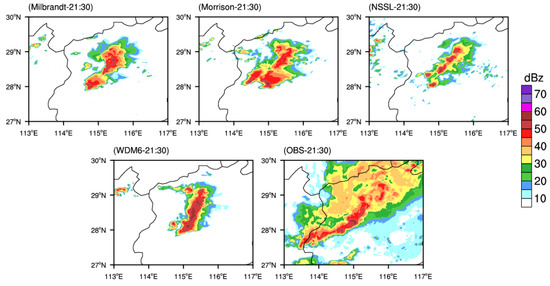
Figure 7.
The observed and simulated radar composite reflectivity with different double−moment. MP schemes at 2130 UTC 15 April 2016 (shaded, units: dBz).
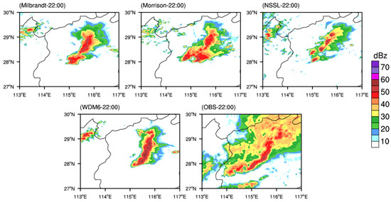
Figure 8.
Same as Figure 7 but at 2200 UTC.
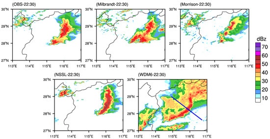
Figure 9.
Same as Figure 7 but at 2230 UTC. The blue line is the section position mentioned later.
Figure 10 shows the vertical cross section of the simulated and observed radar reflectivity across the blue line in Figure 9 at 2230 UTC 15 April 2016. The observed radar reflectivity top height is about 400 hPa, the largest radar reflectivity is up to more than 50 dBz, and the stratiform area is wide. The WDM6 simulates the structure of the strong convective area well, and reproduces the top height and strength of the strong convective area. But the simulated convective area is wider, and the range of the stratiform area is much smaller. The Morrison, and Milbrandt schemes also simulate strong convective areas, but the strength of the convective areas is weaker, and also no obvious stratiform area appears. The NSSL scheme does not generate a strong convective area with radar reflectivity larger than 35 dBz, and the simulation result is worst. In conclusion, compared with the other three schemes, the location and intensity of the strong convective area simulated by the WDM6 scheme are most consistent with observations.
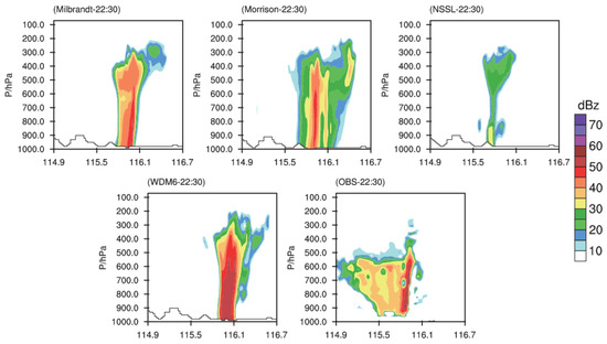
Figure 10.
The vertical cross section of observed and simulated radar reflectivity across the blue line in Figure 9 at 2230 UTC 15 April 2016 (shaded, units: dBz).
In order to quantitatively evaluate the simulation results, the threat scores (TS) and the neighborhood-based fractions skill score (FSS) are used to measure forecast skill.
TS is defined as:
where F gives the number of the events that are forecast, O gives the number of events that happened, C gives the number of those events that are correctly forecast.
FSS is defined by the formation:
where Pf and Po are the forecast and observed fractional coverages of a given adjacent area by reflectivity exceeding a given threshold value, and N is the number of grid points in the verification domain. We chose a square as the neighborhood region which contains 15 × 15 grids.
Figure 11 shows the TS and FSS for predicted reflectivity with thresholds of 40 dBz with four different double-moment MP schemes. The Milbrandt, Morrison, and WDM6 schemes have the highest TS and FSS at 2200 UTC, while the NSSL scheme gets the highest TS and FSS at 2130 UTC. In particular, the WDM6 scheme gives the consistently highest scores at all three times, followed by the Milbrandt and Morrison schemes. The NSSL scheme gets the lowest, and its TS and FSS values decrease rapidly as the integration time goes by, indicating that the NSSL scheme has a relatively poor performance in simulating the intensity and location of the squall line, especially at the mature stage when the observed squall line evolves into a bow-shaped squall line. The TS values of the Milbrandt and Morrison schemes maintain their value above 0.2 at all times, the FSS values of the Milbrandt and Morrison schemes maintain their value approximately equal to 0.5 at all times. The TS values of the WDM6 scheme are larger than 0.3 at three times with an average up to 0.343, the FSS values of the WDM6 scheme are larger than 0.5 at three times with the largest up to 0.65, which further indicates that this scheme has the best capability of simulating the location and the intensity of the strong convective area among the four schemes.
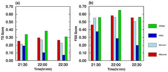
Figure 11.
(a) Threat scores and (b) Fractions Skill scores of predicted reflectivity for the 40 dBz threshold value with four double-moment MP schemes from 2130 UTC to 2230 UTC 15 April 2016.
In general, we find that all four double-moment MP schemes do not capture the stratiform area well enough. So, we focused on the strong convective region to judge the impact of the four double-moment MP schemes on simulation and explore the underlying reasons. In the following analyses we focus on the dynamic, thermal structure and hydrometeors distribution characteristics of the simulated strong convective region in squall lines at 2230 UTC, when the squall line evolved into the bow-shaped squall line.
4.2. Dynamic Characteristics
One main reason that a squall line evolves into a bow-shaped structure is the strong rear inflow jet existing in the middle and lower tropo-spheres [29]. The simulated 700 hPa horizontal storm-relative wind fields (the horizontal wind field minus the moving velocity of the squall line) with four different double-moment MP schemes at 2230 UTC are shown in Figure 12. The Milbrandt scheme (Figure 12a) shows southwest winds at the back of the strong convective area, and a rear inflow jet at the back of the squall line, which is favorable for the squall line to evolve into a bow-shaped structure. The Morrison scheme (Figure 12b) shows west winds at the back of the strong convective area, but the intensity is not strong. For the NSSL scheme (Figure 12c), no obvious rear inflow jet exists and thus a bow-shaped squall line does not form. The WDM6 scheme (Figure 12d) shows strong west winds at the back of the strong convective area, and generates the strongest rear inflow jet among the four schemes, and accordingly a bow-shaped squall line is well simulated.
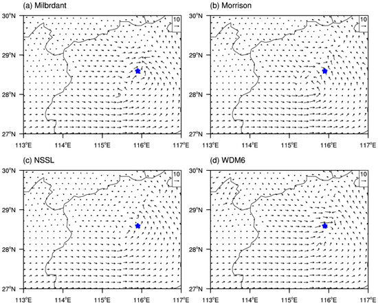
Figure 12.
The 700 hPa storm-relative wind fields at 2230 UTC 15 April 2016 simulated by four double−moment MP schemes (vector, units: m·s−1). The filled blue star is the location of the Nanchang radar station. The square box in the upper-right corner shows 10 m·s−1 wind.
In order to directly reveal the influence of different double-moment MP schemes on wind fields, Figure 13 gives the observed and simulated radar radial velocity at the elevation of 0.5° of the Nanchang radar. The observed radial velocity has a large negative velocity region to the north-west, and the largest radar radial velocity is up to −24 m·s−1, indicating a rear inflow jet. With the WDM6 scheme, there is also one large negative velocity region to the west and south-west, slightly different from the observations, but the largest radar radial velocity is also up to −24 m·s−1. With the other three schemes, there is also one large negative velocity region to the west and south-west, but their intensities are weaker compared with the observations, especially regarding the NSSL scheme. Therefore, the WDM6 scheme generates the strongest rear inflow jet among the four schemes, and the strength of simulated rear inflow matches the observation well.
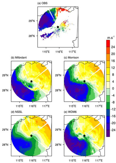
Figure 13.
The radial velocity (shaded, units: m·s−1) at the lowest elevation (0.5°) of the Nanchang radar station with different experiments and the radar observation at 2230 UTC 15 April 2016. The location of the radar station (filled star).
To guarantee the representativeness, Figure 14 shows the vertical cross-section of zonally averaged (10 isometric profiles over 28° N–29° N) wind vectors and perturbation potential temperature at 2230 UTC. A rear inflow jet exists at 800–500 hPa using the Milbrandt, Morrison and WDM6 schemes. For the Milbrandt scheme (Figure 14a), a strong updraft exists in front of the strong convective area from 900 hPa to 300 hPa, which does not seem reasonable, as the observed squall line is about to enter the weakening stage. The simulations with the Morrison scheme (Figure 14b) are similar to those with the Milbrandt scheme, but the strength of the rear inflow jet, updraft and downdraft are all weaker. For the NSSL scheme (Figure 14c), the airflow in the lower layer converges in front of the squall line with weak updrafts and no rear inflow jet, so the simulated squall line does not evolve into a bow-shaped squall line. The rear inflow merges with the cold pool outflow in the WDM6 scheme (Figure 14d), and, furthermore, extends from the middle levels at the back of the squall line to lower levels at the leading region, thus cutting off environment inflow, showing the simulated bow-shaped squall line is in the mature stage and about to enter the weakening stage, which is consistent with the evolution characteristics of the observed squall line.
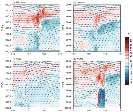
Figure 14.
The vertical cross-section of zonally averaged (10 isometric profiles over 28° N–29° N) wind vectors [vector, (u, 10 w), units: m·s−1] and perturbation potential temperature (shaded, unit: K) at 2230 UTC 15 April 2016 with four different double-moment MP schemes. The red thick line in Figure 14d is the cold pool boundary. The square box in the upper−right corner in (b) shows 10 m·s−1 wind.
4.3. Thermal Characteristics
The cold pool plays an important role in the formation of a bow-shaped squall line [49]. In this paper, the perturbation potential temperature (the potential temperature at each grid point minus the average in the simulated region) at 925 hPa is used to diagnose the cold pool. Figure 15 shows the perturbation potential temperature and wind fields at 925 hPa with the four different double-moment MP schemes at 2230 UTC 15 April 2016. For the Milbrandt scheme (Figure 15a), the strong convective area corresponds to low disturbance potential temperature, and the cold pool is accompanied by cold pool outflows perpendicular to the strong convection line. However, the range of the cold pool is small and its intensity is weak, and the cold pool outflows are also weak. The lowest perturbation potential temperature is only −2 K. There is only a small range of cold pool using the Morrison scheme, but no cold pool outflows perpendicular to the strong convective line (Figure 15b), which may be one reason that the structure of the simulated bow-shaped squall line is very loose. The NSSL scheme (Figure 15c) does not generate an obvious cold pool or cold pool outflows, which can be one reason that the simulated squall line does not evolve into a bow-shaped squall line. The cold pool simulated by the WDM6 scheme (Figure 15d) is relatively obvious. The strong convective area corresponds to low perturbation potential temperature with the lowest value under −4 K, and, moreover, strong cold pool outflows exist, which all contribute to the simulated squall line evolving into a bow-shaped squall line.
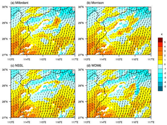
Figure 15.
The 925 hPa wind fields (vector, units: m·s−1) and perturbation potential temperature fields (shaded, unit: K) with four different double−moment MP schemes at 2230 UTC 15 April 2016. The square box in the upper−right corner shows 10 m·s−1 wind.
As shown in Figure 14, the perturbation potential temperatures simulated by the four schemes have a similar spatial structure in the strong convection area with a cold area in the middle and lower layers and a warm area in the middle and upper layers. Among the four schemes, the cold pool simulated by the NSSL scheme is most shallow, and the warm area in the middle and upper layer is the weakest. Compared with the observations, the location of the cold pool is to the west, which obviously lags behind the other three schemes. The strength of the cold pool with the Morrison scheme is weaker than with the Milbrandt scheme, resulting in a weaker simulated bow-shaped squall line. The cold pool simulated by the WDM6 has the largest range and the strongest intensity, with the lowest potential temperature of under −6 K. The reason is that the simulated strong rear inflow directly transports cold air from the middle layers to the lower layers in the convection area, intensifying evaporative rate and cooling effect. Then, the strongest cold pool and cold pool outflow are generated, and eventually the straight squall line evolves into a bow-shaped one.
4.4. Distribution Characteristics of Hydrometeors
To further explore possible reasons why the evolution and structure of the simulated squall lines are different with the four double-moment MP schemes, we present the vertical profiles of domain-averaged hydrometeor mixing ratio simulated by each scheme at 2230 UTC 15 April 2016 in strong convective areas (Figure 16 and Figure 17). We define the strong convective area based on previous study [50,51,52,53,54].
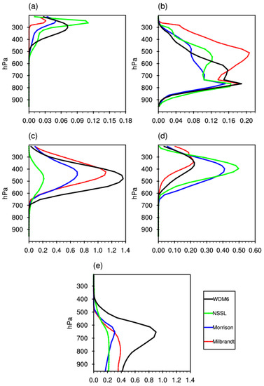
Figure 16.
Vertical profiles of domain−averaged hydrometeors mixing ratio (units: g·kg−1) in strong convective areas with four different double-moment MP schemes at 2230 UTC 15 April 2016. (a) ice, (b) cloud water, (c) graupel, (d) snow, (e) rain water (black line: WDM6 scheme, green line: NSSL scheme, blue line: Morrison scheme, red line: Milbrandt scheme).
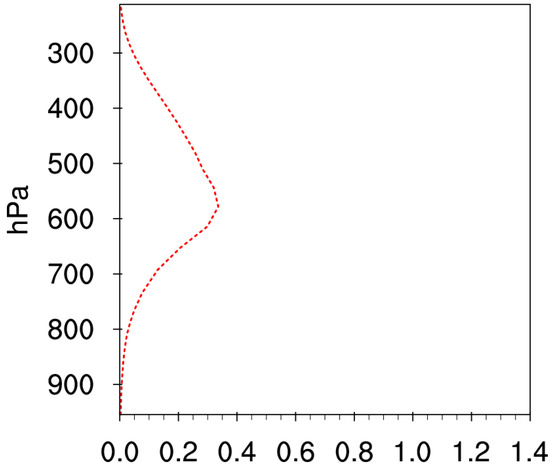
Figure 17.
Vertical profile of domain−averaged hail mixing ratio (units: g·kg−1) in strong convective areas in Milbrandt MP schemes at 2230 UTC 15 April 2016.
In strong convective areas, it can be found that the mixing ratio of snow and graupel in the upper troposphere is much larger than for ice. The mixing ratio of graupel is the largest, except for the NSSL scheme, in which the snow mixing ratio is the largest. Cloud water exists in the upper troposphere, indicating the existence of super cold water in the four schemes. The curves of cloud water mixing ratio almost overlap in the four schemes below 800 hPa. For the WDM6 scheme, the rain water mixing ratio is the largest among the four schemes. The rain water mixing ratio increases rapidly from 400 hPa to 650 hPa and reduces quite rapidly below 650 hPa compared with the other three schemes, representing a large amount of rain water evaporative cooling during the falling process. Therefore, the WDM6 scheme produces the strongest cold pool and rear inflow jet, which is consistent with the simulation results described above. The layers where rain water rapidly increases correspond with those in which both graupel and snow rapidly decrease. Therefore, the rain water mainly comes from the melting of graupel and snow, and the melting of graupel contributes the most.
For the Milbrandt scheme, the distribution of rain water is different from the WDM6 scheme, with a slow decrease under 650 hPa, but a large amount of hail decreases under 650 hPa (Figure 17), so the melting of hail and the evaporation of rain water coexist, which both contribute to the formation of the cold pool and rear inflow jet. The reason may be that graupel and hail are separated from each other and coexist only in the Milbrandt scheme. The density of hail is much larger than graupel and the falling velocity is also much faster than graupel, so that hail can fall below 650 hPa and melt to rain water. Besides, the mixing ratio of snow and graupel in the Milbrandt scheme is smaller than in the WDM6 scheme, but the mixing ratio of the rimed ice particle in both schemes is almost equal and the distribution characteristics of the rimed ice particle in the Milbrandt scheme are similar to the WDM6 scheme. Therefore, rain water in this scheme mainly comes from the melting of graupel, hail and snow. The hail melts to rain below 650 hPa, so the decrease in the rate of rain water under 650 hPa is slow.
For the Morrison scheme, the distribution of rain water is similar to the WDM6 scheme with a decrease under 650 hPa, but the mixing ratio of rain water is lower than for the WDM6 scheme in all layers and the decrease rate is far smaller than for the WDM6 scheme, thus forming a relatively weaker cold pool and rear inflow compared with the WDM6 and Milbrandt. The simulation results of the NSSL scheme are significantly different from the other three schemes. The rainwater mixing ratio is very low and hardly decreases below 650 hPa and no ice phase particles exists below 650 hPa. Therefore, the rainwater evaporation is very small, and no obvious cold pool and rear inflow jet form, which is consistent with the simulation results described above. Furthermore, the content of ice phase particles in the upper troposphere is rather low, and especially the mixing ratio of graupel is obviously lower than for the other schemes.
Double-moment bulk MP schemes can simultaneously predict both the mixing ratio of the hydrometeors and their number concentrations. Vertical profiles of domain-averaged rain water number concentration at 2230 UTC 15 April 2016 with the four different double-moment MP schemes in strong convective areas are shown in Figure 18. It can be seen that the rain water number concentration in the WDM6 scheme is nearly a dozen times larger than for the other three schemes, and the mixing ratio of rain water in the WDM6 scheme is also the largest (Figure 16e). Therefore, the rain water simulated by the WDM6 scheme has minimum volume and the largest surface area, which might help to produce more evaporation of rain water and formation of a stronger cold pool, and successfully simulate the process of the straight squall line evolving into the bow-shaped squall line.
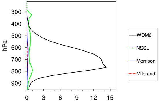
Figure 18.
Vertical profiles of domain-averaged rain water number concentration (units: 104 kg−1) with four different double−moment MP schemes at 2230 UTC 16 April 2016 in strong convective areas. (black line: WDM6, green line: NSSL, blue line: Morrison, red line: Milbrandt).
5. Summary
In this study, the bow-shaped squall line that occurred in East China on 15 April 2016 is simulated using four different double-moment MP schemes (Milbrandt, Morrison, NSSL and WDM6) in WRF. To reduce the impact of initial condition uncertainties on the simulation, radar reflectivity data were assimilated using the cloud analysis method and radar radial velocity data were assimilated by the GSI-3DVar with IVAP observation operators. Based on the simulation results, the evolution and structural characteristics of the thermodynamics and cloud microphysics of the squall line were analyzed, and the effects of the MP schemes on simulating the processes of a straight squall line evolving into a bow-shaped one were revealed. The main conclusions are summarized as follows:
- (1)
- The evolution process simulated by the four double-moment MP schemes are quite different. The WDM6 scheme can reproduce the process of the straight squall line evolving into a bow-shaped squall line well, in concurrence with the observations. The squall lines simulated by the Milbrandt and Morrison schemes also evolved into bow-shaped squall lines, but the simulated results were different from the observations. The NSSL scheme only simulates a broken straight squall line. Threat Scores and Fractions Skill Scores further show that the WDM6 scheme has the best skill in simulating the strong convective area, followed by the Milbrandt, Morrison, and NSSL scheme.
- (2)
- Simulations with WDM6, Milbrandt and Morrison schemes reasonably produce the cold pool and the rear inflow jet when the squall line evolves into a bow-shaped squall line. However, only with the WDM6 scheme does the rear inflow merge with cold pool outflows and extend from the middle levels at the back of the squall line to lower levels at the leading region, which is consistent with the evolution characteristics of the observed squall line. The cold pool and the rear inflow simulated by Milbrandt scheme are weaker than those by the WDM6 scheme, but strong updraft exists in front of the strong convective area from 900 hPa to 300 hPa, which is not reasonable, because the observed squall line is about to enter the weakening stage. The simulated cold pool and rear inflow with the Morrison scheme is weaker than the Milbrandt scheme. For the NSSL scheme, no obvious cold pool and rear inflow jet were generated.
- (3)
- The vertical distribution of hydrometeors in the strong convective area can be used to explain the different simulated results. For the WDM6 scheme, the simulated rain water has the largest mixing ratio and number concentration and the rain water reduces fastest during the falling process, resulting in the strongest cold pool and rear inflow jet, which help the straight squall line evolve into a bow-shaped squall line. For the Milbrandt scheme, both the mixing ratio and number concentration of rain water is less than for the WDM6 scheme, both hail melting and rain evaporation contribute to the formation of a cold pool and rear inflow jet. The simulated rainwater with the Morrison scheme decreases slowly during the falling process with weaker evaporation cooling and a weaker cold pool, and then a weaker rear inflow compared with the Milbrandt and WDM6 schemes. The distribution of simulated hydrometeors with the NSSL scheme is quite different from the other three schemes. The rainwater mixing ratio is very low and hardly decreases below 650 hPa. The evaporation cooling rate with the NSSL scheme is the minimum among the four schemes, and forms the weakest cold pool and rear inflow, which is an important reason that the squall line always appears as a broken straight squall line, instead of evolving into a bow-shaped squall line.
6. Discussions
Among the four MP schemes, our study indicates that the simulation with the WDM6 scheme can best reproduce the evolution process from a straight squall line to a bow-shaped squall line. However, the result is based on only one bow-shaped squall line happening in an environmental condition different from typical bow-shaped squall lines with a low CAPE and an intense vertical wind shear in East China. Future work should repeat these types of studies for more observation cases happening in different environments, perhaps including high-CAPE and low-shear environments or more. In addition, this paper does not address the difference of microphysical processes, such as cloud droplet activation processes, source and sink of different hydrometeors, latent heat release and absorption rates. Moreover, the four MP schemes could not properly capture the stratiform area and thus further study is needed to clarify the physical reasons. In addition to the MP schemes, the boundary layer parameterization (BLP) scheme also has a great influence on MCS simulations [55,56,57,58,59]. Therefore, future study is also needed to investigate the impact of BLP schemes on the simulation of straight squall lines evolving into bow-shaped squall lines.
Author Contributions
Q.C. analyzed the data and wrote the manuscript; S.Z. designed the experiments; G.L. and Y.Z. review and edit the manuscript; All authors have read and agreed to the published version of the manuscript.
Funding
This work is supported by the Meteorological Scientific Research project of Jiangxi Meteorological Bureau (Improvement and application of radar radial wind assimilation observation operator in GSI); National Natural Science Foundation of china (Grant 41765001); Key research and development project of Jiangxi Province (20202BBGL73063).
Institutional Review Board Statement
Not applicable.
Informed Consent Statement
Not applicable.
Data Availability Statement
The radar data and radiosonde data are provided by the Jiangxi Meteorological Bureau. The NCEP data are openly available https://rda.ucar.edu/data/ds083.2/ (accessed on 23 March 2022).
Acknowledgments
We gratefully acknowledge Xudong Liang (State Key Laboratory of Severe Weather, Chinese Academy of Meteorological Sciences) and Feng Chen (Zhejiang Institute of Meteorological Sciences) for their guidance on radar radial wind assimilation.
Conflicts of Interest
The authors declare no conflict of interest.
References
- Parker, M.E.; Johnson, R.H. Organizational modes of midlatitude mesoscale convective systems. Mon. Weather Rev. 2000, 128, 3413–3436. [Google Scholar] [CrossRef]
- Meng, Z.Y.; Zhang, F.Q.; Markowski, P.; Wu, D.C.; Zhao, K.A. Modeling Study on the Development of a Bowing Structure and Associated Rear Inflow within a Squall Line over South China. J. Atmos. Sci. 2012, 69, 1182–1207. [Google Scholar] [CrossRef] [Green Version]
- Przybylinski, R.W. The bow echo:Observation, numerical simulations, and severe weather detection methods. Mon. Weather Rev. 1995, 10, 203–218. [Google Scholar] [CrossRef]
- Snook, N.; Xue, M.; Jung, Y. Analysis of a Tornadic Mesoscale Convective Vortex Based on Ensemble Kalman Filter Assimilation of CASA X-Band and WSR-88D Radar Data. Mon. Weather Rev. 2011, 139, 3446–3467. [Google Scholar] [CrossRef]
- Tong, M.; Xue, M. Ensemble Kalman filter assimilation of Doppler radar data with a compressible nonhydrostatic model: OSS experiments. Mon. Weather Rev. 2005, 133, 1789–1807. [Google Scholar] [CrossRef] [Green Version]
- Hu, M.; Xue, M.; Brewster, K. 3DVAR and cloud analysis with WSR-88D Leval-II data for the prediction of the Fort Worth, Texas, tornadic thunderstorms. Part II: Impact of radial velocity analysis via 3DVAR. Mon. Weather Rev. 2006, 134, 699–721. [Google Scholar] [CrossRef]
- Xiao, Q.N.; Sun, J.Z. Multiple-Radar data assimilation and short-range quantitative precipitation forecasting of a squall line observed during IHOP_2002. Mon. Weather Rev. 2007, 135, 3381–3404. [Google Scholar] [CrossRef]
- Schenkman, A.D.; Xue, M.; Shapiro, A.; Brewster, K.; Gao, J.D. The analysis and prediction of the 8–9 May 2007 Oklahoma tornadic mesoscale convective system by assimilating WSR-88D and CASA radar data using 3DVAR. Mon. Weather Rev. 2011, 139, 224–246. [Google Scholar] [CrossRef] [Green Version]
- Browning, K.A.; Wexler, R. The determination of kinematic properties of a wind field using Doppler radar. J. Appl. Meteor. 1968, 7, 105–113. [Google Scholar] [CrossRef]
- Liang, X. An integrating velocity–azimuth process single Doppler radar wind retrieval method. J. Atmos. Oceanic. Technol. 2007, 24, 658–665. [Google Scholar] [CrossRef]
- Chen, F.; Liang, X.D.; Ma, H. Application of IVAP-based observation operator in radar radial velocity assimilation: The case of typhoon Fitow. Mon. Weather Rev. 2017, 145, 4187–4203. [Google Scholar] [CrossRef]
- Chen, F.; Dong, M.Y.; Ji, C.X.; Liang, X.D. Improving the simulation of the tornado occurring in Funing on 23 June 201 6 by using radar data assimilation. Acta Meteor. Sin. 2019, 77, 405–426. (In Chinese). [Google Scholar] [CrossRef]
- Houghton, J.T.; Ding, Y.; Griggs, D.J.; Noguer, M.; van der Linden, P.J.; Dai, X.; Maskell, K.; Johnson, C.A. Climate Change 2001: The Scientific Basis; Cambridge University Press: Cambridge, UK; New York, NY, USA, 2001. [Google Scholar]
- Min, K.H.; Choo, S.; Lee, D.; Lee, G. Evaluation of WRF cloud microphysics scheme using radar observations. Weather Forecast. 2015, 30, 1571–1589. [Google Scholar] [CrossRef]
- Lin, Y.L.; Farley, R.D.; Orville, H.D. Bulk parameterization of the snow field in a cloud model. J. Clim. Appl. Meteor. 1983, 22, 1065–1092. [Google Scholar] [CrossRef] [Green Version]
- Tao, W.K.; Simpson, J.; McCumber, M. An ice-water saturation adjustment. Mon. Weaather Rev. 1989, 117, 231–235. [Google Scholar] [CrossRef] [Green Version]
- Hong, S.Y.; Dudhia, J.; Chen, S.H. A revised approach to ice microphysical processes for the bulk parameterization of clouds and precipitation. Mon. Weather Rev. 2004, 132, 103–120. [Google Scholar] [CrossRef]
- Lim, K.S.S.; Hong, S.Y. Development of an effective double-moment cloud microphysicals scheme with prognostic cloud condensation nuclei (CCN)for weather and climate models. Mon. Weather Rev. 2010, 138, 1587–1612. [Google Scholar] [CrossRef] [Green Version]
- Chen, S.H.; Sun, W.Y. A one-dimensional time dependent cloud model. J. Meteor. Soc. Jpn. 2002, 80, 99–118. [Google Scholar] [CrossRef] [Green Version]
- Ferrier, B.S.; Tao, W.K.; Simpson, J. A double-moment multiple-phase four-class bulk ice scheme. Part II: Simulations of convective storms in different large-scale environments and comparisons with other bulk parameterizations. J. Atmos. Sci. 1995, 52, 1001–1033. [Google Scholar] [CrossRef] [Green Version]
- Reisner, J.; Rasmussen, R.M.; Bruintjes, R.T. Explicit forecasting of supercooled liquid water in winter storms using the MM5mesoscale model. Quart. J. Roy. Meteor. Soc. 1998, 124, 1071–1107. [Google Scholar] [CrossRef]
- Bryan, G.H.; Morrison, H. Sensitivity of a simulated squall line to horizontal resolution and parameterization of microphysics. Mon. Weather Rev. 2012, 140, 202–225. [Google Scholar] [CrossRef]
- Morrison, H.; Thompson, G.; Tatarskii, V. Impact of cloud microphysics on the development of trailing stratiform precipitation in a simulated squall line: Comparison of one- and two-moment schemes. Mon. Weather Rev. 2009, 137, 991–1007. [Google Scholar] [CrossRef] [Green Version]
- Hong, S.Y.; Lim, K.S.S.; Lee, Y.H.; Ha, J.C.; Kim, H.W. Evaluation of the WRF double-moment 6-class microphysics scheme for precipitating convection scheme for precipitation convection. Adv. Meteor. 2010, 2010, 1–10. [Google Scholar] [CrossRef] [Green Version]
- Huang, D.L.; Gao, S.B.; Min, J.Z. Impact of different cloud microphysical schemes on a squall line simulation. J. Meteor. Sci. 2017, 37, 173–183. (In Chinese). [Google Scholar] [CrossRef]
- Meng, Z.Y.; Yan, D.C.; Zhang, Y.J. General features of squall lines in east China. Mon. Weather Rev. 2013, 141, 1629–1647. [Google Scholar] [CrossRef]
- Johns, R.H.; Hirt, W.D. Derechos:Widespread convectively induced windstorms. Weather Forecast. 1987, 2, 32–49. [Google Scholar] [CrossRef]
- Johns, R.H.; Howard, K.W.; Maddox, R.A. Conditions Associated with Long-Lived Derechos-An Examination of the Large-Scale Environment. In Proceedings of the 16th Conference on Severe Local Storm, Kananaskis Park, AB, Canada, 22–26 October 1990; pp. 408–412, Preprints. [Google Scholar]
- Weisman, M.L. The genesis of severe, long-lived bow echoes. J. Atmos. Sci. 1993, 50, 645–670. [Google Scholar] [CrossRef]
- Hu, M.; Weygandt, S.; Xue, M.; Benjamin, S. Development and Testing of a New Cloud Analysis Package Using Radar, Satellite, and Surface Cloud Observations within GSI for Initializing Rapid Refresh. In Proceedings of the 22nd Conference on Weather Analysis and Forecastion/18th Conference on Numerical Weather Prediction, Park City, UT, USA, 24–29 June 2007. [Google Scholar]
- Hu, M.; Xue, M.; Brewster, K. 3DVAR and cloud analysis with WSR-88D level II data for the prediction of the Fort Worth, Texas, tornadic thunderstorms. Part I: Cloud analysis and its impact. Mon. Weather Rev. 2006, 134, 675–698. [Google Scholar] [CrossRef]
- Weygandt, S.; Benjamin, S.; Devenyi, D.; Brown, J.; Minnis, P. Cloud and Hydrometeor Analysis Using METAR, Radar, and Satellite Data within the RUC/Rapid-Refresh Model. In Proceedings of the 12th conference on Aviation Range and Aerospace Mereorology, Atlanta, GA, USA, 28 January–2 February 2006. [Google Scholar]
- Kessler, E. On the Distribution and Continuity of Water Substance in Atmospheric Circulations. Meteor. Monogr. 1969, 32, 1–84. [Google Scholar] [CrossRef]
- Ferrier, B.S. A double-moment multiple-phase four-class bulk ice scheme. Part I: Descriotion. J. Atmos. Sci. 1994, 52, 1001–1033. [Google Scholar] [CrossRef] [Green Version]
- Thompson, G.; Rasmussen, R.M.; Manning, K. Explicit forcasts of winter precipitation using an improved bulk microphysics scheme. Part I: Description and sensitivity analysis. Mon. Weather Rev. 2004, 132, 519–542. [Google Scholar] [CrossRef] [Green Version]
- Skamarock, W.C.; Coauthors. A Description of the Advanced Research WRF Version 3; Note NCAR/TN-475+STR; NCAR Tech: Boulder, CO, USA, 2008; p. 113. [Google Scholar]
- Mlawer, E.J.; Taubman, S.J.; Brown, P.D.; Iacono, M.J.; Clough, S.A. Radiative transfer for inhomogeneous atmosphere: RRTM, a validated correlated-k model for the longwave. J. Geophys. Res. 1997, 16, 663–682. [Google Scholar] [CrossRef] [Green Version]
- Dudhia, J. Numerical study of convection observed during the Winter Monsoon Experiment using a mesoscale two dimensional model. J. Atmos. Sci. 1989, 46, 3077–3107. [Google Scholar] [CrossRef]
- Noh, Y.; Cheon, W.G.; Hong, S.Y.; Raasch, S. Improvement of the K-profile model for the planetary boundary layer based on large eddy simulation data. Bound. Layer Meteor. 2003, 107, 401–427. [Google Scholar] [CrossRef] [Green Version]
- Ek, M.B.; Mitchell, K.E.; Lin, Y.; Rogers, E.; Grunmann, P.; Koren, V.; Gayno, G.; Tarpley, J.D. Implementation of Noah land surface model advances in the National Centers for Environmental Prediction operational mesoscale Eta model. J. Geophys. Res. 2003, 108, 8851. [Google Scholar] [CrossRef]
- Jiménez, P.A.; Dudhia, J.; González-Rouco, J.F.; Navarro, J.; Montávez, J.P.; García-Bustamante, E. A revised scheme for the WRF surface layer formulation. Mon. Weather Rev. 2012, 140, 898–918. [Google Scholar] [CrossRef] [Green Version]
- Kain, J.S.; Fritsch, J.M. Convective parameterization for mesoscale models: The Kain–Fritsch scheme. In The Representation of Cumulus Convection in Numerical Models; American Meteorological Society: Boston, MA, USA, 1993; p. 246. [Google Scholar]
- Milbrandt, J.A.; Yau, M.K. Multimoment Bulk Microphysics Parametefization. Part I: Analysis of the Role of the Spectral Shape Parameter. J. Atmos. Sci. 2005, 62, 3051–3064. [Google Scholar] [CrossRef] [Green Version]
- Mansell, E.R.; Ziegler, C.L.; Bruning, E.C. Simulated electrification of a small thunderstorm with two-moment bulk microphysics. J. Atmos. Sci. 2010, 67, 171–194. [Google Scholar] [CrossRef]
- Fan, J.W.; Han, B.; Varble, A.; Morrison, H.; North, K.; Kollias, P.; Chen, B.J.; Dong, X.Q.; Giangrande, S.E.; Khain, A.; et al. Cloud-resolving model intercomparison of MC3E squall line case: Part I-Convective updrafts. J. Geophys. Res. Atmos. 2017, 122, 9351–9378. [Google Scholar] [CrossRef]
- Dawn, S.; Satyanarayana, A.N.V. Sensitivity of cloud microphysical schemes of WRF-ARW model in the simulation of trailing stratiform squall line over the Gangetic West Bengal region. J. Atmos. Solar-Terr. Phys. 2020, 209, 105396. [Google Scholar] [CrossRef]
- Halder, M.; Mukhopadhyay, P. Microphysical processes and hydrometeor distributions associated with thunderstorms over India:WRF(cloud-resolving)simulations and validations using TRMM. Nat. Hazards 2016, 83, 1125–1155. [Google Scholar] [CrossRef]
- Cohard, J.M.; Pinty, J.P. A comprehensive two-moment warm microphysical bulk scheme. I: Description and tests. Quart. J. Roy. Meteorol. Soc. 2000, 126, 1815–1842. [Google Scholar] [CrossRef]
- Wheatley, D.M.; Trapp, R.J.; Atkins, N.T. Radar and damage analysis of severe bow echoes observed during BAMEX. Mon. Weather Rev. 2006, 134, 791–805. [Google Scholar] [CrossRef] [Green Version]
- Houze, R.A., Jr. Observed structure of mesoscale convective systems and implications for large-scale heating. Quart. J. Roy. Meteorol. Soc. 1989, 115, 425–461. [Google Scholar] [CrossRef]
- Houze, R.A., Jr. Structure and dynamics of a tropical squall-line system. Mon. Weather Rev. 1977, 105, 1540–1567. [Google Scholar] [CrossRef] [Green Version]
- Zipser, E. Mesoscale and convective-scale downdrafts as distinct components of squall-line structure. Mon. Weather Rev. 1977, 105, 1568–1589. [Google Scholar] [CrossRef] [Green Version]
- Luo, Y.L.; Wang, Y.; Wang, H.; Zheng, Y.J.; Morrison, H. Modeling convective-stratiform precipitation processes on a Mei-Yu front with the Weather Research and Forecasting model: Comparison with observations and sensitivity to cloud microphysics parameterizations. J. Geophys. Res. 2010, 115, D18117. [Google Scholar] [CrossRef] [Green Version]
- Dong, H.; Xu, H.M.; Luo, Y.L. Effects of cloud condensation nuclei concentration on precipitation in convective permitting simulations of a squall line using WRF model: Sensitivity to cloud microphysical schemes. Chin. J. Atmos. Sci. 2012, 36, 145–169. (In Chinese). [Google Scholar] [CrossRef]
- Xu, L.R.; Zhao, M. The influences of boundary layer parameterization schemes on mesoscale heavy rain system. Adv. Atmos. Sci. 2000, 17, 458–472. [Google Scholar] [CrossRef]
- Wisse, J.S.P.; Arellano, V.G.D. Analysis of the role of the planetary boundary layer schemes during a severe convective storm. Ann. Geophys. 2004, 22, 1861–1874. [Google Scholar] [CrossRef] [Green Version]
- Isidora, J.; William, A.G.; Moti, S.; Brent, S.; Steven, E.K. The impact of different WRF Model physical parameterizations and their interactions on warm season MCS rainfall. Weather Forecast. 2005, 20, 1048–1060. [Google Scholar] [CrossRef]
- Wu, D.C.; Meng, Z.Y.; Yan, D.C. The predictability of a squall line in south China on 23 April 2007. Adv. Atmos. Sci. 2013, 30, 485–502. [Google Scholar] [CrossRef]
- Madhulatha, A.; Rajeevan, M. Impact of different parameterization schemes on simulation of mesoscale convective system over south-east India. Meteor. Atmos. Phys. 2018, 130, 49–65. [Google Scholar] [CrossRef]
Publisher’s Note: MDPI stays neutral with regard to jurisdictional claims in published maps and institutional affiliations. |
© 2022 by the authors. Licensee MDPI, Basel, Switzerland. This article is an open access article distributed under the terms and conditions of the Creative Commons Attribution (CC BY) license (https://creativecommons.org/licenses/by/4.0/).