Abstract
Three Microwave Radiation Imagers (MWRI) were carried onboard the FengYun-3B/C/D satellites and have collected more than 10 years of data since 2010. To create a robust climate quality of data, MWRI level one data were reprocessed with new calibration. This study evaluates the performance of retrieving global soil moisture from recalibrated MWRI data (RCD) and quantifies the difference of retrieved soil moisture between operational calibration data (OCD) and RCD. Soil Moisture Operational Products System (SMOPS) products from NOAA on four days of different seasons were collocated with MWRI brightness temperatures, and then the collocated data were used for training an algorithm through machine learning. The retrieved soil moisture products using OCD and RCD were evaluated against the independent SMOPS products, in situ networks and SMAP soil moisture product. It is shown that the algorithm from the random forest is suitable for FY-3D recalibrated MWRI data, with a coefficient of determination (R2) of 0.7223, a mean bias of −0.0062 and an unbiased root mean square difference (ubRMSD) of 0.0476 m3 m−3 compared with SMOPS products over the period from 12 July 2018 to 31 December 2019. The difference of retrieved soil moisture using OCD and RCD is spatially heterogeneous. Both temporal and spatial coverage and accuracy of the existing FY-3D operational soil moisture products are significantly improved.
1. Introduction
Soil moisture (SM) plays an important role in the global water and energy cycle between the atmosphere and Earth’s surface [1]. Knowledge of the spatiotemporal distribution of land SM can help us better understand surface runoff, terrestrial evapotranspiration, rainfall infiltration, soil biochemical and nutrient cycling processes [2,3]. Furthermore, accurate monitoring of SM at various spatiotemporal scales can benefit a variety of applications, such as drought monitoring [4,5,6], rice mapping [7,8], flood warning and forecasting [9,10,11] and irrigation management [12,13]. Despite its extensive applications, obtaining SM with high temporal and spatial coverage and high precision is challenging.
With the rapid development of remote sensing technology, SM can be retrieved by a variety of algorithms from the measurements made at visible to near infrared, thermal infrared to microwave wavelengths [14,15,16,17]. However, microwave remote sensing, especially from passive technology, is still the most effective method for obtaining SM information at regional or global scales due to the relationship between the observed brightness temperature (TB).(TB) and soil dielectric constant [18,19,20]. According to the band setting, the currently available satellite microwave radiometers are generally divided into two categories. One contains a single L-band (1–2 GHz), such as Soil Moisture and Ocean Salinity (SMOS) and Soil Moisture Active Passive (SMAP). The other contains multiple microwave bands (C-, X-, Ku-, K-, Ka- and W-band) in dual polarization states, such as Advanced Microwave Scanning Radiometer–Earth Observing System (AMSR-E), Advanced Microwave Scanning Radiometer2 (AMSR2) and Wind Satellite (WindSat). Because of its better penetration of vegetation and higher sensitivity to SM, the L-band is considered the best band for retrieving SM [21]. In contrast, the high-frequency channels have low sensitivity to SM even under a small fraction of vegetation coverage, leading to high SM retrieval errors. At present, many algorithms have been proposed for L-band SM retrieval, including the L-band microwave emission of biosphere model [22,23], the single channel algorithm at horizontal or vertical polarization [24,25], the dual channel algorithm [26,27], and the land parameter retrieval model [28]. Based on these algorithms, several global SM products and datasets have been published, such as SMOS, SMAP, AMSR-E, AMSR2 Advanced Scatterometer (ASCAT) and the European Space Agency Climate Change Initiative (ESA CCI). These data have brought great benefits to agricultural and hydrological monitoring, weather forecasting, and climate change research [29,30,31]. However, SM retrieval based on a radiative transfer model using L-band requires a lot of auxiliary information, such as the vegetation optical thickness, vegetation single scattering albedo, soil effective temperature, and soil surface roughness, which limits the global application of these methods [32].
Although the inversion method based on physical models has been developed to estimate SM from the multi-channel radiometers with C-band and/or X-band, greater uncertainties can arise due to their low sensitivity to SM and effects of vegetation and surface roughness [33]. The Chinese FengYun-3D (FY-3D) satellite, launched in November 2017, is equipped with a dual-polarization and multifrequency microwave radiometer (MWRI) with frequencies ranging from 10.65 (X-band) to 89 (W-band) GHz. Because FY-3D MWRI lacks the L- and C-bands, more interference factors need to be considered in retrieving SM when the tau–omega radiative transfer model is used for inversion [34,35]. The lowest frequency at X-band available from FY3-D MWRI provides the most SM information; other higher frequencies contain more vegetation signal. Thus, a statistical model is being developed for SM from MWRI.
Machine-learning techniques were used for SM retrieval at different scales based on passive microwave observations [36,37,38,39,40,41,42,43,44]. The method first establishes relationships between the input data (TB and/or ancillary data) and target SM using a variety of algorithms. The reference SM comes from physical model simulations, ground measurements, satellite products, and European Centre for Medium-Range Weather Forecasts model predictions. Al-Yaari et al. [36] constructed a physically-based regression equation using SMOS level three SM and horizontal and vertical TB observations to derive global SM with SMAP level three TBs with the correlation coefficient (R) between 0.51 and 0.84. Santi et al. [37] estimated SM with both satellite-observed and simulated C-band TB based on an artificial neural network algorithm with the statistical parameters of determination of coefficient (R2) of 0.82, root mean square error (RMSD) of 0.035 m−3 m−3 and bias of 0.09 m−3 m−3. However, most of these studies are only based on a single band or two bands such as L- and C-bands or a combination of C-band and X-band. The potential of using the observed TBs in all channels of spaceborne microwave radiometer to estimate SM has not been fully explored.
To deeply mine the historical data resources of multiple series of domestic satellites such as meteorology, land and ocean and build a long-term climate observation plan from the FengYun satellite series, the level 0 observation data of various sensors have been recalibrated with the support of the National Key Research and Development Plan program. The MWRI has been launched on board FY-3 B/C/D satellites, and it is now very conducive to the establishment of a long-term SM dataset. Due to the uncertainty in characterizing receiver nonlinearity, antenna gains and emission during its in-orbit operation, the current FY-3D MWRI operational calibration data (OCD) need to be recalibrated to ensure the stability of long-term data. Recalibrated data (RCD) have been improved mainly in four aspects: thermal mirror emissivity, antenna back lobe, heat source efficiency and receiver nonlinearity [45]. Therefore, it is necessary to evaluate the accuracy difference of SM retrieval based on these two data sources before constructing a long-term global SM dataset.
The objective of this study is to retrieve global SM with the FY-3D recalibrated MWRI data based on a machine-learning algorithm and to evaluate the accuracy difference of SM inversion using FY-3D MWRI OCD and RCD. The paper is structured as follows: In Section 2, the details of our method and the preprocessing of data are introduced. The retrieved soil moistures are analyzed and validated in Section 3. The final conclusion is given in Section 4.
2. Materials and Methods
2.1. FY-3D MWRI Data
FY-3D MWRI measures TBs at five frequencies of 10.65 (X-band), 18.7 (Ku band), 23.8 (K band), 36.5 (Ka band) and 89.0 (W band) GHz with both vertical and horizontal polarization. The antenna scans conically at a fixed viewing angle of 53.4 degrees across a 1400 km swath. The spatial resolution at the surface varies from approximately 70 km at 10.65 Ghz to 10 km at 89 GHz. FY-3D operates in a sun-synchronous polar orbit with the ascending node at 14:00 p.m. and descending node at 2:00 a.m. local solar time. Since the FY-3D MWRI level two SM product (FY-3D L2) was available starting from 12 July 2018, the MWRI level one OCD and RCD provided by the National Satellite Meteorological Center at CMA from 12 July 2018, to 31 December 2019, were used for SM retrieval. The fields of level one data used in this study include TBs of 10 channels, latitude, longitude, land cover type obtained from the International Geosphere–Biosphere Programme classification scheme, surface elevation (digital elevation model, DEM) and quality control information.
Other auxiliary variables include microwave polarization difference index (MPDI) and soil porosity. The MPDI is defined as the ratio of the difference between vertically and horizontally polarized TBs to their sum [46,47]. As an indicator of vegetation, MPDI was selected because it is more sensitive to the total water content of the vegetation per unit area and independent of the surface temperature [48]. Soil porosity, as one of the most important physical attributes, refers to the fraction of the total soil volume that is taken up by the pore space [49], and its size determines how well liquids, gases and heat can be stored and transmitted within the soil matrix. A greater porosity often indicates greater storage and transmission ability. Soil porosity obtained from ESA CCI ancillary data which are derived by applying soil water characteristic equations of Saxton and Rawls (2006) [50] to texture data of the Harmonized World Soil Database v1. was used in this study.
Data cleaning needs to be performed for MWRI level one data before entering the random forest model. First, the fractional coverage of land within MWRI field of view (FOV) were defined by land–sea mask data. The observed TBs affected by radio frequency interference (RFI) were then removed by using the spectral difference method [51]. The FOVs with abnormal TB and surface types of forest, closed shrublands, water body, urban and built up, snow and ice and permanent wetlands were also removed. Finally, the properties from the MWRI level one were resampled to 0.25-degree grids for matching the dependent variable using the nearest neighbor search algorithm. To evaluate the performance of the random forest algorithm for SM estimation, the FY-3D MWRI level two operational SM product was used for comparison.
2.2. NOAA Multi-Sensor Soil Moisture Products
NOAA Soil Moisture Operational Products System (SMOPS) products were used as the training target dataset in the machine-learning model due to its high accuracy and temporal resolution as well as high spatial coverage [52]. SMOPS provides a seamless SM map over global land from six satellites, including Global Precipitation Measurement (GPM), SMAP, Global Change Observation Mission 1st-Water (GCOM-W1), SMOS, Meteorological Operational A (Metop-A), and Metop-B. The global SM maps were generated in daily intervals with the most recent 24 h of SM from multiple retrieval algorithms and mapped with a cylindrical projection on a 0.25 × 0.25 degree grid. For each grid point of the map, the output includes SM values as a percentage (vol/vol) of the surface (top 1–5 cm) soil layer with associated quality information and metadata. The daily product is available in netCDF file format.
2.3. Validation Data
Three kinds of SM data were used for verification, including the independent SMOPS SM products, SM observed by China soil moisture automatic station and SMAP SM product. SM from both automatic stations and SMAP were resampled to 0.25-degree grids using the same method as above before validation. The daily mean in situ SM observations at 10-cm depth from 1924 stations were used to validate the estimated SM over the same time period of MWRI level one. SM values outside the range of 0–0.5 m−3·m−3 were removed. To enhance the representativeness of station observation SM as much as possible, gridding was only carried out for the grids with the number of SM observation values greater than three. The SMAP SM product used for validation was SMAP Enhanced L3 Radiometer Global Daily 9 km EASE-Grid Soil Moisture V004. The time period of all validation data covers from 21 July 2018 to 31 December 2019.
2.4. Random Forest Model Construction
The random forest (RF) algorithm was used to model the relationship between TBs, auxiliary variables and target SM due to its popularity and flexibility [53]. When establishing each tree, the RF algorithm randomly and bootstrapping-samples the rows and columns of the training datasets, which makes it not as easy to overfit as the decision tree algorithm. We used the “RandomForest” package developed with R language to construct the RF model. In RF regression, three main hyperparameters need to be optimized during training: ntree (the number of trees), node size (the minimal size of the leaf node) and mtry (the number of features sampled). According to our optimization result, the values of these three parameters were set as 500, 1, and 1/3 of the total number of the variables, respectively.
To reduce overfitting, it is very important to select a representative training dataset to estimate SM. According to the analysis of [54], more random days cannot significantly improve the estimation accuracy of SM. Therefore, MWRI observations, SMOPS and auxiliary data from four random days (31 January, 30 April, 31 July, and 31 October 2018) were used as training datasets to represent seasonal changes in SM as much as possible in this study. The detailed flowchart for the RF model construction and validation is shown in Figure 1.
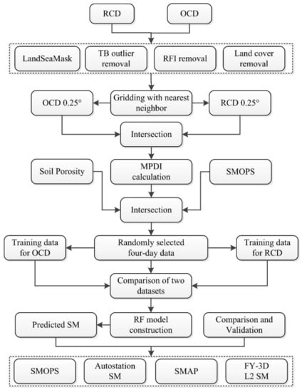
Figure 1.
Flowchart for the RF model construction and validation.
2.5. Evaluation Indicators
To quantitatively evaluate the SM estimated based on OCD and RCD, several statistical metrics were adopted, including the correlation coefficient (R), mean difference (Bias), coefficient of determination (R2) and unbiased root mean square difference (ubRMSD). The formulas for these indicators are as follows:
where n is the number of samples and and are the ith reference and estimated SM, respectively. and are the average of the reference and estimated SM, respectively.
3. Results and Discussion
3.1. Characteristics of Training Dataset from OCD and RCD
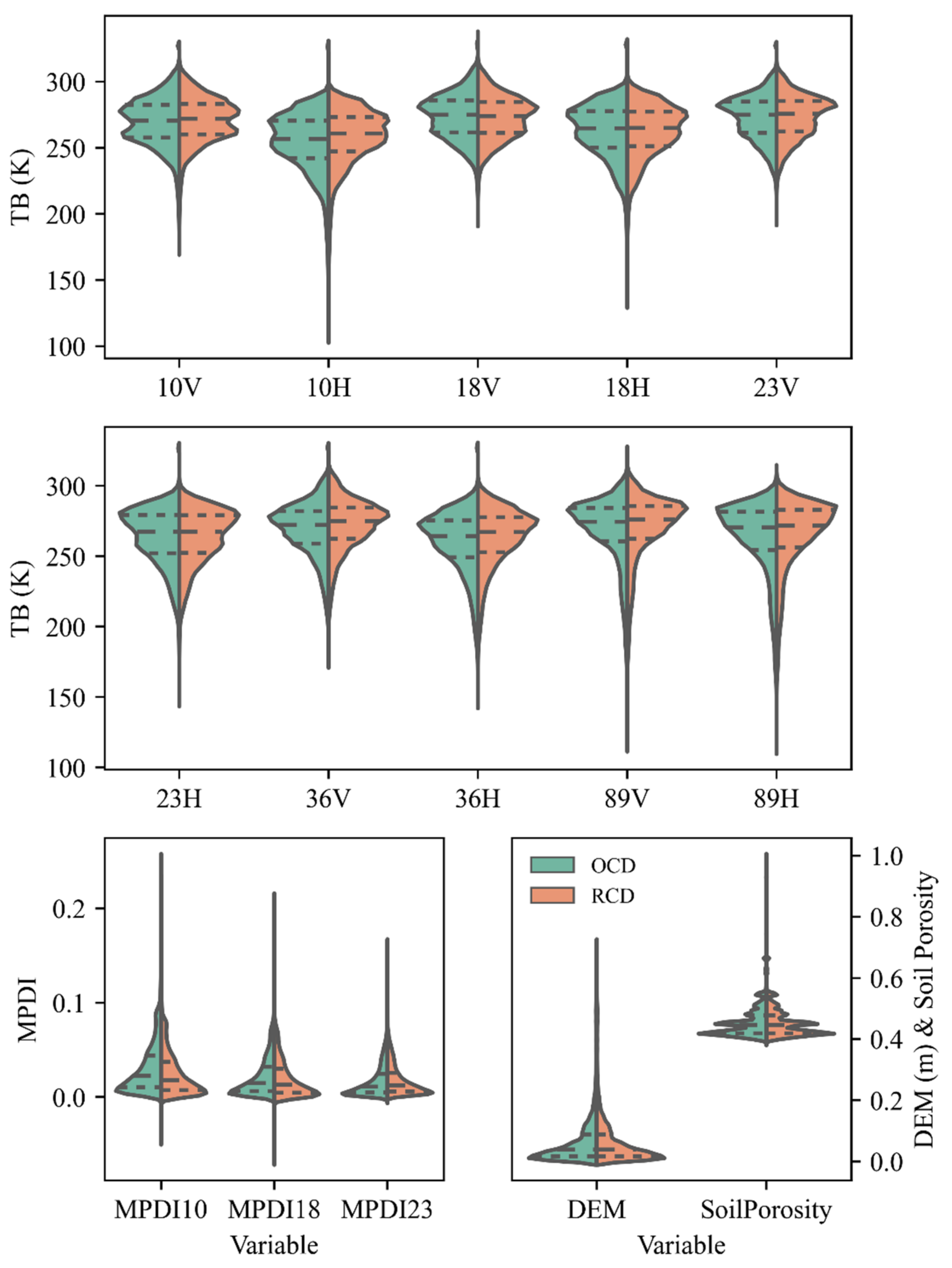
The training dataset was obtained through collocating daily SMOPS and MWRI level one data and soil porosity. Due to the scan pattern offset, the total number of training samples was different between OCD and RCD. Therefore, we resampled the data in space to match the sample size of the two datasets. Finally, 601,974 samples were obtained as a training dataset. The distribution of independent variables in the training datasets is shown in Figure 1. The difference in TBs changes with frequencies. The TBs of all the channels have abnormal values, especially in the low value area. MPDI at all frequencies have the characteristics of unimodal distribution. MPDI at 10 and 18 GHz from OCD are larger than that from RCD, while the difference in MPDI at 23 GHz is small. Abnormal values from MPDI also occur, especially in the high value area. To draw with soil porosity in the same axes, the value of DEM divided by 10,000 is displayed. Due to the preprocess of gridding, the distribution of DEM between OCD and RCD has negligible differences. The statistical distribution of soil porosity between OCD and RCD is almost the same (Figure 2).
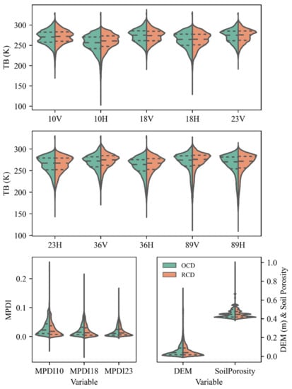
Figure 2.
Distribution of TBs of all channels, MPDI, DEM and soil porosity in training datasets from OCD and RCD. Digit in x label denotes frequency, H and V denote horizontal and vertical polarization, respectively.
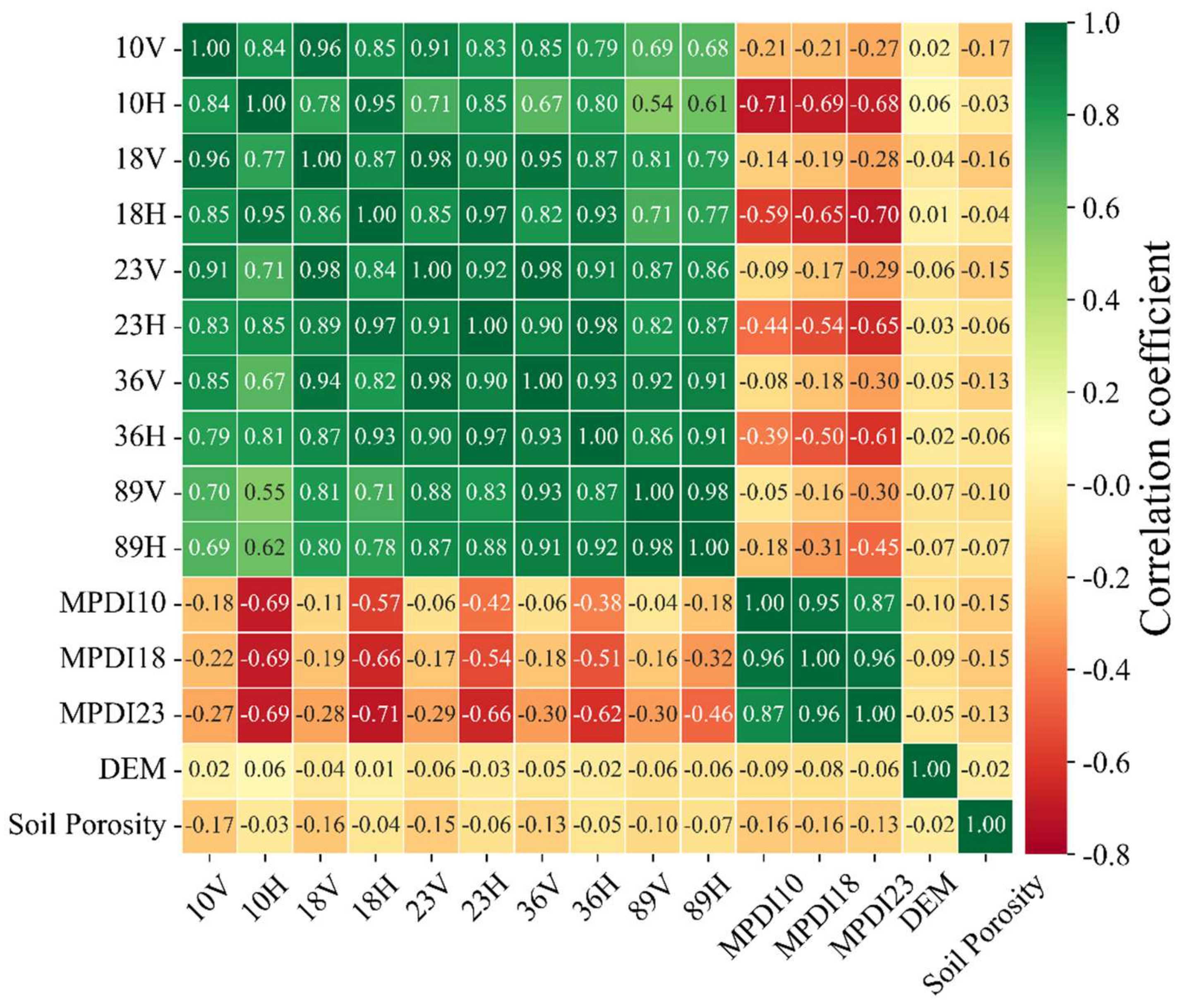
The correlation coefficients between independent variables in OCD and RCD are shown in Figure 3. TBs between different frequencies have a high positive correlation coefficient with the highest R of 0.98 between 23V and 36V and the lowest R of 0.55 between 10H and 89V for RCD. The correlation coefficient decreases with the increase of frequency interval. The correlation coefficients between vertical polarization TBs are greater than that between horizontal polarization TBs. TBs of different frequencies with horizontal polarization have a stronger negative correlation with MPDI than that with vertical polarization. MPDI between different frequencies have high correlation coefficients. Both DEM and soil porosity have low correlation coefficients with other variables. The relationships of independent variables in OCD are similar with that in RCD (Figure 3).

Figure 3.
Correlation coefficient between variables in the training datasets from OCD (upper left triangle) and RCD (lower right triangle).
To further analyze the differences of independent variables in the OCD and RCD training datasets, the average bias was calculated by the variable values of the training datasets of RCD minus that of OCD, and the results are shown in Figure 4. Except for TBs at 18V and 23H, the TBs at other channels have a positive bias, and the maximum positive bias occurs in the channel of 10H with a mean bias of 4.0221 k. The mean biases of MPDI at 10 GHz and 18 GHz are negative, while the mean bias of MPDI at 23 GHz is positive.
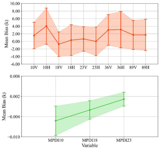
Figure 4.
Mean difference of variables in the training dataset.
3.2. Soil Moisture Retrieved from OCD and RCD
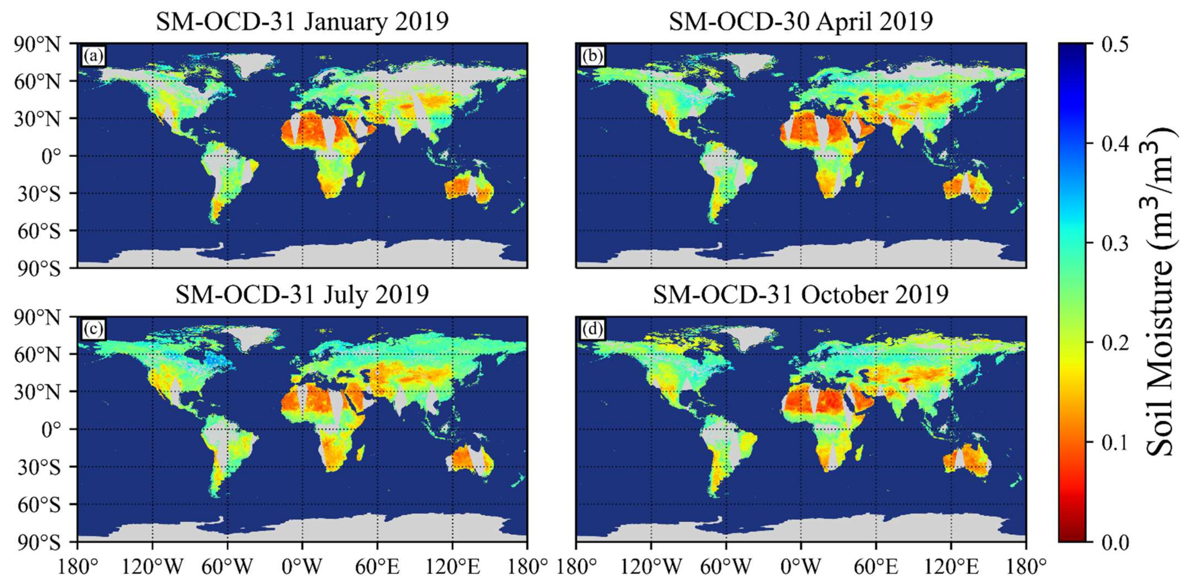
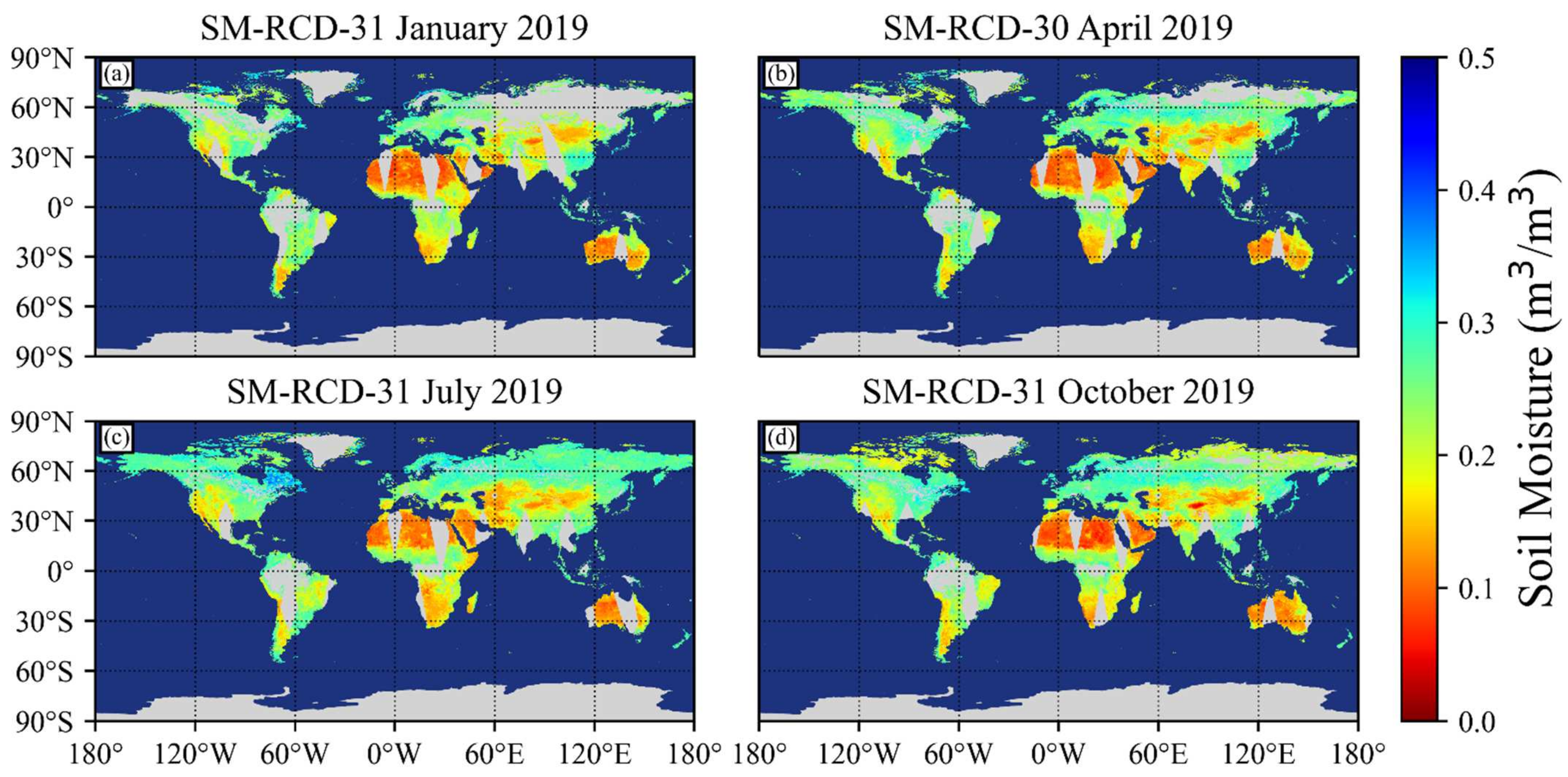
Because of the advantages of fast computation and unbiased estimation, the out of bag error is commonly used to test performance of a RF model [55,56]. The out of bag error of the RF model trained by 500 trees was 0.0398 m3·m−3. To reflect the seasonal variations in SM, the global distribution map of retrieved SM of the four days in 2019 are displayed based on OCD and RCD (Figure 5 and Figure 6). Compared with the existing operational SM product (FY3D L2), the SM obtained by the random forest algorithm has higher spatial and temporal coverage and therefore can enhance the application of SM in the fields of atmosphere, hydrology and environment. However, there are some missing retrievals for SM maps over the northern hemisphere, such as Russia and Canada, particularly in January. There are also some missing retrievals in the tropical region, particularly in the Amazon Forest and Southeast Asia, in all months. This is because the SM on these types of land cover is naturally difficult to retrieve based on microwave remote sensing technology including snow, ice, forest and wetland [57,58].
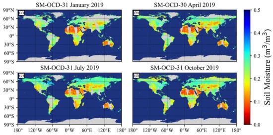
Figure 5.
Global soil moisture maps retrieved based on OCD on: (a) 31 January; (b) 30 April; (c) 31 July; and (d) 31 October 2019.
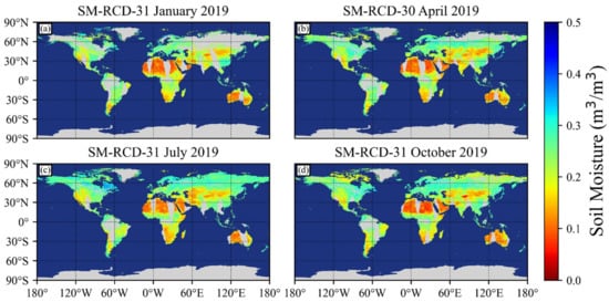
Figure 6.
Global soil moisture maps retrieved based on RCD on: (a) 31 January; (b) 30 April; (c) 31 July; and (d) 31 October 2019.
Over the northern hemisphere, SM increases from winter to summer and begins to decrease in autumn, especially for the North American and Eurasian continents. For the equatorial region, a warm and humid climate brings an increasing trend of SM from the winter to summer seasons. For the southern hemisphere, the seasonal variation in SM is the opposite, particularly for the southern part of the African continent and Australia. On the Australian continent, higher SM can be seen during January, especially over the north coast, when compared with the July map. The southern part of the African continent has similar trends as the Australian continent. SM in desert areas, such as the Sahel, is low throughout the year.
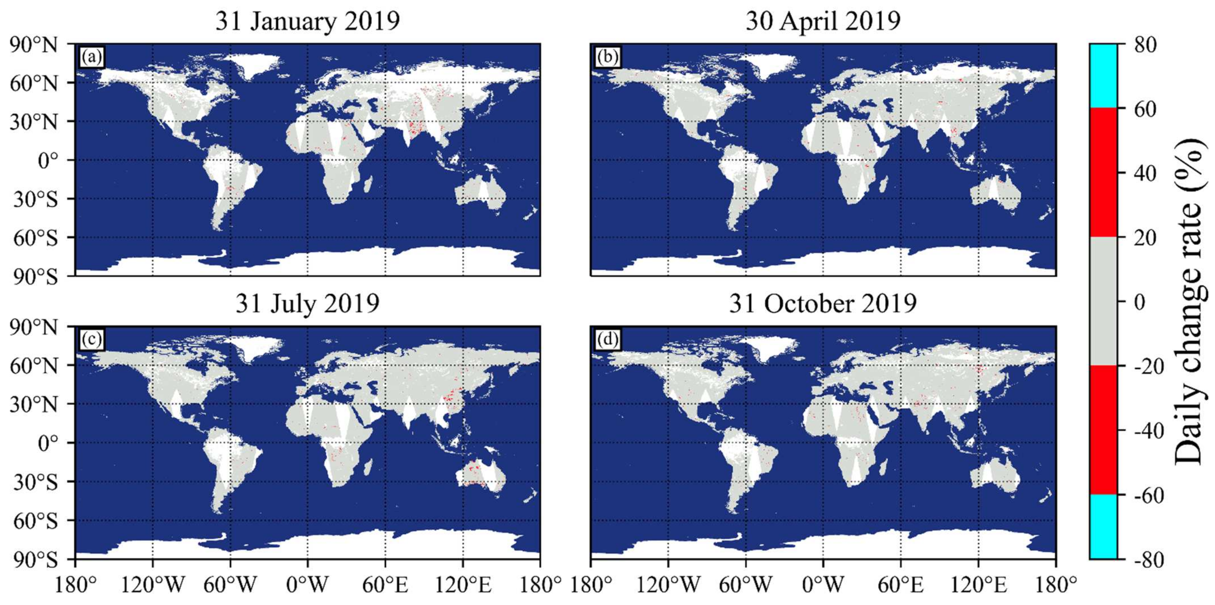
From the SM inversion results (Figure 5 and Figure 6), it can be seen that the temporal and spatial distribution between SM retrieved by OCD and RCD is very similar. To quantitatively show the difference between SM retrieved by OCD and RCD, the SM daily change rate was calculated by subtracting the SM retrieved using OCD from the SM retrieved using RCD and then dividing it by the SM retrieved using OCD. The daily change rate of SM in most areas on the four days was between −20% and 20%; in a few areas, it was between −20% and −60% and 20 to 60% (Figure 7). In particular, on 31 January and 31 July, the variation rate of SM in a few grids was between 60% and 80%. Therefore, the relative change rate of SM is different in time and space. For most regions, the change rate is within 20%.
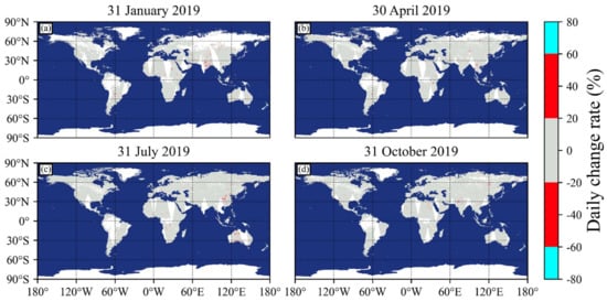
Figure 7.
Soil moisture daily change rate on (a) 31 January, (b) 30 April, (c) 31 July and (d) 31 October of 2019.
3.3. Inversion Accuracy Evaluation
3.3.1. Verification Based on SMOPS Data
The statistical indicators computed using SMOPS products are shown in Figure 8. The accuracy of SM retrieved based on RCD is better than that of the FY3D level two SM product with a mean bias mostly within 0.02, R2 greater than 0.6 and ubRMSD lower than 0.06. The inversion accuracy of SM between OCD and RCD is similar. The statistical metrics are listed in Table 1. Both OCD and RCD have lower negative mean biases values (−0.0062 m3·m−3) than FY-3D L2 (−0.01 m3·m−3). RCD had a higher average R2 value (0.7223) than OCD (0.7193). Both of them have a higher average R2 values than FY-3D L2 (0.4097). In contrast, OCD and RCD have basically the same average ubRMSD values (0.0477, 0.0476), while FY-3D L2 has a higher average ubRMSD value (0.099 m3·m−3).
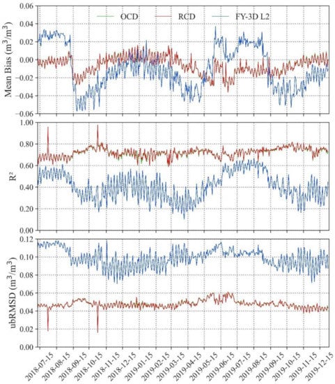
Figure 8.
Validation of soil moisture retrieved using OCD (green line), RCD (red line) and FY-3D L2 (blue line) based on SMOPS products.

Table 1.
Summary of the average validation indicators of soil moisture retrieval SMOPS products.
3.3.2. Verification Based on Automatic Station Data
The statistical indicators computed using in situ SM are shown in Figure 9. The number of matched soil observations in each grid point greater than 30 was used to calculate the statistical metrics. The metrics of the grid with a p value of the correlation coefficient less than 0.01 are displayed. As we can see from the distribution of the R, most of the grids show a positive correlation, and a few grids show a negative correlation. The values and spatial distribution of statistical indicators are basically similar using OCD and RCD. The statistical results of the metrics are listed in Table 2. OCD results in a slightly higher average R value (0.3025) than RCD (0.2952). In contrast, the average of mean bias and ubRMSD from OCD (0.0334, 0.0505) is slightly lower than those from RCD (0.0340, 0.0507). The verification of satellite-based SM using in situ SM is a necessary condition for ensuring the quality of information before being used for various studies. However, due to the differences in penetration depth between ground-based and satellite observations and their spatial representation, it is difficult to obtain more realistic validation results [59,60]. To minimize the representativeness errors, all the stations falling within a particular satellite field of view were (after quality control) averaged by calculating the arithmetic mean [61]. Finally, the mean values of SM observed at three to five automatic stations were used to validate SM retrieved by OCD and RCD.
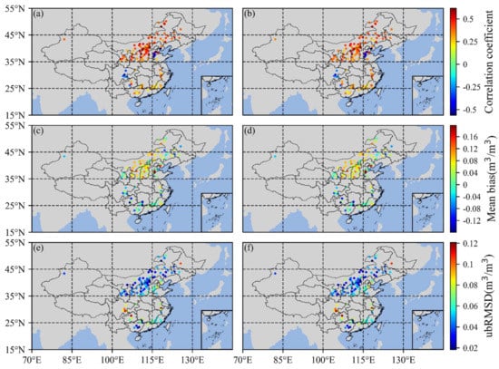
Figure 9.
Validation of soil moisture retrieved using OCD (a,c,e) and RCD (b,d,f) based on autostation observations.

Table 2.
Summary of the average validation indicators of soil moisture retrieval based on in situ soil moisture.
3.3.3. Verification Based on SMAP Soil Moisture Products
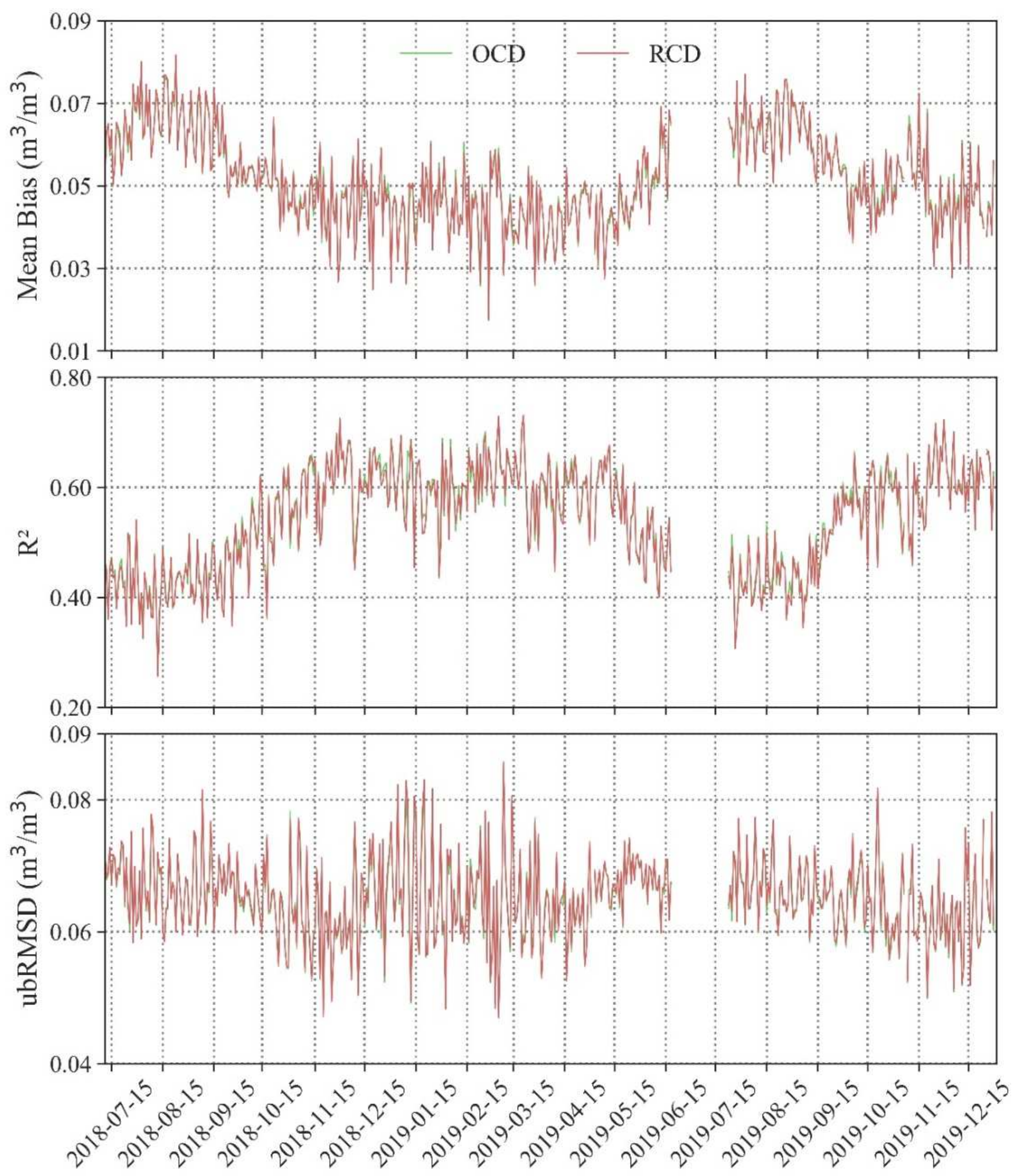
The statistical indicators computed using SMAP SM products are shown in Figure 10. Overall, the change trends of the statistical indicators of SM retrieved using OCD and RCD are basically the same. Due to the lack of SMAP SM products from 20 June to 23 July of 2019, each statistical index is discontinuous. The statistical results of the metrics are listed in Table 3. There is little difference in the statistical results of indicators. SM retrieved based on the random forest algorithm has an average R2 of 0.5421, average mean bias of 0.0514 and average ubRMSD of 0.0653.
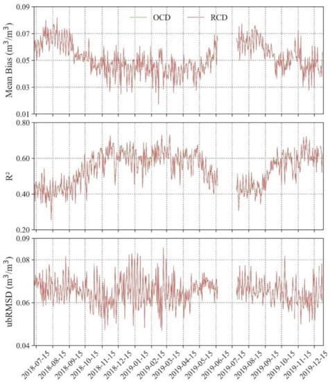
Figure 10.
Validation of soil moisture retrieved using OCD (green line) and RCD (red line) based on SMAP product.

Table 3.
Summary of the average validation indicators of soil moisture retrieval based on SMAP soil moisture products.
The machine-learning technique allows the retrieval of SM from both active and passive satellite systems with an accuracy of approximately 0.05 m3·m−3 of SM or better [37,62,63,64,65]. Our result is in agreement with previous studies. In addition to using polarized TB in different channels, these studies also use auxiliary data, such as the normalized difference vegetation index (NDVI) and land surface temperature (LST). The difference between this study and previous studies is that except for soil porosity, most of the auxiliary data such as DEM and land cover type are included in the FY-3D MWRI level one data. Thus, the implementation of the random forest algorithm using FY-3D MWRI data is more convenient.
4. Conclusions
The performance of global SM retrieval using recalibrated FY-3D MWRI data was evaluated using a multivariable random forest method. The SM retrieved with RCD has a high consistency and accuracy with SMOPS products (R2 = 0.7223, mean bias = −0.0062 and ubRMSD = 0.0476 m3 m−3), the in situ data (R = 0.2952, mean bias = 0.034 and ubRMSD = 0.0507 m3 m−3) and SMAP products (R2 = 0.5421, mean bias = 0.0514 and ubRMSD = 0.0653 m3 m−3). The seasonal distribution of SM at the global scale is reasonable. The accuracy difference of SM retrieved using OCD and RCD was also evaluated using SMOPS products, in situ networks from automatic soil moisture observation stations in China and SMAP SM products. The recalibration of TB data from the FY-3D MWRI had an impact on global SM retrieval with the characteristics of spatial heterogeneity; however, the change rate on most areas is within 20%. The multivariable retrieval method could be applied to all the MWRIs onboard FY-3 satellites since 2010 due to their similar characteristics, which could support the development of a long-term SM product. The newly launched FY-3E satellite carries a microwave scatterometer (WindRad) with a 17:30/05:30 ascending/descending orbit that is operated by the Chinese National Satellite Meteorological Center (NSMC). The WindRad measures the backscattering at C-band (5.3 GHz) and Ku-band (13.265 GHz) with HH and VV polarization for both frequencies. The antenna scans conically at a viewing angle of 36–45 degrees for C-band and 37–43 degrees for Ku-band. Random forest can also be used for retrieving SM based on WindRad Observations. This will provide the SM product at dawn and evening. It is helpful to study the diurnal variation in SM when combined with the SM product derived from MWRI data from FY-3B to 3D.
Author Contributions
Conceptualization, C.W. and F.W.; formal analysis, C.W.; funding acquisition, F.W.; methodology, C.W.; project administration, F.W.; validation, C.W.; writing—original draft, C.W.; writing—review and editing, F.W., S.W., D.W. and P.Z.; resources, S.W. and D.W. All authors have read and agreed to the published version of the manuscript.
Funding
This work was supported by the National Key Research and Development Program of China under the funding code of 2021YFB3900400, the Second Tibetan Plateau Scientific Expedition and Research Program (2019QZKK0105) and the Basic Research Fund of CAMS (2019Y008).
Acknowledgments
The operational calibration and recalibration data of the FY-3D MWRI were provided by NSMC. The FY-3D soil moisture products were also provided by NSMC.
Conflicts of Interest
The authors declare no conflict of interest.
References
- Seneviratne, S.I.; Corti, T.; Davin, E.L.; Hirschi, M.; Jaeger, E.B.; Lehner, I.; Orlowsky, B.; Teuling, A.J. Investigating soil moisture-climate interactions in a changing climate: A review. Earth-Sci. Rev. 2010, 99, 125–161. [Google Scholar] [CrossRef]
- Yang, C.Y.; Ma, Y.M.; Yuan, Y. Terrestrial and Atmospheric Controls on Surface Energy Partitioning and Evaporative Fraction Regimes Over the Tibetan Plateau in the Growing Season. J. Geophys. Res. Atmos. 2021, 126, e2021JD035011. [Google Scholar] [CrossRef]
- Nanda, A.; Sen, S. A complex network theory based approach to better understand the infiltration-excess runoff generation thresholds. J. Hydrol. 2021, 603, 127038. [Google Scholar] [CrossRef]
- Soares Saraiva Souza, A.G.; Ribeiro Neto, A.; de Souza, L.L. Soil moisture-based index for agricultural drought assessment: SMADI application in Pernambuco State-Brazil. Remote Sens. Environ. 2021, 252, 112124. [Google Scholar] [CrossRef]
- Xu, L.; Abbaszadeh, P.; Moradkhani, H.; Chen, N.C.; Zhang, X. Continental drought monitoring using satellite soil moisture, data assimilation and an integrated drought index. Remote Sens. Environ. 2020, 250, 112028. [Google Scholar] [CrossRef]
- Mladenova, I.E.; Bolten, J.D.; Crow, W.T.; Sazib, N.; Cosh, M.H.; Tucker, C.J.; Reynolds, C. Evaluating the Operational Application of SMAP for Global Agricultural Drought Monitoring. IEEE J. Sel. Top. Appl. Earth Obs. Remote Sens. 2019, 12, 3387–3397. [Google Scholar] [CrossRef]
- Wang, Y.; Zang, S.Y.; Tian, Y. Mapping paddy rice with the random forest algorithm using MODIS and SMAP time series. Chaos Solitons Fractals 2020, 140, 110116. [Google Scholar] [CrossRef]
- Kucuk, C.; Taskin, G.; Erten, E. Paddy-Rice Phenology Classification Based on Machine-Learning Methods Using Multitemporal Co-Polar X-Band SAR Images. IEEE J. Sel. Top. Appl. Earth Obs. Remote Sens. 2016, 9, 2509–2519. [Google Scholar] [CrossRef]
- El Khalki, E.M.; Tramblay, Y.; Massari, C.; Brocca, L.; Simonneaux, V.; Gascoin, S.; Saidi, M.E.M. Challenges in flood modeling over data-scarce regions: How to exploit globally available soil moisture products to estimate antecedent soil wetness conditions in Morocco. Nat. Hazards Earth Syst. Sci. 2020, 20, 2591–2607. [Google Scholar] [CrossRef]
- Kim, S.; Paik, K.; Johnson, F.M.; Sharma, A. Building a Flood-Warning Framework for Ungauged Locations Using Low Resolution, Open-Access Remotely Sensed Surface Soil Moisture, Precipitation, Soil, and Topographic Information. IEEE J. Sel. Top. Appl. Earth Obs. Remote Sens. 2018, 11, 375–387. [Google Scholar] [CrossRef]
- Brocca, L.; Ciabatta, L.; Massari, C.; Moramarco, T.; Hahn, S.; Hasenauer, S.; Kidd, R.; Dorigo, W.; Wagner, W.; Levizzani, V. Soil as a natural rain gauge: Estimating global rainfall from satellite soil moisture data. J. Geophys. Res.-Atmos. 2014, 119, 5128–5141. [Google Scholar] [CrossRef]
- Jalilvand, E.; Tajrishy, M.; Hashemi, S.A.G.Z.; Brocca, L. Quantification of irrigation water using remote sensing of soil moisture in a semi-arid region. Remote Sens. Environ. 2019, 231, 111226. [Google Scholar] [CrossRef]
- Chen, Y.L.; Lu, D.S.; Luo, L.F.; Pokhrel, Y.; Deb, K.; Huang, J.F.; Ran, Y.H. Detecting irrigation extent, frequency, and timing in a heterogeneous arid agricultural region using MODIS time series, Landsat imagery, and ancillary data. Remote Sens. Environ. 2018, 204, 197–211. [Google Scholar] [CrossRef]
- Peng, J.; Albergel, C.; Balenzano, A.; Brocca, L.; Cartus, O.; Cosh, M.H.; Crow, W.T.; Dabrowska-Zielinska, K.; Dadson, S.; Davidson, M.W.J.; et al. A roadmap for high-resolution satellite soil moisture applications—Confronting product characteristics with user requirements. Remote Sens. Environ. 2021, 252, 112162. [Google Scholar] [CrossRef]
- Li, Z.L.; Leng, P.; Zhou, C.H.; Chen, K.S.; Zhou, F.C.; Shang, G.F. Soil moisture retrieval from remote sensing measurements: Current knowledge and directions for the future. Earth-Sci. Rev. 2021, 218, 103673. [Google Scholar] [CrossRef]
- Babaeian, E.; Sadeghi, M.; Jones, S.B.; Montzka, C.; Vereecken, H.; Tuller, M. Ground, Proximal, and Satellite Remote Sensing of Soil Moisture. Rev. Geophys. 2019, 57, 530–616. [Google Scholar] [CrossRef]
- Petropoulos, G.P.; Ireland, G.; Barrett, B. Surface soil moisture retrievals from remote sensing: Current status, products & future trends. Phys. Chem. Earth 2015, 83–84, 36–56. [Google Scholar] [CrossRef]
- Wigneron, J.P.; Calvet, J.C.; De Rosnay, P.; Kerr, Y.; Waldteufel, P.; Saleh, K.; Escorihuela, M.J.; Kruszewski, A. Soil Moisture Retrievals From Biangular L-Band Passive Microwave Observations. IEEE Geosci. Remote Sens. Lett. 2004, 1, 277–281. [Google Scholar] [CrossRef]
- Schmugge, T. Remote sensing of surface soil moisture. J. Appl. Meteorol. 1978, 17, 1549–1557. [Google Scholar] [CrossRef]
- Njoku, E.G.; Kong, J.A. Theory for passive microwave remote sensing of near-surface soil moisture. J. Geophys. Res. 1977, 82, 3108–3118. [Google Scholar] [CrossRef]
- Calvet, J.C.; Wigneron, J.P.; Walker, J.; Karbou, F.; Chanzy, A.; Albergel, C. Sensitivity of Passive Microwave Observations to Soil Moisture and Vegetation Water Content: L-Band to W-Band. IEEE Trans. Geosci. Remote Sens. 2011, 49, 1190–1199. [Google Scholar] [CrossRef]
- Wigneron, J.P.; Kerr, Y.; Waldteufel, P.; Saleh, K.; Escorihuela, M.J.; Richaume, P.; Ferrazzoli, P.; de Rosnay, P.; Gurney, R.; Calvet, J.C.; et al. L-band Microwave Emission of the Biosphere (L-MEB) Model: Description and calibration against experimental data sets over crop fields. Remote Sens. Environ. 2007, 107, 639–655. [Google Scholar] [CrossRef]
- Kerr, Y.H.; Waldteufel, P.; Richaume, P.; Wigneron, J.-P.; Ferrazzoli, P.; Mahmoodi, A.; Al Bitar, A.; Cabot, F.; Gruhier, C.; Juglea, S.E.; et al. The SMOS Soil Moisture Retrieval Algorithm. IEEE Trans. Geosci. Remote Sens. 2012, 50, 1384–1403. [Google Scholar] [CrossRef]
- Gao, L.; Ebtehaj, A.; Chaubell, M.J.; Sadeghi, M.; Li, X.J.; Wigneron, J.P. Reappraisal of SMAP inversion algorithms for soil moisture and vegetation optical depth. Remote Sens. Environ. 2021, 264, 112627. [Google Scholar] [CrossRef]
- Judge, J.; Liu, P.W.; Monsivais-Huertero, A.; Bongiovanni, T.; Chakrabarti, S.; Steele-Dunne, S.C.; Preston, D.; Allen, S.; Bermejo, J.P.; Rush, P.; et al. Impact of vegetation water content information on soil moisture retrievals in agricultural regions: An analysis based on the SMAPVEX16-MicroWEX dataset. Remote Sens. Environ. 2021, 265, 112623. [Google Scholar] [CrossRef]
- Konings, A.G.; Piles, M.; Das, N.; Entekhabi, D. L-band vegetation optical depth and effective scattering albedo estimation from SMAP. Remote Sens. Environ. 2017, 198, 460–470. [Google Scholar] [CrossRef]
- Chaubell, M.J.; Yueh, S.H.; Dunbar, R.S.; Colliander, A.; Chen, F.; Chan, S.K.; Entekhabi, D.; Bindlish, R.; O’Neill, P.E.; Asanuma, J.; et al. Improved SMAP Dual-Channel Algorithm for the Retrieval of Soil Moisture. IEEE Trans. Geosci. Remote Sens. 2020, 58, 3894–3905. [Google Scholar] [CrossRef]
- Zhao, T.J.; Hu, L.; Shi, J.C.; Lu, H.S.; Li, S.N.; Fan, D.; Wang, P.K.; Geng, D.Y.; Siang, C.K.; Zhang, Z.Q. Soil moisture retrievals using L-band radiometry from variable angular ground-based and airborne observations. Remote Sens. Environ. 2020, 248, 111958. [Google Scholar] [CrossRef]
- Crow, W.T. Hydrologic applications for SMAP and SMOS surface soil moisture retrieval products. In Proceedings of the IGARSS 2017—2017 IEEE International Geoscience and Remote Sensing Symposium, Fort Worth, TX, USA, 23–28 July 2017. [Google Scholar]
- Mishra, A.; Vu, T.; Veettil, A.V.; Entekhabi, D. Drought monitoring with soil moisture active passive (SMAP) measurements. J. Hydrol. 2017, 552, 620–632. [Google Scholar] [CrossRef]
- Chakraborty, A.; Seshasai, M.V.R.; Murthy, C.S.; Kameswara Rao, S.V.C. Assessing early season drought condition using AMSR-E soil moisture product. Geomat. Nat. Hazards Risk 2013, 4, 164–186. [Google Scholar] [CrossRef][Green Version]
- Panciera, R.; Walker, J.P.; Kalma, J.D.; Kim, E.J.; Saleh, K.; Wigneron, J.P. Evaluation of the SMOS L-MEB passive microwave soil moisture retrieval algorithm. Remote Sens. Environ. 2009, 113, 435–444. [Google Scholar] [CrossRef]
- Schmugge, T.; Gloersen, P.; Wilheit, T. Remote Sensing of Soil Moisture with Microwave Radiometers; NASA Technical Note D-8321; NASA: Washington, DC, USA, 1976.
- Kang, C.S.; Zhao, T.J.; Shi, J.C.; Cosh, M.H.; Chen, Y.Y.; Starks, P.J.; Collins, C.H.; Wu, S.L.; Sun, R.J.; Zheng, J.Y. Global Soil Moisture Retrievals From the Chinese FY-3D Microwave Radiation Imager. IEEE Trans. Geosci. Remote Sens. 2020, 59, 4018–4032. [Google Scholar] [CrossRef]
- Mo, T.; Choudhury, B.J.; Schmugge, T.J.; Wang, J.R.; Jackson, T.J. A model for microwave emission from vegetation-covered fields. J. Geophys. Res. Ocean. 1982, 87, 11229–11237. [Google Scholar] [CrossRef]
- Al-Yaari, A.; Wigneron, J.P.; Kerr, Y.; Rodriguez-Fernandez, N.; O’Neill, P.E.; Jackson, T.J.; De Lannoy, G.J.M.; Al Bitar, A.; Mialon, A.; Richaume, P.; et al. Evaluating soil moisture retrievals from ESA’s SMOS and NASA’s SMAP brightness temperature datasets. Remote Sens. Environ. 2017, 193, 257–273. [Google Scholar] [CrossRef]
- Santi, E.; Paloscia, S.; Pettinato, S.; Fontanelli, G. Application of artificial neural networks for the soil moisture retrieval from active and passive microwave spaceborne sensors. Int. J. Appl. Earth Obs. Geoinf. 2016, 48, 61–73. [Google Scholar] [CrossRef]
- Al-Yaari, A.; Wigneron, J.P.; Kerr, Y.; Rodriguez-Fernandez, N.; O’Neill, P.E.; Jackson, T.J.; De Lannoy, G.J.M.; Al Bitar, A.; Mialon, A.; Richaume, P.; et al. First application of regression analysis to retrieve Soil Moisture from SMAP brightness temperature observations consistent with SMOS. In Proceedings of the 2016 IEEE International Geoscience and Remote Sensing Symposium (IGARSS), Beijing, China, 10–15 July 2016; pp. 1633–1636. [Google Scholar]
- Al-Yaari, A.; Wigneron, J.P.; Kerr, Y.; de Jeu, R.; Rodriguez-Fernandez, N.; van der Schalie, R.; Al Bitar, A.; Mialon, A.; Richaume, P.; Dolman, A.; et al. Testing regression equations to derive long-term global soil moisture datasets from passive microwave observations. Remote Sens. Environ. 2016, 180, 453–464. [Google Scholar] [CrossRef]
- Rodriguez-Fernandez, N.J.; Aires, F.; Richaume, P.; Kerr, Y.H.; Prigent, C.; Kolassa, J.; Cabot, F.; Jimenez, C.; Mahmoodi, A.; Drusch, M. Soil Moisture Retrieval Using Neural Networks: Application to SMOS. IEEE Trans. Geosci. Remote Sens. 2015, 53, 5991–6007. [Google Scholar] [CrossRef]
- Angiuli, E.; Frate, F.D.; Monerris, A. Application of Neural Networks to Soil Moisture Retrievals from L-Band Radiometric Data. In Proceedings of the IGARSS 2008—2008 IEEE International Geoscience and Remote Sensing Symposium, Boston, MA, USA, 7–11 July 2008. [Google Scholar]
- Frate, F.D.; Ferrazzoli, P.; Schiavon, G. Retrieving soil moisture and agricultural variables by microwave radiometry using neural networks. Remote Sens. Environ. 2003, 84, 174–183. [Google Scholar] [CrossRef]
- Bolten, J.D.; Lakshmi, V.; Njoku, E.G. Soil moisture retrieval using the passive/active L- and S-band radar/radiometer. IEEE Trans. Geosci. Remote Sens. 2003, 41, 2792–2801. [Google Scholar] [CrossRef]
- Liu, S.F.; Liou, Y.A.; Wang, W.J.; Wigneron, J.P.; Lee, J.B. Retrieval of crop biomass and soil moisture from measured 1.4 and 10.65 GHz brightness temperatures. IEEE Trans. Geosci. Remote Sens. 2002, 40, 1260–1268. [Google Scholar]
- Wu, S.L.; Sun, L.; Lu, Q.F.; Xu, H.X.; He, J.k.; Sun, F.L.; Gu, S.Y.; Zhang, P. Recalibrated Orbit Dataset of FengYun-3B/C/D Microwave Imager. 2020. Available online: http://www.richceos.cn/record/cn/detail.html?doi=10.12185/NSMC.RICHCEOS.FCDR.MWRIRecalOrb.FY3.MWRI.L1.GBAL.POAD.NUL.010KM.HDF.2021.2.V1 (accessed on 31 January 2022).
- Shi, J.C.; Jackson, T.; Tao, J.; Du, J.; Bindlish, R.; Lu, L.; Chen, K.S. Microwave vegetation indices for short vegetation covers from satellite passive microwave sensor AMSR-E. Remote Sens. Environ. 2008, 112, 4285–4300. [Google Scholar] [CrossRef]
- Owe, M.; de Jeu, R.; Walker, J. A methodology for surface soil moisture and vegetation optical depth retrieval using the microwave polarization difference index. IEEE Trans. Geosci. Remote Sens. 2001, 39, 1643–1654. [Google Scholar] [CrossRef]
- Owe, M.; Jeu, R.D.; Holmes, T. Multisensor historical climatology of satellite-derived global land surface moisture. J. Geophys. Res. Earth Surf. 2008, 113, F01002. [Google Scholar] [CrossRef]
- Nimmo, J.R. Porosity and Pore Size Distribution. In Reference Module in Earth Systems and Environmental Sciences; Elsevier: Amsterdam, The Netherlands, 2013. [Google Scholar] [CrossRef]
- Saxton, K.E.; Rawls, W.J. Soil water characteristic estimates by texture and organic matter for hydrologic solutions. Soil Sci. Soc. Am. J. 2006, 70, 1569–1578. [Google Scholar] [CrossRef]
- Li, L.; Njoku, E.G.; Im, E.; Chang, P.S.; Germain, K.S. A preliminary survey of radio-frequency interference over the U.S. in Aqua AMSR-E data. IEEE Trans. Geoence Remote Sens. 2004, 42, 380–390. [Google Scholar] [CrossRef]
- Liu, J.C.; Zhan, X.W.; Hain, C.; Yin, J.F.; Fang, L.; Li, Z.P.; Zhao, L.M. NOAA Soil Moisture Operational Product System (SMOPS) and its validations. In Proceedings of the IEEE International Geoscience and Remote Sensing Symposium, Beijing, China, 10–15 July 2016. [Google Scholar]
- Breiman, L. Random forests. Mach. Learn. 2001, 45, 5–32. [Google Scholar] [CrossRef]
- Zhang, S.B.; Weng, F.Z.; Yao, W. A Multivariable Approach for Estimating Soil Moisture from Microwave Radiation Imager (MWRI). J. Meteorol. Res. 2020, 34, 732–747. [Google Scholar] [CrossRef]
- Zhuang, W.; Mountrakis, G.; Wiley, J.J.; Beier, C.M. Estimation of above-ground forest biomass using metrics based on Gaussian decomposition of waveform LiDAR data. Int. J. Remote Sens. 2015, 36, 1871–1889. [Google Scholar] [CrossRef]
- Zhang, Y.Z.; Zhang, H.S.; Lin, H. Improving the impervious surface estimation with combined use of optical and SAR remote sensing images. Remote Sens. Environ. 2014, 141, 155–167. [Google Scholar] [CrossRef]
- An, R.; Zhang, L.; Wang, Z.; Quaye-Ballard, J.A.; You, J.; Shen, X.; Gao, W.; Huang, L.; Zhao, Y.; Ke, Z. Validation of the ESA CCI soil moisture product in China. Int. J. Appl. Earth Obs. Geoinf. 2016, 48, 28–36. [Google Scholar] [CrossRef]
- Shi, J.C.; Du, Y.; Du, J.Y.; Jiang, L.M.; Chai, L.N.; Mao, K.B.; Xu, P.; Ni, W.J.; Xiong, C.; Liu, Q.; et al. Progresses on microwave remote sensing of land surface parameters. Sci. China-Earth Sci. 2012, 55, 1052–1078. [Google Scholar] [CrossRef]
- Gruber, A.; De Lannoy, G.; Albergel, C.; Al-Yaari, A.; Brocca, L.; Calvet, J.C.; Colliander, A.; Cosh, M.; Crow, W.; Dorigo, W.; et al. Validation practices for satellite soil moisture retrievals: What are (the) errors? Remote Sens. Environ. 2020, 244, 111806. [Google Scholar] [CrossRef]
- Jackson, T.J.; Cosh, M.H.; Bindlish, R.; Starks, P.J.; Bosch, D.D.; Seyfried, M.; Goodrich, D.C.; Moran, M.S.; Du, J. Validation of Advanced Microwave Scanning Radiometer Soil Moisture Products. IEEE Trans. Geosci. Remote Sens. 2010, 48, 4256–4272. [Google Scholar] [CrossRef]
- Colliander, A.; Jackson, T.J.; Bindlish, R.; Chan, S.; Das, N.; Kim, S.B.; Cosh, M.H.; Dunbar, R.S.; Dang, L.; Pashaian, L.; et al. Validation of SMAP surface soil moisture products with core validation sites. Remote Sens. Environ. 2017, 191, 215–231. [Google Scholar] [CrossRef]
- Tong, C.; Wang, H.; Magagi, R.; Goïta, K.; Zhu, L.; Yang, M.; Deng, J. Soil Moisture Retrievals by Combining Passive Microwave and Optical Data. Remote Sens. 2020, 12, 3173. [Google Scholar] [CrossRef]
- Yao, P.P.; Shi, J.C.; Zhao, T.J.; Lu, H.; Al-Yaari, A. Rebuilding Long Time Series Global Soil Moisture Products Using the Neural Network Adopting the Microwave Vegetation Index. Remote Sens. 2017, 9, 35. [Google Scholar] [CrossRef]
- Chai, S.S.; Walker, J.; Makarynskyy, O.; Kuhn, M.; Veenendaal, B.; West, G. Use of Soil Moisture Variability in Artificial Neural Network Retrieval of Soil Moisture. Remote Sens. 2009, 2, 166–190. [Google Scholar] [CrossRef]
- Notarnicola, C.; Angiulli, M.; Posa, F. Soil Moisture Retrieval from Remotely Sensed Data: Neural Network Approach Versus Bayesian Method. IEEE Trans. Geosci. Remote Sens. 2008, 46, 547–557. [Google Scholar] [CrossRef]
Publisher’s Note: MDPI stays neutral with regard to jurisdictional claims in published maps and institutional affiliations. |
© 2022 by the authors. Licensee MDPI, Basel, Switzerland. This article is an open access article distributed under the terms and conditions of the Creative Commons Attribution (CC BY) license (https://creativecommons.org/licenses/by/4.0/).


