
Simulation of the Air Quality in Southern California, USA in July and October of the Year 2018

Abstract
:1. Introduction
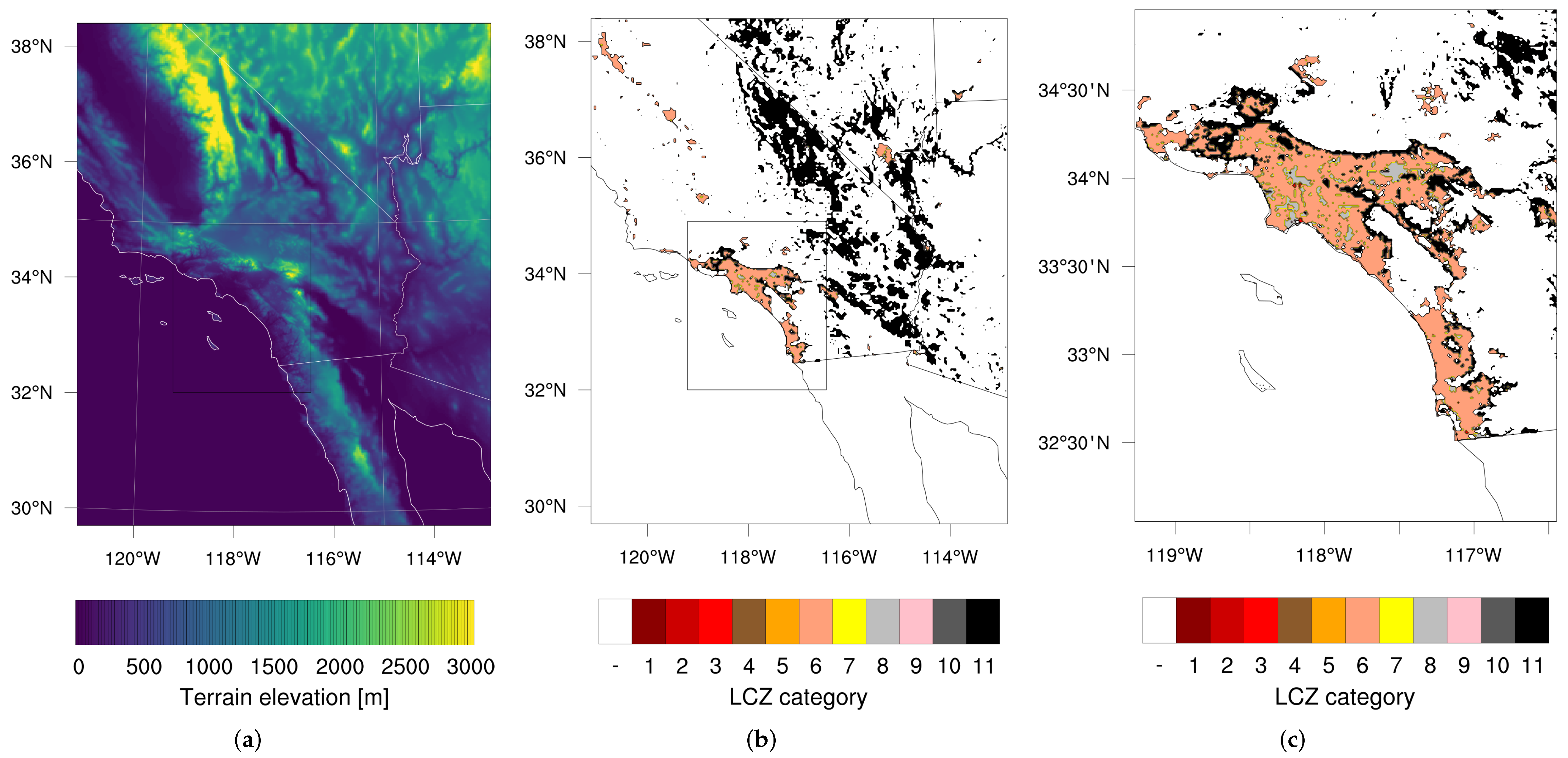
2. Configuration and Methods
3. Results and Discussion
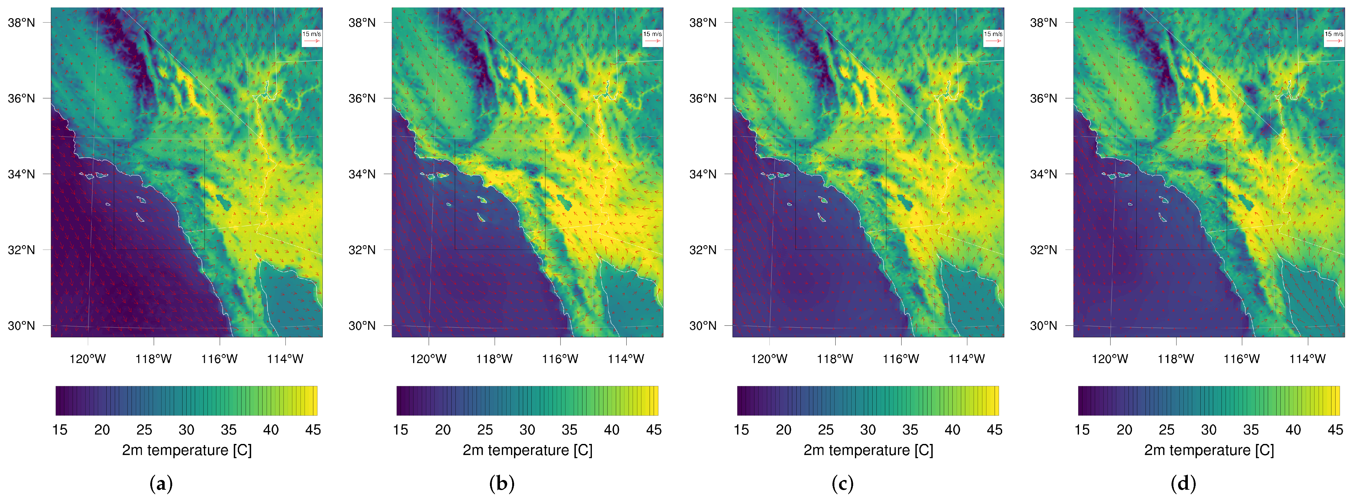
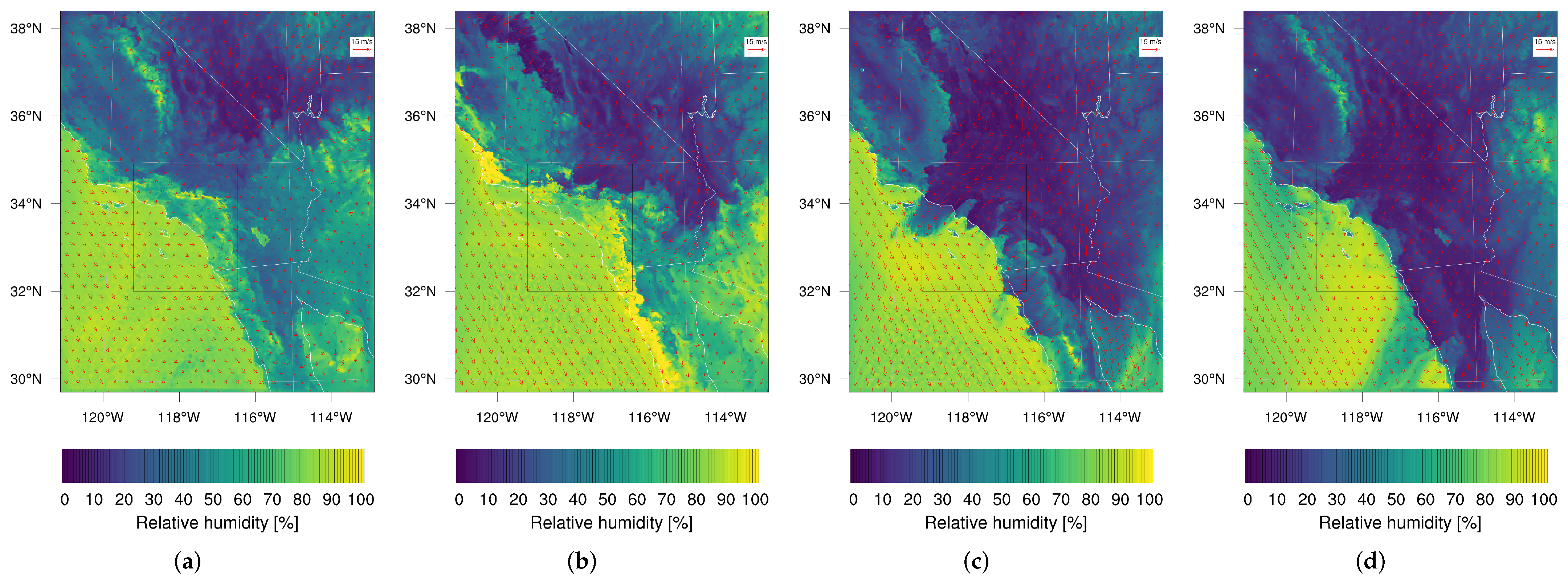
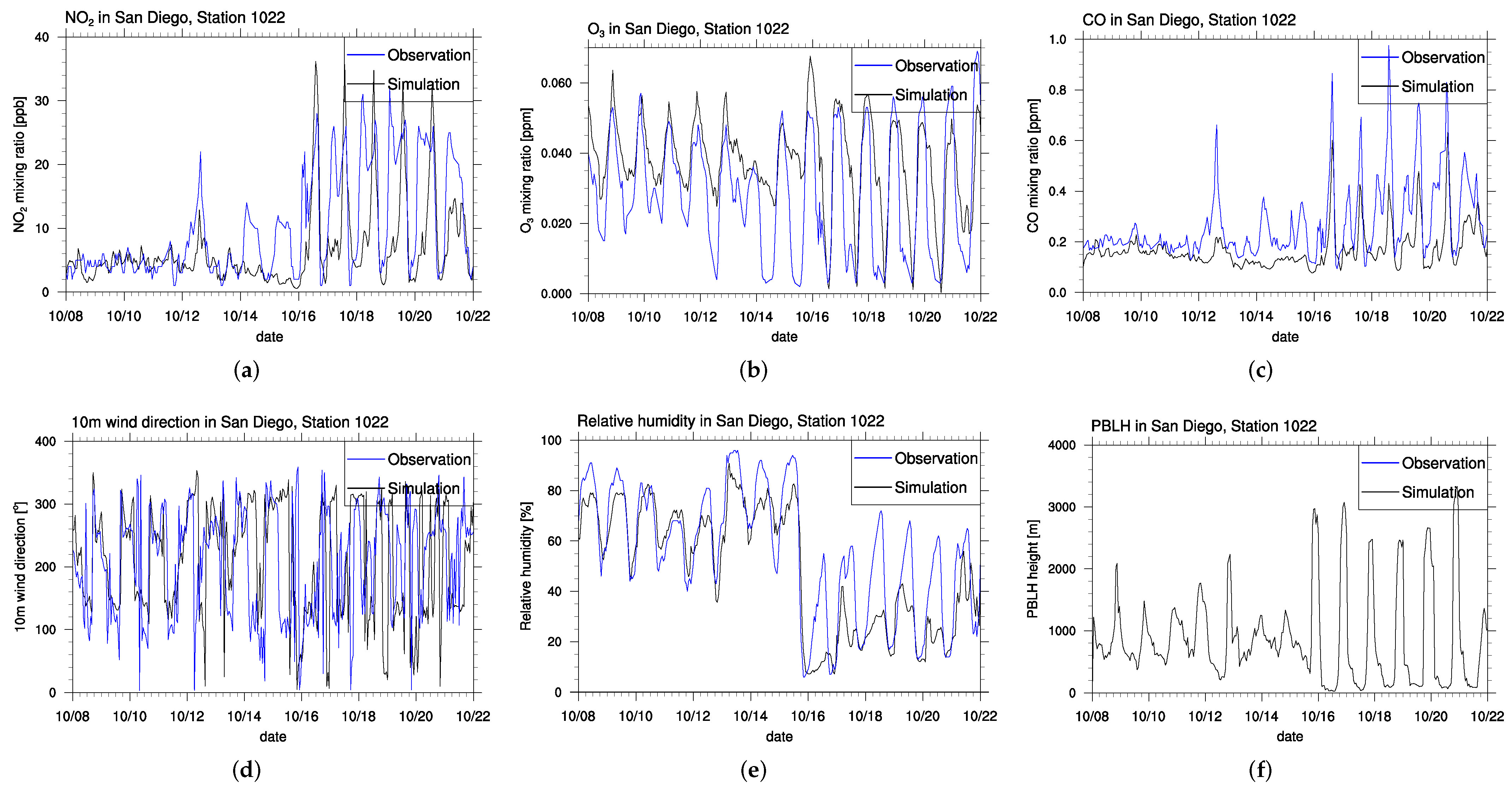
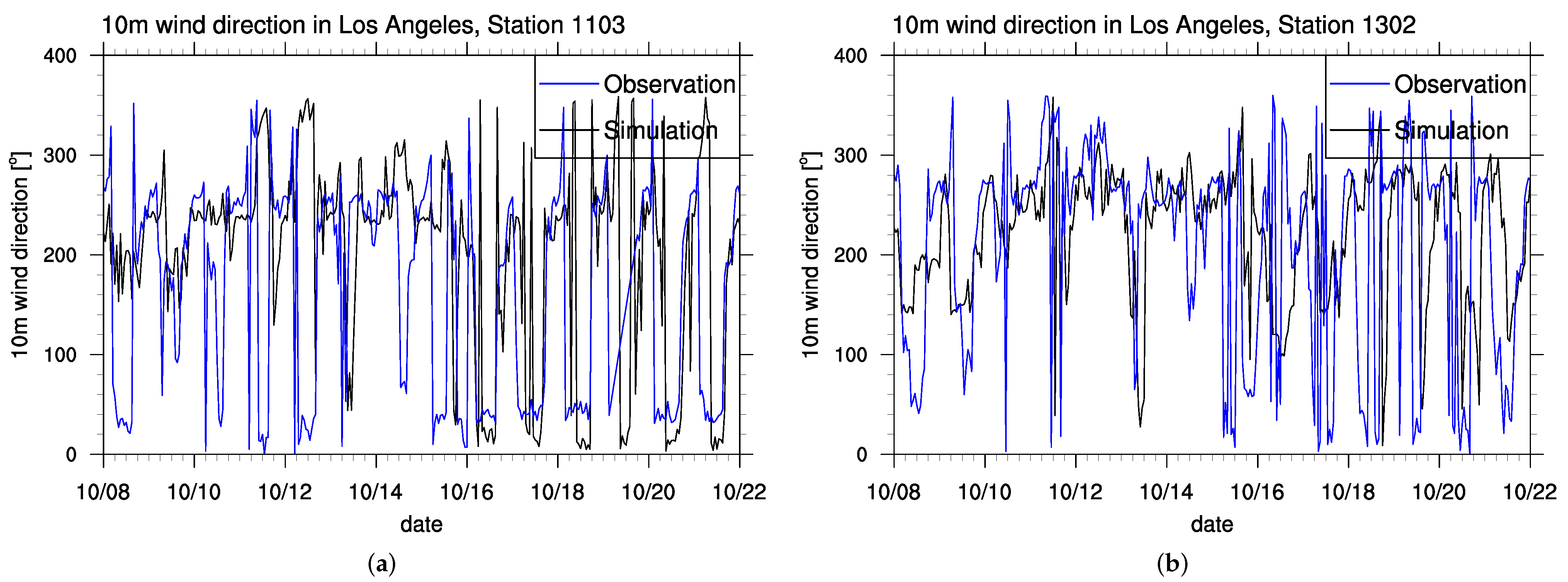
3.1. Meteorology
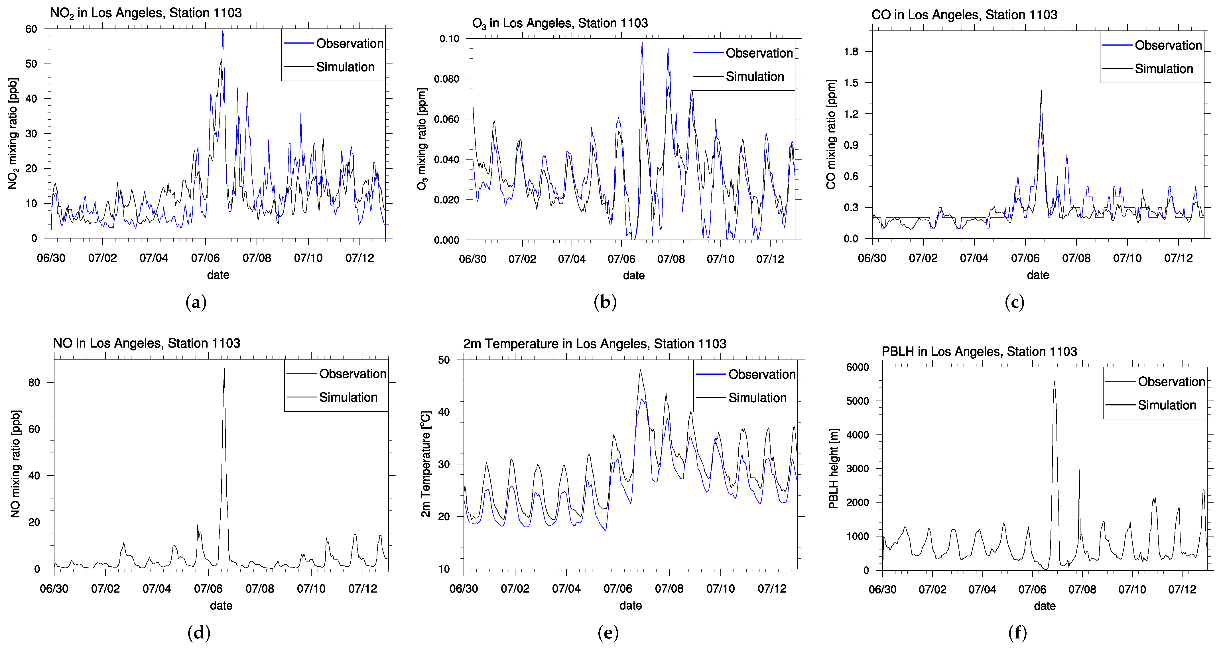
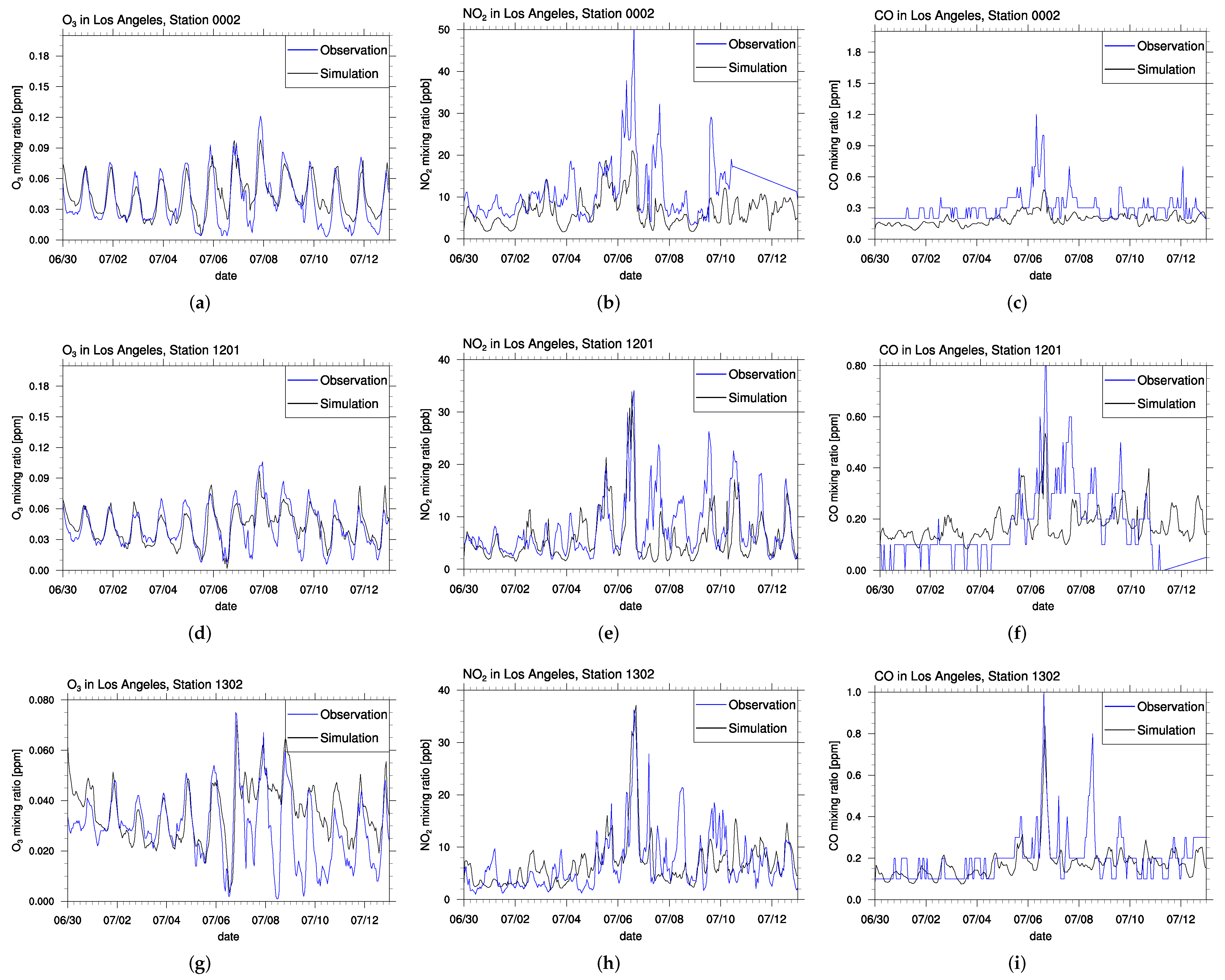
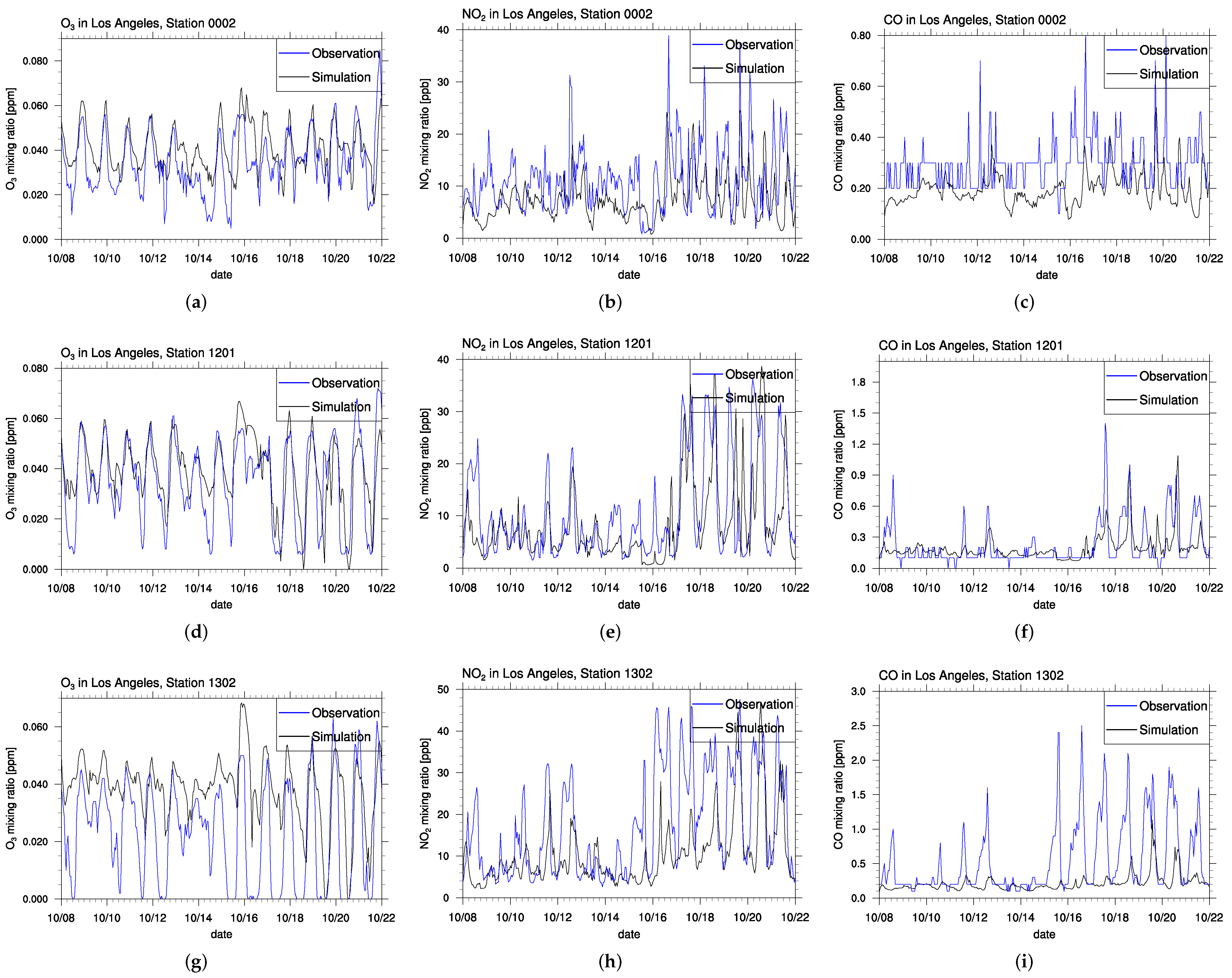
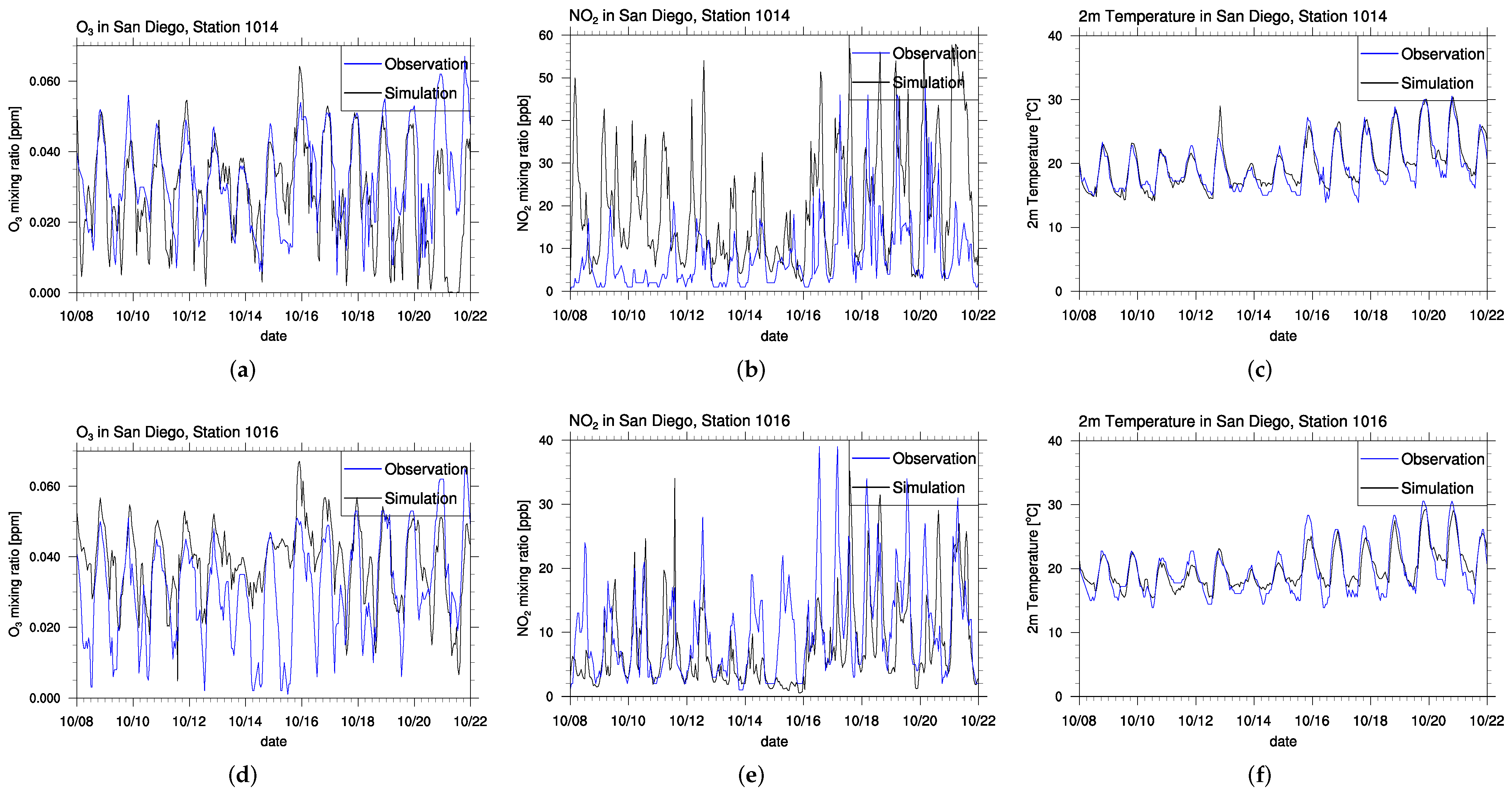
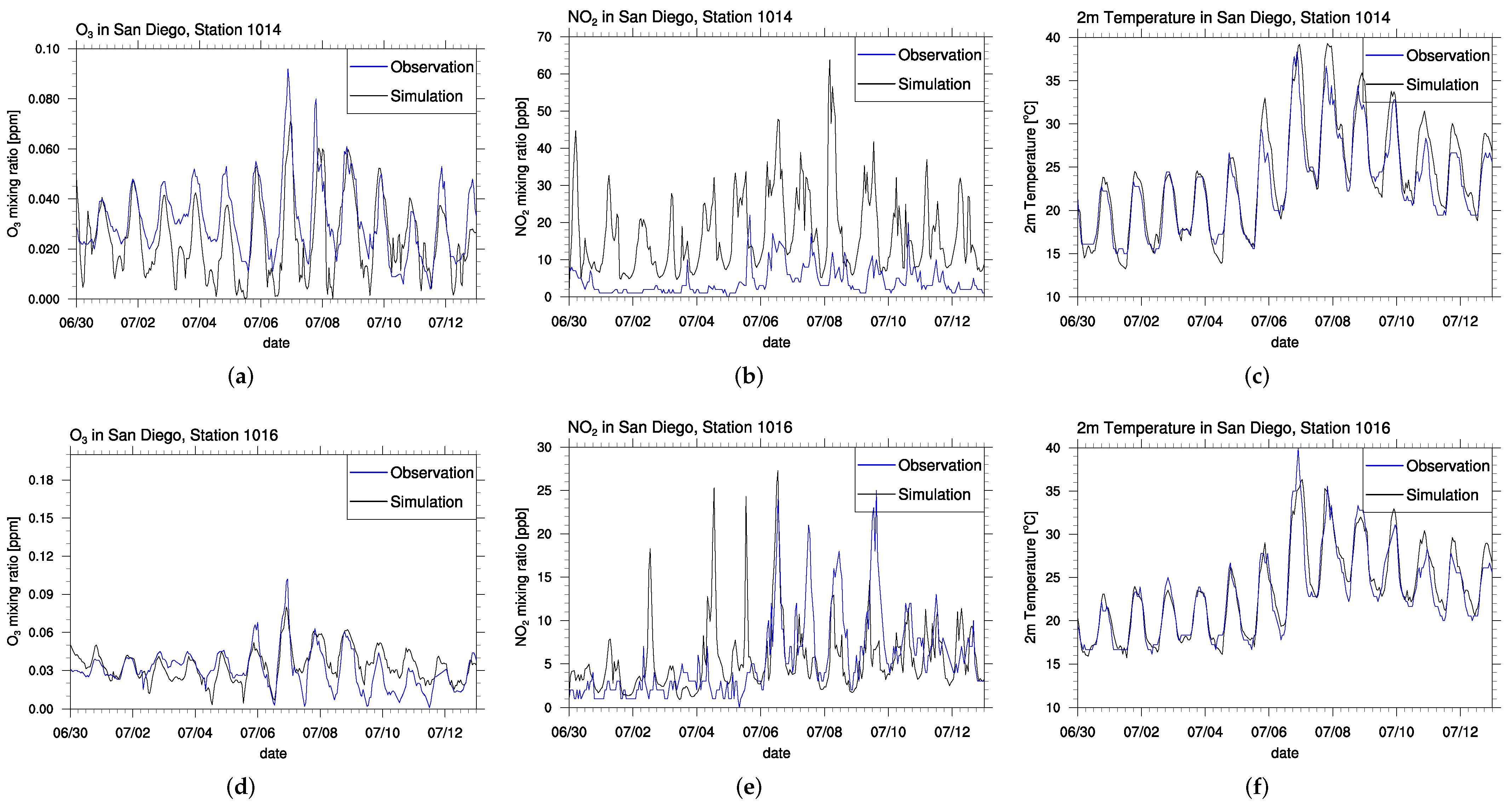
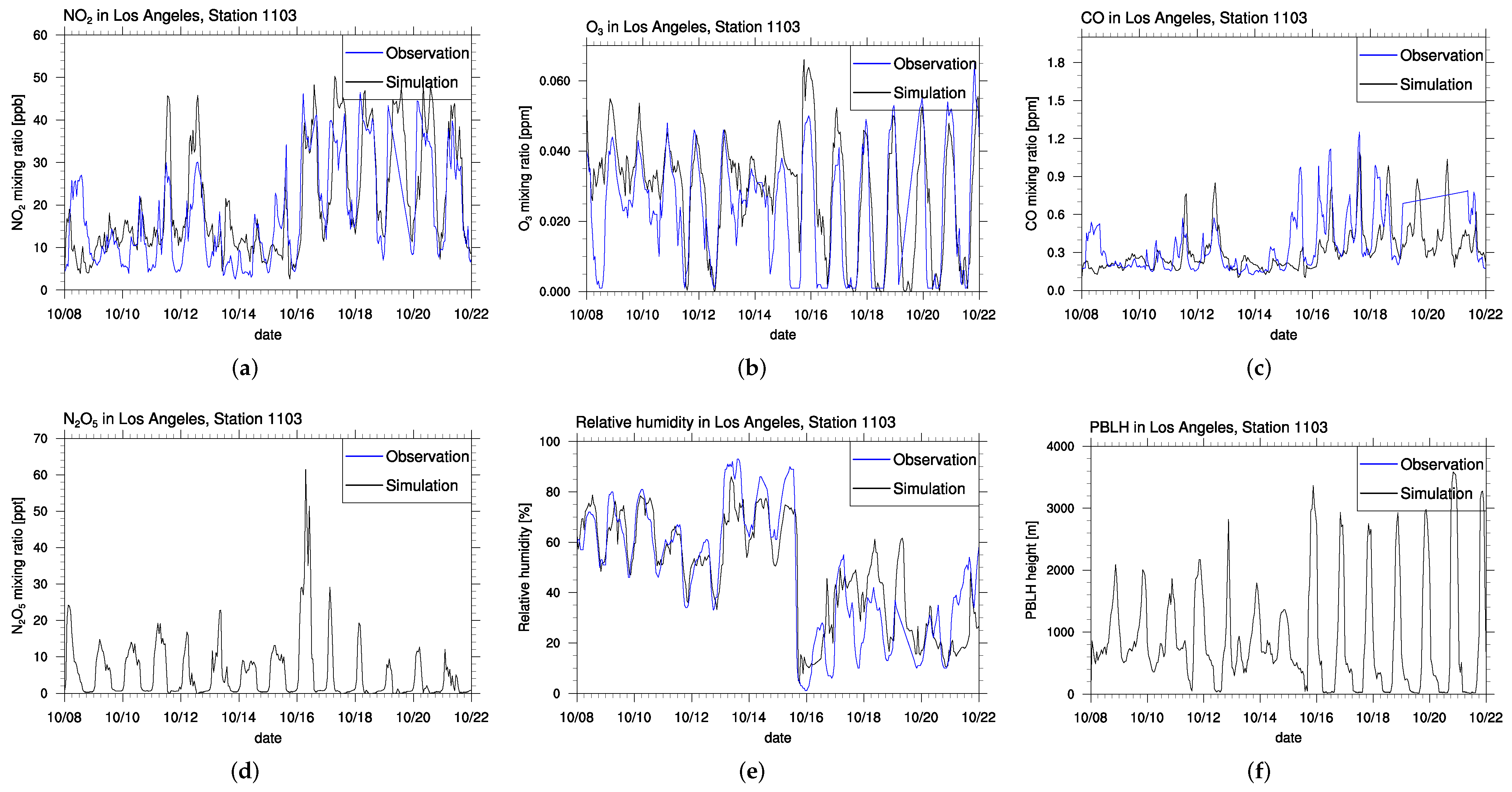
3.2. Comparison of Simulated O, CO, and NO Mixing Ratios with Observations
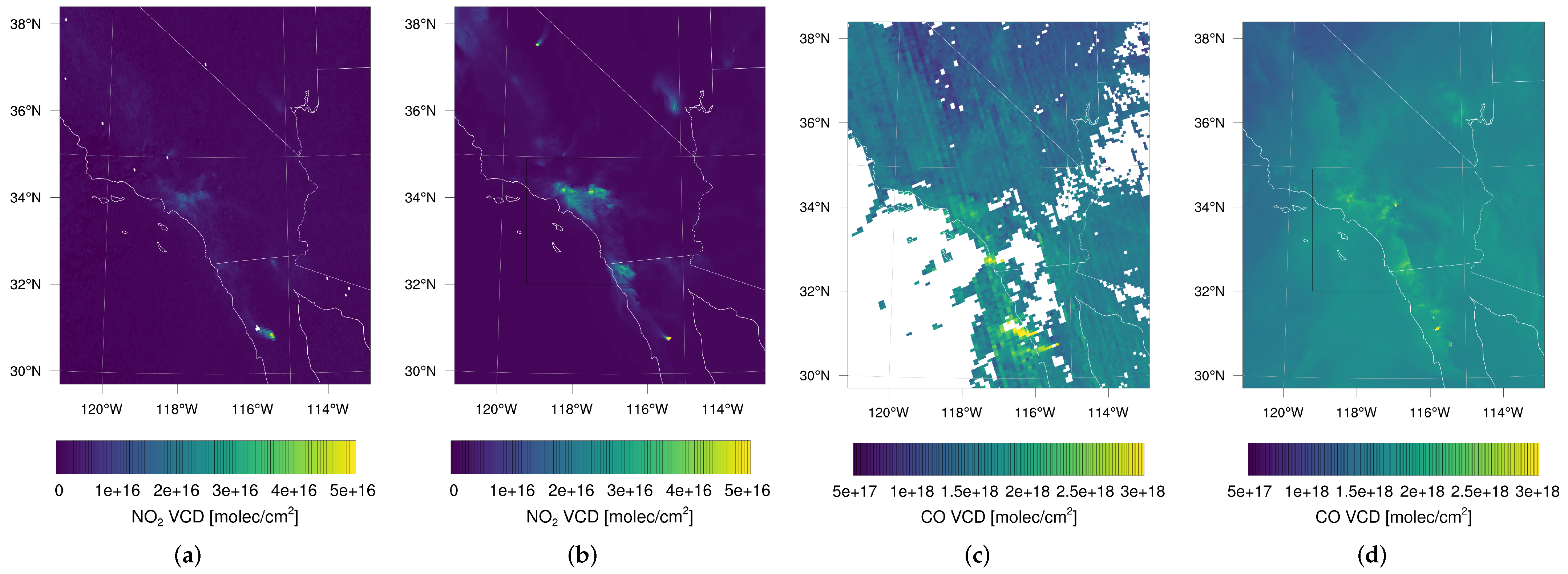
3.3. Comparison of Simulations and TROPOMI VCDs
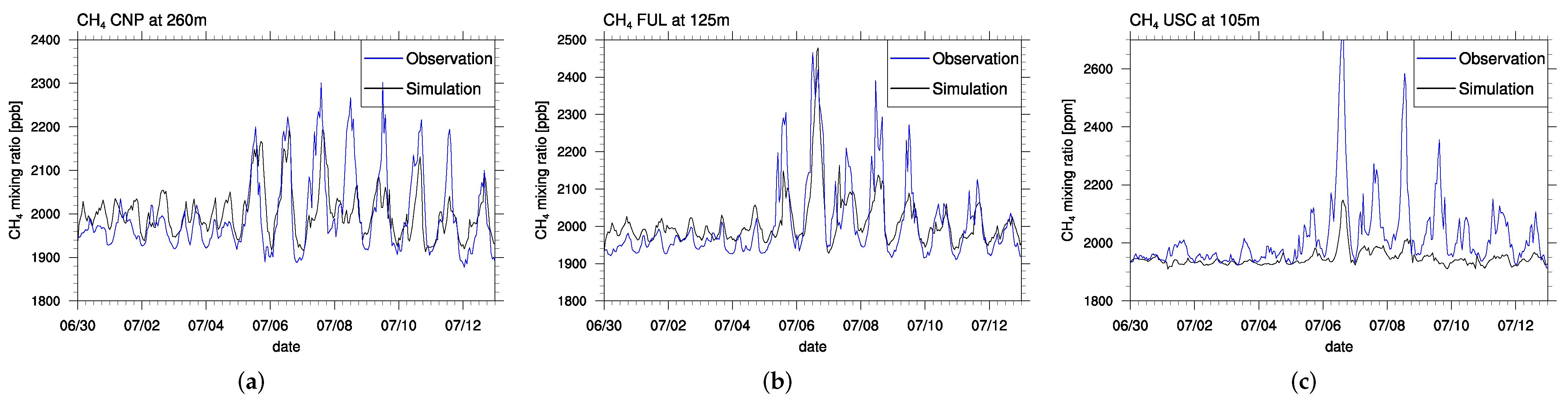
3.4. Comparison of Modeled and Observed Methane Mixing Ratios
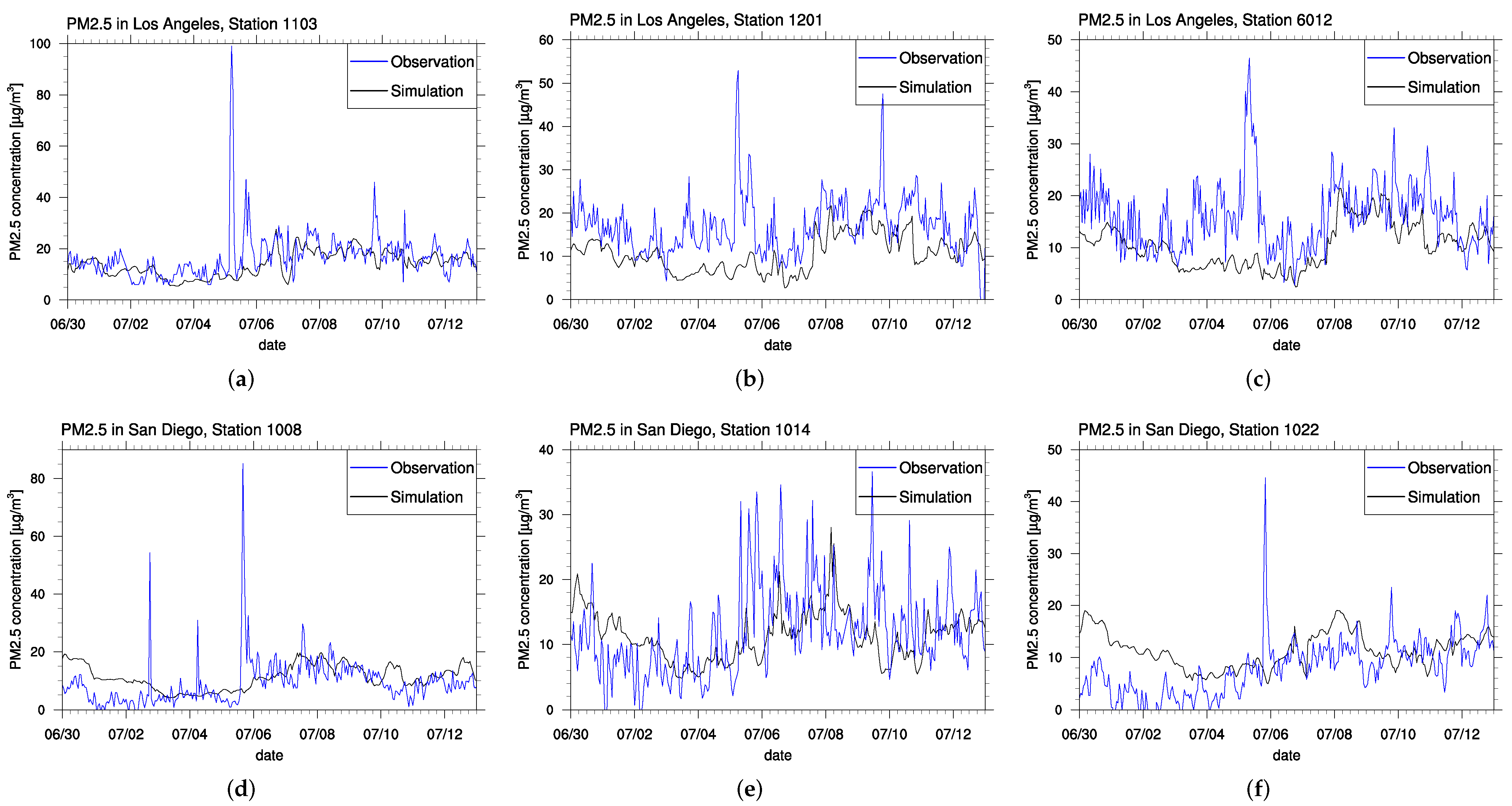
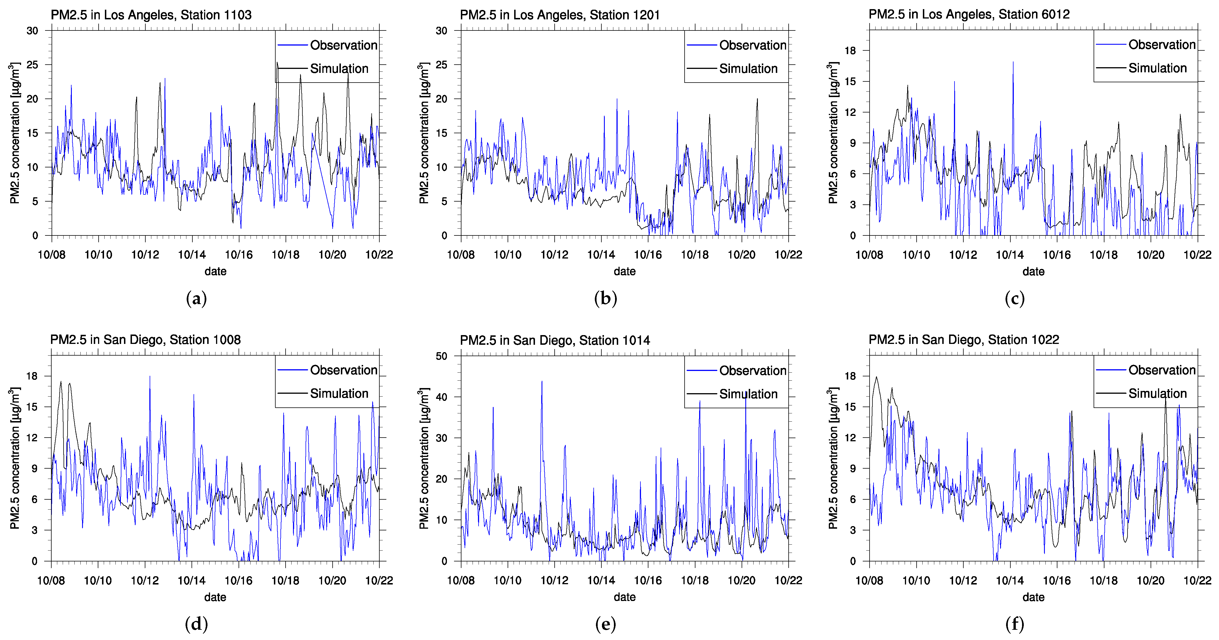
3.5. Comparison of Simulated and Observed PM2.5 Concentrations
4. Summary and Conclusions
Author Contributions
Funding
Institutional Review Board Statement
Informed Consent Statement
Data Availability Statement
Acknowledgments
Conflicts of Interest
References
- South Coast Air Quality Management District Ozone Season and Wildfire Impacts. 2020. Available online: http://www.aqmd.gov/docs/default-source/Agendas/Governing-Board/2020/2020-nov6-025.pdf?sfvrsn=2 (accessed on 21 February 2022).
- Nuvolone, D.; Petri, D.; Voller, F. The effects of ozone on human health. Environ. Sci. Pollut. Res. 2018, 25, 8074–8088. [Google Scholar] [CrossRef]
- Nussbaumer, C.M.; Cohen, R.C. The Role of Temperature and NOx in Ozone Trends in the Los Angeles Basin. Environ. Sci. Technol. 2020, 54, 15652–15659. [Google Scholar] [CrossRef]
- Hesterberg, T.W.; Bunn, W.B.; McClellan, R.O.; Hamade, A.K.; Long, C.M.; Valberg, P.A. Critical review of the human data on short-term nitrogen dioxide (NO2) exposures: Evidence for NO2 no-effect levels. Crit. Rev. Toxicol. 2009, 39, 743–781. [Google Scholar] [CrossRef]
- Pope, C.A., III; Dockery, D.W. Health effects of fine particulate air pollution: Lines that connect. J. Air Waste Manag. Assoc. 2006, 56, 709–742. [Google Scholar] [CrossRef]
- Nussbaumer, C.M.; Cohen, R.C. Impact of OA on the Temperature Dependence of PM2.5 in the Los Angeles Basin. Environ. Sci. Technol. 2021, 55, 3549–3558. [Google Scholar] [CrossRef]
- Moran, D.; Kanemoto, K.; Jiborn, M.; Wood, R.; Többen, J.; Seto, K.C. Carbon footprints of 13,000 cities. Environ. Res. Lett. 2018, 13, 064041. [Google Scholar] [CrossRef]
- Pachauri, R.K.; Allen, M.R.; Barros, V.R.; Broome, J.; Cramer, W.; Christ, R.; Church, J.A.; Clarke, L.; Dahe, Q.; Dasgupta, P.; et al. Climate Change 2014: Synthesis Report. Contribution of Working Groups I, II and III to the Fifth Assessment Report of the Intergovernmental Panel on Climate Change; IPCC: Geneva, Switzerland, 2014. [Google Scholar]
- Verhulst, K.; Karion, A.; Kim, J.; Salameh, P.; Sloop, C.; Keeling, R.; Weiss, R.; Duren, R.; Miller, J. In Situ Carbon Dioxide and Methane Measurements from the Los Angeles Megacity Carbon Project. Atmos. Chem. Phys. 2017, 17, 8313–8341. [Google Scholar] [CrossRef] [Green Version]
- Hedelius, J.K.; Feng, S.; Roehl, C.M.; Wunch, D.; Hillyard, P.W.; Podolske, J.R.; Iraci, L.T.; Patarasuk, R.; Rao, P.; O’Keeffe, D.; et al. Emissions and topographic effects on column CO2 (XCO2) variations, with a focus on the Southern California Megacity. J. Geophys. Res. Atmos. 2017, 122, 7200–7215. [Google Scholar] [CrossRef]
- Miller, J.B.; Lehman, S.J.; Verhulst, K.R.; Miller, C.E.; Duren, R.M.; Yadav, V.; Newman, S.; Sloop, C.D. Large and seasonally varying biospheric CO2 fluxes in the Los Angeles megacity revealed by atmospheric radiocarbon. Proc. Natl. Acad. Sci. USA 2020, 117, 26681–26687. [Google Scholar] [CrossRef]
- Duren, R.M.; Thorpe, A.K.; Foster, K.T.; Rafiq, T.; Hopkins, F.M.; Yadav, V.; Bue, B.D.; Thompson, D.R.; Conley, S.; Colombi, N.K.; et al. California’s methane super-emitters. Nature 2019, 575, 180–184. [Google Scholar] [CrossRef] [Green Version]
- Yadav, V.; Duren, R.; Mueller, K.; Verhulst, K.R.; Nehrkorn, T.; Kim, J.; Weiss, R.F.; Keeling, R.; Sander, S.; Fischer, M.L.; et al. Spatio-temporally Resolved Methane Fluxes From the Los Angeles Megacity. J. Geophys. Res. Atmos. 2019, 124, 5131–5148. [Google Scholar] [CrossRef] [Green Version]
- Ware, J.; Kort, E.A.; Duren, R.; Mueller, K.L.; Verhulst, K.; Yadav, V. Detecting Urban Emissions Changes and Events With a Near-Real-Time-Capable Inversion System. J. Geophys. Res. Atmos. 2019, 124, 5117–5130. [Google Scholar] [CrossRef]
- Zeng, Z.C.; Wang, Y.; Pongetti, T.J.; Gong, F.Y.; Newman, S.; Li, Y.; Natraj, V.; Shia, R.L.; Yung, Y.L.; Sander, S.P. Tracking the atmospheric pulse of a North American megacity from a mountaintop remote sensing observatory. Remote Sens. Environ. 2020, 248, 112000. [Google Scholar] [CrossRef]
- Parrish, D.D.; Xu, J.; Croes, B.; Shao, M. Air quality improvement in Los Angeles—Perspectives for developing cities. Front. Environ. Sci. Eng. 2016, 10, 11. [Google Scholar] [CrossRef]
- Stewart, D.R.; Saunders, E.; Perea, R.A.; Fitzgerald, R.; Campbell, D.E.; Stockwell, W.R. Linking air quality and human health effects models: An application to the Los Angeles air basin. Environ. Health Insights 2017, 11, 1178630217737551. [Google Scholar] [CrossRef] [Green Version]
- Connerton, P.; Vicente de Assunção, J.; Maura de Miranda, R.; Dorothée Slovic, A.; José Pérez-Martínez, P.; Ribeiro, H. Air Quality during COVID-19 in Four Megacities: Lessons and Challenges for Public Health. Int. J. Environ. Res. Public Health 2020, 17, 5067. [Google Scholar] [CrossRef]
- Pan, S.; Jung, J.; Li, Z.; Hou, X.; Roy, A.; Choi, Y.; Gao, H.O. Air Quality Implications of COVID-19 in California. Sustainability 2020, 12, 7067. [Google Scholar] [CrossRef]
- Grell, G.A.; Peckham, S.E.; Schmitz, R.; McKeen, S.A.; Frost, G.; Skamarock, W.C.; Eder, B. Fully coupled “online” chemistry within the WRF model. Atmos. Environ. 2005, 39, 6957–6975. [Google Scholar] [CrossRef]
- Fast, J.D.; Gustafson, W.I., Jr.; Easter, R.C.; Zaveri, R.A.; Barnard, J.C.; Chapman, E.G.; Grell, G.A.; Peckham, S.E. Evolution of ozone, particulates, and aerosol direct radiative forcing in the vicinity of Houston using a fully coupled meteorology-chemistry-aerosol model. J. Geophys. Res. Atmos. 2006, 111. [Google Scholar] [CrossRef]
- Skamarock, W.C.; Klemp, J.B.; Dudhia, J.; Gill, D.O.; Barker, D.M.; Wang, W.; Powers, J.G. A Description of the Advanced Research WRF Version 3. NCAR Technical Note-475+ STR. 2008. Available online: https://opensky.ucar.edu/islandora/object/technotes:500 (accessed on 18 January 2022).
- Kim, J.; Verhulst, K.; Lueker, T.; Salameh, P.; Cox, A.; Walker, S.; Paplawsky, B.; Prinzivalli, S.; Fain, C.; Stock, M.; et al. In Situ Carbon Dioxide, Methane, and Carbon Monoxide Mole Fractions from the Los Angeles Megacity Carbon Project; Technical Report; National Institute of Standards and Technology: Gaithersburg, MD, USA, 2021. [CrossRef]
- ESA; CSP. TROPOMI Level 2 Carbon Monoxide Total Column Products; Technical Report; European Space Agency: Paris, France, 2021. [Google Scholar] [CrossRef]
- ESA; CSP. TROPOMI Level 2 Nitrogen Dioxide Tropospheric Column Products; Technical Report; European Space Agency: Paris, France, 2021. [Google Scholar] [CrossRef]
- EPA. Pre-Generated Data Files. 2022. Available online: https://aqs.epa.gov/aqsweb/airdata/download_files.html (accessed on 18 January 2022).
- Emmons, L.K.; Schwantes, R.H.; Orlando, J.J.; Tyndall, G.; Kinnison, D.; Lamarque, J.F.; Marsh, D.; Mills, M.J.; Tilmes, S.; Bardeen, C.; et al. The Chemistry Mechanism in the Community Earth System Model Version 2 (CESM2). J. Adv. Model. Earth Syst. 2020, 12, e2019MS001882. [Google Scholar] [CrossRef] [Green Version]
- Stewart, I.D.; Oke, T.R. Local Climate Zones for Urban Temperature Studies. Bull. Am. Meteorol. Soc. 2012, 93, 1879–1900. [Google Scholar] [CrossRef]
- Martilli, A.; Clappier, A.; Rotach, M.W. An urban surface exchange parameterisation for mesoscale models. Bound.-Layer Meteorol. 2002, 104, 261–304. [Google Scholar] [CrossRef]
- Salamanca, F.; Martilli, A. A new Building Energy Model coupled with an Urban Canopy Parameterization for urban climate simulations-part II. Validation with one dimension off-line simulations. Theorectical Appl. Climatol. 2010, 99, 345–356. [Google Scholar] [CrossRef]
- Iacono, M.J.; Delamere, J.S.; Mlawer, E.J.; Shephard, M.W.; Clough, S.A.; Collins, W.D. Radiative forcing by long-lived greenhouse gases: Calculations with the AER radiative transfer models. J. Geophys. Res. Atmos. 2008, 113. [Google Scholar] [CrossRef]
- Hong, S.Y.; Lim, J.O.J. The WRF single-moment 6-class microphysics scheme (WSM6). Asia-Pac. J. Atmos. Sci. 2006, 42, 129–151. [Google Scholar]
- Niu, G.Y.; Yang, Z.L.; Mitchell, K.E.; Chen, F.; Ek, M.B.; Barlage, M.; Kumar, A.; Manning, K.; Niyogi, D.; Rosero, E.; et al. The community Noah land surface model with multiparameterization options (Noah-MP): 1. Model description and evaluation with local-scale measurements. J. Geophys. Res. Atmos. 2011, 116. [Google Scholar] [CrossRef] [Green Version]
- Janjić, Z. The surface layer in the NCEP Eta Model. In Proceedings of the Eleventh Conference on Numerical Weather Prediction, Norfolk, VA, USA, 19–23 August 1996; pp. 19–23. [Google Scholar]
- Bougeault, P.; Lacarrere, P. Parameterization of orography-induced turbulence in a mesobeta—Scale model. Mon. Weather Rev. 1989, 117, 1872–1890. [Google Scholar] [CrossRef]
- Hersbach, H.; Bell, B.; Berrisford, P.; Hirahara, S.; Horányi, A.; Muñoz-Sabater, J.; Nicolas, J.; Peubey, C.; Radu, R.; Schepers, D. The ERA5 global reanalysis. Q. J. R. Meteorol. Soc. 2020, 146, 1999–2049. [Google Scholar] [CrossRef]
- Buchholz, R.R.; Emmons, L.K.; Tilmes, S.; TCD Team. CAM-Chem Output for Boundary Conditions. Technical Report. UCAR/NCAR Lat: 0 to 90. Lon: 0 to 360, February–May 2019. 2021. Available online: https://wiki.ucar.edu/pages/viewpage.action?pageId=372834733 (accessed on 18 January 2022).
- Huang, B.; Liu, C.; Banzon, V.; Freeman, E.; Graham, G.; Hankins, B.; Smith, T.; Zhang, H.M. Improvements of the Daily Optimum Interpolation Sea Surface Temperature (DOISST) Version 2.1. J. Clim. 2021, 34, 2923–2939. [Google Scholar] [CrossRef]
- Chin, M.; Ginoux, P.; Kinne, S.; Torres, O.; Holben, B.N.; Duncan, B.N.; Martin, R.V.; Logan, J.A.; Higurashi, A.; Nakajima, T. Tropospheric aerosol optical thickness from the GOCART model and comparisons with satellite and Sun photometer measurements. J. Atmos. Sci. 2002, 59, 461–483. [Google Scholar] [CrossRef]
- Madronich, S.; Flocke, S.; Zeng, J.; Petropavlovskikh, I.; Lee-Taylor, J. Tropospheric Ultraviolet-Visible Model (TUV) version 4.1. Natl. Cent. Atmos. Res. 2002, 3000. [Google Scholar]
- Janssens-Maenhout, G.; Dentener, F.; Van Aardenne, J.; Monni, S.; Pagliari, V.; Orlandini, L.; Klimont, Z.; Kurokawa, J.i.; Akimoto, H.; Ohara, T.; et al. EDGAR-HTAP: A Harmonized Gridded Air Pollution Emission Dataset Based on National Inventories; JRC68434, EUR Report No EUR; European Commission Publications Office: Ispra, Italy, 2012; Volume 25, pp. 299–2012. [Google Scholar]
- Guenther, A.; Karl, T.; Harley, P.; Wiedinmyer, C.; Palmer, P.I.; Geron, C. Estimates of global terrestrial isoprene emissions using MEGAN (Model of Emissions of Gases and Aerosols from Nature). Atmos. Chem. Phys. 2006, 6, 3181–3210. [Google Scholar] [CrossRef] [Green Version]
- Wiedinmyer, C.; Akagi, S.K.; Yokelson, R.J.; Emmons, L.K.; Al-Saadi, J.A.; Orlando, J.J.; Soja, A.J. The Fire INventory from NCAR (FINN): A high resolution global model to estimate the emissions from open burning. Geosci. Model Dev. 2011, 4, 625–641. [Google Scholar] [CrossRef] [Green Version]
- Demuzere, M.; Hankey, S.; Mills, G.; Zhang, W.; Lu, T.; Bechtel, B. Combining expert and crowd-sourced training data to map urban form and functions for the continental US. Sci. Data 2020, 7, 264. [Google Scholar] [CrossRef]
- Wesely, M. Parameterization of surface resistances to gaseous dry deposition in regional-scale numerical models. Atmos. Environ. 1989, 23, 1293–1304. [Google Scholar] [CrossRef]


| Parameter | Setting |
|---|---|
| Longwave radiation | LW RRTMG scheme [31] |
| Shortwave radiation | SW RRTMG scheme [31] |
| Microphysics | WSM 6-class graupel scheme [32] |
| Land-surface model | Noah Land-Surface Model [33] |
| Surface-layer model | Monin–Obukhov Similarity scheme [34] |
| Boundary-layer model | Bougeault and Lacarrere (BouLac) [35] |
| Cumulus parameterization | Not needed due to high model resolution |
| Urban parameterization | BEP+BEM [29,30] |
| Initial and boundary data | ERA-5 [36], CAM-CHEM [37] |
| Sea surface temperature data | Optimum Interpolation SST v2.1 [38] |
| Time step | 15 and 5 s (domain 1 and 2) |
| Simulated time range | 30 June 2018–13 July 2018 |
| 8 October 2018–22 October 2018 | |
| Nudging | For the first week, see text |
| Horizontal resolution | 3 and 1 km (domain 1 and 2) |
| Longitude and latitude | 268 × 325 horizontal grid cells (both domains) |
| Vertical grid size | 60 levels |
| Vertical size of the first cell | ≈5 m |
| Pressure at top boundary | 50 hPa |
| Chemistry mechanism | MOZART-T1 [27] |
| Aerosols | GOCART [39] |
| Photolysis scheme | Updated TUV [40] |
| Emissions | 2017 National Emissions Inventory [41] |
| Bioemissions | MEGAN [42] |
| Wildfire emissions | FINN [43] |
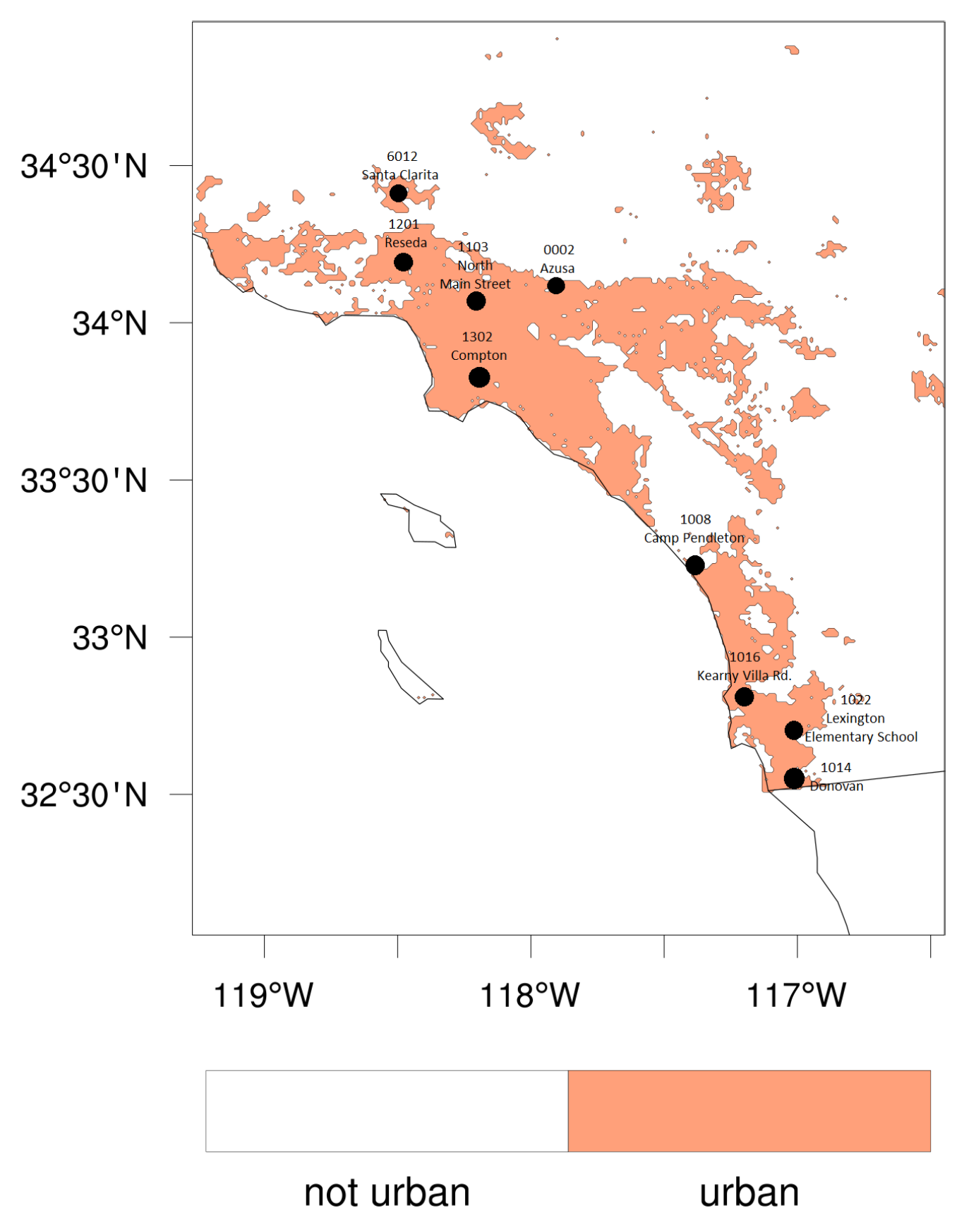
| County | Station Number | Station Name |
|---|---|---|
| Los Angeles | 0002 | Azusa |
| Los Angeles | 1103 | North Main Street |
| Los Angeles | 1201 | Reseda |
| Los Angeles | 1302 | Compton |
| Los Angeles | 6012 | Santa Clarita |
| San Diego | 1008 | Camp Pendleton |
| San Diego | 1014 | Donovan |
| San Diego | 1016 | Kearny Villa Road |
| San Diego | 1022 | Lexington Elementary School |
| Station | Species | Correlation R | Mean Bias | RMSE |
|---|---|---|---|---|
| LA Azusa | O | 0.85 | 0.0047 ppm | 0.014 ppm |
| LA Azusa | NO | 0.62 | −5.2 ppb | 7.4 ppb |
| LA Azusa | CO | 0.60 | −0.11 ppm | 0.16 ppm |
| LA North Main Street | O | 0.77 | 0.0024 ppm | 0.012 ppm |
| LA North Main Street | NO | 0.65 | −0.27 ppb | 7.3 ppb |
| LA North Main Street | CO | 0.76 | −0.022 ppm | 0.11 ppm |
| LA Reseda | O | 0.8 | 0.00049 ppm | 0.012 ppm |
| LA Reseda | NO | 0.63 | −1.9 ppb | 5.0 ppb |
| LA Reseda | CO | 0.45 | 0.024 ppm | 0.13 ppm |
| LA Compton | O | 0.6 | 0.0068 ppm | 0.013 ppm |
| LA Compton | NO | 0.64 | 0.080 ppb | 4.5 ppb |
| LA Compton | CO | 0.63 | −0.026 ppm | 0.10 ppm |
| SD Donovan | O | 0.74 | −0.0074 ppm | 0.013 ppm |
| SD Donovan | NO | 0.35 | 13 ppb | 16 ppb |
| SD Kearny Villa Road | O | 0.68 | 0.0035 ppm | 0.012 ppm |
| SD Kearny Villa Road | NO | 0.37 | −0.057 ppb | 4.9 ppb |
| SD Lexington Elementary School | O | 0.79 | 0.0023 ppm | 0.011 ppm |
| SD Lexington Elementary School | NO | 0.56 | 1.3 ppb | 3.7 ppb |
| SD Lexington Elementary School | CO | 0.71 | −0.076 ppm | 0.10 ppm |
| Station | Species | Correlation R | Mean Bias | RMSE |
|---|---|---|---|---|
| LA Azusa | O | 0.61 | 0.0061 ppm | 0.012 ppm |
| LA Azusa | NO | 0.40 | −3.7 ppb | 7.1 ppb |
| LA Azusa | CO | 0.26 | −0.10 ppm | 0.14 ppm |
| LA North Main Street | O | 0.71 | 0.0051 ppm | 0.013 ppm |
| LA North Main Street | NO | 0.76 | 2.0 ppb | 8.8 ppb |
| LA North Main Street | CO | 0.59 | −0.091 ppm | 0.22 ppm |
| LA Reseda | O | 0.75 | 0.0040 ppm | 0.012 ppm |
| LA Reseda | NO | 0.61 | −2.0 ppb | 7.8 ppb |
| LA Reseda | CO | 0.54 | −0.026 ppm | 0.18 ppm |
| LA Compton | O | 0.56 | 0.016 ppm | 0.021 ppm |
| LA Compton | NO | 0.55 | −6.9 ppb | 12 ppb |
| LA Compton | CO | 0.31 | −0.33 ppm | 0.59 ppm |
| SD Donovan | O | 0.55 | −0.0043 ppm | 0.014 ppm |
| SD Donovan | NO | 0.40 | 12 ppb | 18 ppb |
| SD Kearny Villa Road | O | 0.54 | 0.0079 ppm | 0.015 ppm |
| SD Kearny Villa Road | NO | 0.50 | −2.5 ppb | 7.7 ppb |
| SD Lexington Elementary School | O | 0.037 | 0.0095 ppm | 0.015 ppm |
| SD Lexington Elementary School | NO | 0.63 | −3.3 ppb | 7.2 ppb |
| SD Lexington Elementary School | CO | 0.75 | −0.10 ppm | 0.14 ppm |
| Station | Correlation R | Mean Bias | RMSE |
|---|---|---|---|
| CNP | 0.62 | 3.3 ppb | 70 ppb |
| FUL | 0.81 | 2.3 ppb | 63 ppb |
| USC | 0.76 | −75 ppb | 129 ppb |
Publisher’s Note: MDPI stays neutral with regard to jurisdictional claims in published maps and institutional affiliations. |
© 2022 by the authors. Licensee MDPI, Basel, Switzerland. This article is an open access article distributed under the terms and conditions of the Creative Commons Attribution (CC BY) license (https://creativecommons.org/licenses/by/4.0/).
Share and Cite
Herrmann, M.; Gutheil, E. Simulation of the Air Quality in Southern California, USA in July and October of the Year 2018. Atmosphere 2022, 13, 548. https://doi.org/10.3390/atmos13040548
Herrmann M, Gutheil E. Simulation of the Air Quality in Southern California, USA in July and October of the Year 2018. Atmosphere. 2022; 13(4):548. https://doi.org/10.3390/atmos13040548
Chicago/Turabian StyleHerrmann, Maximilian, and Eva Gutheil. 2022. "Simulation of the Air Quality in Southern California, USA in July and October of the Year 2018" Atmosphere 13, no. 4: 548. https://doi.org/10.3390/atmos13040548
APA StyleHerrmann, M., & Gutheil, E. (2022). Simulation of the Air Quality in Southern California, USA in July and October of the Year 2018. Atmosphere, 13(4), 548. https://doi.org/10.3390/atmos13040548