Comparison between Puff and Lagrangian Particle Dispersion Models at a Complex and Coastal Site

Abstract

A comparison between a puff atmospheric dispersion model (hereafter: PuM) and a Lagrangian particle model (hereafter: LPM) was conducted for a real case of emissions from an industrial plant, in the context of a complex and coastal site. The PuM’s approach is well-known and widely adopted worldwide, thanks to the authoritative suggestions by the US-EPA for regulatory use as, according to the definitions included in its guidelines, an “alternative” to “preferred” models; LPMs are more advanced models and have gained reliability over the last two decades. Therefore, it is of interest to provide insights into the decision to adopt or recommend, in the field of atmospheric impact assessment, a more advanced, but more knowledge- and resource-intensive, modeling tool, rather than an established albeit less accurate one. An inter-comparison of the two approaches is proposed based on the use of various statistical and comparative parameters with the goal of studying their differences in reproducing maps of ground-level ambient concentration statistics for assessment purposes (annual means, hourly peaks). The models were tested under a year-long simulation. The dispersion from both a point and a volume source, belonging to an existing industrial plant, was analyzed separately. The inter-comparison was performed through the analysis of 2D ground concentration maps, scatterplots, and three classical indices from the 2D maps of annual concentration statistics. To correlate the differences among models with site characteristics, the statistics were analyzed not only globally, but also according to distance from the source, the elevation, and the land-use classification. The analysis shows that around-its-axis plume dispersion in LPM is lower than in PuM over all the land-use types except water surfaces, in agreement with the theoretical basis provided by the models. Because of its more advanced theoretical formulation, e.g., in the interaction of the plume with the complex terrain and the three-dimensional wind field, an LPM used as a comparison term allowed us to highlight the weaknesses of a more traditional approach, such as PuM, in reproducing effects such as plume up-sloping, deflection, channeling, confinement, and wind shear diffusion.

1. Introduction

Air pollution is a topic of great interest for the quality of human life; pollutants can be of natural or anthropogenic origin and can be essentially classified as reactive or non-reactive. The latter undergo no or scarce change once emitted (CO for example), while the former are formed or transformed through chemical reactions and physical phenomena involving precursors in the atmosphere (NO₂, SO₂, particulate matter, O₃).

Human exposure to airborne pollutants can lead to short- and long-term health effects, mainly to the respiratory and cardiovascular systems. Recently, in Italy, guidelines to harmonize atmospheric and sanitary impact assessment have been released by ISPRA, the national environmental protection agency (ISPRA, 2016), in the wake of the serious evidence of health problems found around a major steel plant in Taranto. In this report, to quantify the risk on population health, the not-negligible possibility of calculating or predicting air pollutant concentrations using dispersion models is emphasized.

In Italy, moreover, problematical dispersion situations are the norm, due to an almost ubiquitous climatic influence of the coast (Italy is the 15th country in the world per coastline length, with a coast/area ratio higher than countries such as Canada or Malaysia, [1]) and complex terrain (76.8% of Italian territory has an altitude >200 m above sea level, 35.2% >600 m, [2]).

Recently, annual simulations by a Lagrangian particle model (hereafter: LPM) (the model SPRAY described below, [3]) supported an air quality assessment study for an industrial plant at an Italian complex and coastal site. Thanks to the availability of the associated database, the comparison of a puff atmospheric dispersion model (hereafter: PuM) with this modeling approach was performed through various statistical comparative parameters.

Both approaches have gradually established themselves in their proper ambits of application after several studies of comparison with experimental data, in which they proved sufficient performance scores with respect to acceptance criteria. Within these acceptance criteria, which are global and rather broad, important differences can be hidden between models of different complexity in describing atmospheric dispersion phenomena in particular situations of complex and inhomogeneous terrain.

Unfortunately, a complementary comparison with experimental data is not possible in most real cases since it is not always possible to have available or to implement a complete monitoring network to cover all situations in the territory. However, the lack of adequate experimental validation of the results does not preclude the normal use of dispersion model simulations as an important element of assessing the impact of anthropogenic activity and, ultimately, its performance even on terrain as complex as that examined here.

Several publications exist comparing the two approaches, both with (for example: [4,5,6]) and without pertinent experimental data (for example: [7,8,9,10]). According to these studies, at the mesoscale or in the far-field ([4]) the two approaches lead to more comparable results, at the local scale or in the near field greater differences emerge [5,6,7,8,9,10]. The novelty of this study is that we systematically compared the long-term statistics (averages, maxima) of the hourly concentration calculated over the whole domain in a real case, thus considering many aspects of the particularly varied context (very complex terrain near the coastline, the presence of different types of land use, and the proximity of the industrial plant to inhabited areas).

The site examined is rich in heterogeneous and complex local situations. This achieved the goal of bringing out important differences in results from the two approaches. In the final analysis, the objective is therefore also to help those who have the important task of assessing the atmospheric impact of a pollution source, to choose the most suitable dispersion model for the situation under investigation and its most appropriate options, and also to interpret the results in light of the chosen model.

The two approaches have been used independently, according to the specific competencies, by the University of Genoa—which adopted CALPUFF, a PuM—and ARIANET—which adopted SPRAY, an LPM. Finally, the results of parallel simulations run in the same annual 3D meteorological situations were compared. The objective was to study the different behaviors in reproducing maps of environmental concentration statistics for assessment purposes (annual averages, maxima, and percentiles) and showing if, when, and where these differences are significant.

Dispersion was considered separately from a hot elevated point source (stack of an oven) and a ground volume source at ambient temperature (covered storage area). The comparison was performed by means of numerous techniques, including the calculation of statistical indices such as Fractional Bias, the Index of Agreement, and Quantiles, as per many studies before (for example: [11,12], and the complete bibliography in their studies).

2. PuM and LPM

The two modeling approaches are referred to as “Lagrangian”. In this approach, the trajectory of a portion of a pollutant plume is not solved in the observer’s reference system, but in the reference system constrained to the portion of the plume itself. In the case of a PuM, the cloud of polluted air expands gradually with time according to the prescribed “expansion rate” and a Gaussian dispersion shape. In the LPM, independent solutions are given instead for a large portion of the points of the plume cross-section, the “particles”.

2.1. The PuM CALPUFF

The US-EPA’s Guideline on Air Quality Models (also published as Appendix W of 40 CFR Part 51—[13]) has suggested for decades the use of a PuM, and in particular CALPUFF [14,15,16], for air quality assessment in conditions of inhomogeneous local winds and stagnation, rather than a stationary Gaussian model.

The PuM approach to the air quality assessment modeling problem is also still widely followed in Italy thanks to the fact that CALPUFF belonged, until 2017, to the list of so-called “preferred” models for regulatory use published by US-EPA, and it stays nowadays still in the list of so-called “alternative” models [13]. Moreover, it is relatively easy to use as the model initialization can follow consolidated practices and results are very often accepted by the local control authorities in the approval process for the construction or revamping of industrial plants or infrastructures.

CALPUFF, a PuM originally developed by Sigma Research Corporation (SRC), Concord, MA, USA in the 1980s, has been accepted by the US-EPA as a “preferred” model for regulatory applications since 2003; the EPA has also approved several updates to the model over the years, the latest being version v5.8.5 (dated 14 December 2015).

This multilayer, multispecies, nonstationary puff dispersion modeling system simulates the effects of time- and space-varying meteorological conditions on pollutant transport, transformation, and removal and is intended for use at scales from tens of meters to hundreds of kilometers from a source [13].

However, as early as 2008 [17], the US-EPA initiated a consideration of the need for a new protocol of methods and procedures to be followed using a PuM at local scales, as the lack of adequate model performance evaluations at that scale cannot ensure that this class of model is able to meet the guideline requirements of not being biased toward underestimates.

Also, according to the US-EPA, the lack of adequate performance evaluations, along with some technical issues regarding the applicability of the model’s algorithms, raised serious questions about the quality of the model’s results. In [18], even after a careful selection of the optimal configuration, the models showed a twofold underestimation of the measurements at high resolution (100 m). In addition, the complexity of the model formulations and the range of options available raise concerns about large uncertainty in the predicted concentrations, which would merit much more documentation and understanding. It is a complaint, in fact, that in the documentation no clear suggestion is given about the optimal value of the initial dispersion parameter in the case of a volumetric source, although, as will be clear later, this parameter is of fundamental importance for the results obtained.

CALPUFF can produce files of hourly values of ambient concentrations, along with wet and dry deposition fluxes. The emission of a pollutant is simulated through a puff modeling approach, which represents a continuous plume as a series of packets each carrying a discrete mass of pollutant material.

The motion of each puff is reconstructed using the equations:

$$i\left(t+\Delta t\right)=i\left(t\right)+\overline{U_i}\left(t\right)·\Delta t ; i=x,y,z$$

where x, y, z represent the Cartesian coordinates of each individual puff in the three-dimensional domain and $\overline{U_x}$, $\overline{U_y}, \overline{U_z}$ the mean wind velocity components.

The basic equation for the concentration contribution of a puff at a receptor is:

$$C=\frac{Q}{2\pi {\sigma }_x{\sigma }_y}g \exp \left(\frac{-d_a{}^2}{ 2{\sigma }_x{}^2}\right)\exp \left(\frac{-d_c{}^2}{ 2{\sigma }_y{}^2}\right)$$

$$g=\frac{2}{{\left(2\pi \right)}^{1/2}{\sigma }_z}{\sum }_{n=-\infty }^{\infty }\exp \left[\frac{-{\left(H_e+2nh\right)}^2}{ 2{\sigma }_z{}^2}\right]ˆ$$

where C is the ground-level concentration (g/m³);

• Q is the pollutant mass (g) in the puff;
• σ_x, σ_y, σ_z are the standard deviations (m) of the Gaussian distribution in the along-wind, crosswind, and vertical directions, respectively;
• d_a, d_c are the distances (m) from the puff center in the along-wind and crosswind directions, respectively;
• g is the vertical term (m) of the Gaussian equation;
• H_e is the effective height (m) above the ground of the puff center; and
• h is the mixed-layer height (m).

To compute the plume rise of hot plumes from stacks, CALPUFF uses the well-known and validated Briggs formulas [19]. The model has detailed parameterizations of complex terrain effects, including terrain impingement, sidewall scrapping, and steep-walled terrain influences on lateral plume growth.

2.2. The LPM SPRAY

As for the SPRAY model, it has been used for several impact-assessment studies (cement, oil, power, steel and waste treatment plants, motorways, etc.). In particular, it was chosen in a statistical comparison between measured and reconstructed air pollution hourly concentrations with emissions from huge stacks of a thermal power plant in the very complex terrain of a Slovenian mountainous region [20], because it follows Slovenian legislation about air pollution modeling over complex terrain, showing excellent results for such a complex terrain, in terms of accuracy in modeling peak hourly concentrations in space and in time.

SPRAY has shown good performance in the processes of calculating the potential impact on the local population of VOC emission from biogas produced by illegally managed waste landfills in Giugliano (Naples, Campania, Italy, [21]), and to assess the representativeness area of an industrial air quality monitoring station [22].

In [23], the authors advocate the use of advanced models for improved accuracy in analyzing the consequences of atmospheric releases when predicting adverse health effects in areas characterized by complex circulation (land/sea breezes and topography) and show how SPRAY is able to achieve high accuracy in an environmental impact study of a cement plant located near a densely populated area. More recently, SPRAY, which can be used as an adjoint model, has been adopted to estimate the odor source term in a real situation using two different post-processing algorithms [24].

The LPM advanced class of 3D models has gained operational reliability over the last two decades and, theoretically speaking, with respect to a PuM, has many advantages, as it can trace thousands of Lagrangian trajectories for each hourly meteorological situation instead only one, thus better exploiting the information included in 3D meteorological and turbulence fields, essential in a complex situation. Moreover, in an LPM, the presence of complex terrain can influence the modeled plume not only downstream but also upstream from the source [25]. Thus, it is of great interest to assess the consequences of foregoing these theoretical improvements by adopting a more traditional evaluation methodology.

SPRAY is a Lagrangian particle model developed in 1990. The pollutant dispersion is simulated considering a great number of virtual or pseudo particles, each of them transporting a fixed pollutant mass.

The motion of each particle is defined by the local mean wind speed and by a stochastic speed term (reproducing the statistical characteristics of atmospheric turbulence):

$$i\left(t+\Delta t\right)=i\left(t\right)+u_i\left(t\right)·\Delta t ; u_i\left(t\right)=\overline{U_i}\left(t\right)+u_i\prime \left(t\right) ; i=x,y,z$$

where x, y, z represent the Cartesian coordinates of each individual particle in the three-dimensional domain and u_x, u_y, u_z the velocity components, the sum of the mean, and turbulent fluctuation terms.

The mean term, responsible for pollutant transport, is obtained from the local meteorological field. The turbulent fluctuations u’_x, u’_y, and u’_z, responsible for diffusion, are determined by solving the stochastic differential Langevin equations:

$$u_i^{\prime }\left(t+\Delta t\right)=a_i\left(\overrightarrow{x,}\overrightarrow{u}\left(t\right),t\right)+b_i\left(\overrightarrow{x,}\overrightarrow{u}\left(t\right),t\right)\Delta \xi ; i=x,y,z$$

where $\Delta \xi$ is a stochastic forcing with Gaussian distribution, mean zero, and variance $\Delta t$, and a and b are functions of the position and velocity of each particle and depend on the characteristics of the turbulence and the solving scheme used. SPRAY implements the schemes outlined by Thomson [26,27].

To compute the plume rise from stacks, SPRAY uses the method proposed by Anfossi et al. [28]. This method, describing both the transitional and final phases of the plume rise in different stability conditions, is a generalization of the Briggs formulas in CALPUFF. The plume interaction with complex terrain is simulated naturally through particle transport inside the mean flow, perturbed by the presence of orographic obstacles, and bounced on the slopes. As each particle is independent of the others, each point of the resulting plume (not only its axis) is affected by local wind and turbulence; thus the model is completely tridimensional.

While a PuM uses an analytical solution of the calculated concentration, unaffected by the resolution of the adopted regular grid, an LPM leads to a numerical solution, so the calculated concentration is affected by the resolution in the computational grid.

To calculate the concentration field in an LPM, normally a “box-counting” approach is employed, and the emitted mass is discretized according to the number of particles emitted at each time step. In this case, 15 particles are emitted every 15 s. Fifteen seconds is also the time interval between two instantaneous concentration calculations; thus, the hourly concentration is calculated as the average of 240 instantaneous shots, within a resolution cell that at ground level has the dimensions of 100 m × 100 m × 20 m. This ensures that the minimum concentration resolution is on the order of 0.01 µg·m⁻³·kg⁻¹·h.

2.3. Complex Terrain Effects

Other differences that may most affect the results are interaction with complex terrain and plume behavior for a ground-level ambient temperature volumetric source, as detailed in the following.

The effect of terrain on ground-level concentrations is simulated by both models in two ways:

1. By transport along the wind field, adjusted by the diagnostic meteorological model;

2. By plume–terrain interaction determined by the dispersion models.

Only the second one depends on the dispersion model.

While in the LPM, the overall plume–terrain interaction is obtained as a sum of all interactions of single particles, each being independently transported inside the mean flow, dispersed according to local turbulence, and possibly bouncing off the terrain according to a simple reflection of particle velocities [25], in CALPUFF, the plume height over a receptor depends on the height of the plume over level terrain, the receptor height, and a coefficient. During its transport and dispersion within the domain, starting from the moment when the plume is considered to touch the ground (according to a criterion related to the axis height, the extent of dispersion, and the local presence of orography elements), the motion of the puffs continues as on flat ground. A wider description of the complex terrain options is provided in the CALPUFF User’s Guide [14]; the further possibility of “sub-grid effects” was considered unnecessary here due to the high resolution reached.

Another issue affecting the different behavior of the two models in complex terrain is the different vertical coordinate system that is used: “z-top type” in SPRAY, “terrain following” in CALPUFF. This issue affects calculation in practice only far from the ground.

2.4. Volume Source Schemes

In the LPM, the volume source schematization is achieved by randomly emitting particles inside a parallelepiped-shaped volume with the physical dimensions of the source. The initial concentration is thus considered uniform inside the volume and consequently in the calculation cells including it. Dispersion is then applied according to the real local turbulence conditions (in space and time). So, initially, the emitted mass is confined inside the calculation cell (or cells) where the source is located, and the concentration is zero elsewhere.

In a PuM, a volume source is generally schematized as a gaussoid with an initial height of the center of mass and vertical and horizontal standard deviations σ_x, σ_y, and σ_z, which are fixed as an input, and thus not influenced by local turbulence.

The choice of the proper initial values for these parameters is critical, and according to us, not well supported by the user guide. Some studies available in the literature have previously discussed the issue related to setting the initial dispersion parameter in CALPUFF ([29,30]). Moreover, unlike area sources, in the case of volumetric sources, the US EPA user guide for the AERMOD regulatory model proposes some correlations to calculate the initial dispersion parameters [31].

The choice in this work was to conform the size of the volume source in the models to the geometry of the shed responsible for the fugitive emissions; this means making sure that at time zero, all of the emitted mass is possibly confined to this volume. In Figure 1a, the 1D plot shows how this different pollutant mass distribution approach can differently influence the initial normalized concentration in a schematic case of a ground-level volume source (width: 40 m) totally included in one LPM domain cell (resolution: 100 m). The normalized concentration (µg m⁻³ kg⁻¹ h) is the concentration obtained in the presence of unit emission: concentration (µg m⁻³) divided by source emission (kg⁻¹ h).

This schematic figure shows that to have the same pollutant concentration, C₀, as the LPM, calculated at 0, the distance from the source barycenter, more than 25% of the mass will be considered by the PuM already, outside of the first LPM calculation cell at the time t = 0 (σ_x = 38 m). On the other hand, to have, like the LPM, almost (99%) all of the mass inside the LPM source calculation cell, the PuM should start with a more than double concentration at zero distance (σ_x = 16 m). At the end, with all the particles virtually emitted by the LPM initially confined inside the emission volume, to obtain almost the same with the PuM (99% of mass initially inside the volume source, σ_x = 13 m), the PuM should initially consider almost three times the LPM concentration at zero distance.

In this study, the initial dispersion parameters used with the PuM, because they showed on average the concentrations most similar to those calculated at the source location from the LPM, are σ_{x, y} = 10 m and σ_z = 2 m.

3. Description of the Test Case and Simulations

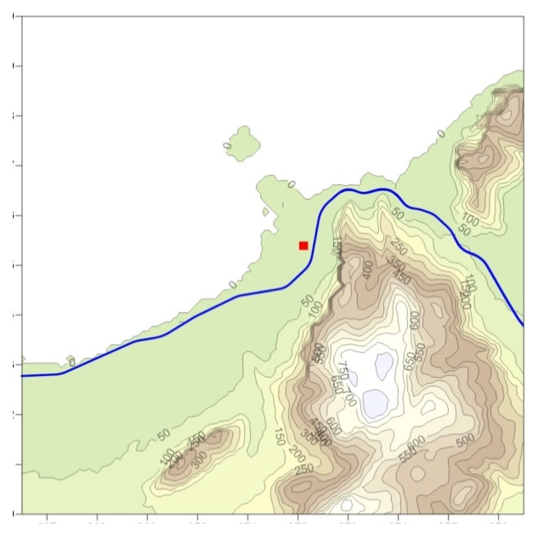
The case study domain of this comparison is crossed by the coastline (Figure 2). Thanks to the availability of a 3D meteorological database specially built for an air quality assessment study of an industrial plant (position indicated by a red square) it was possible to conduct simulations with the two models and compare the dispersion simulation results. Because of the lack of local continuous monitoring and the presence, next to the plant boundary, of a major motorway interfering significantly with the local air quality, it was not possible to effectively compare the results of the two models with measurements.

The study site is complex because of the presence of the coastline and a massif (880 m) that presents a steep cliff (maximum jump of over 400 m) less than 1 km east of the plant, running north-south for at least 4 km and thus being difficult both to overcome and to get around by any plume of smoke. Two other secondary steep orographic structures cannot be neglected in the domain, at about 4 km NE from the plant (520 m) and 5 km SSW (420 m). The domain northwestern portion is instead occupied by the sea.

In a tridimensional dispersion simulation, land use is important, as its inhomogeneity influences the surface layer characteristics and thus roughness and turbulence similarity parameters such as PBL height, $u_{*}$ and L. These last are defined as follows:

$$u_{*}=\frac{ku\left(z_2\right)-u(z_1)}{\ln \left(\frac{z_2-d}{z_1-d}\right)} (“\mathrm{friction} \mathrm{velocity}”)$$

$$L=-\frac{u_{*}^3}{k\frac{g}{T}\frac{Q}{\rho c_p}} (“\mathrm{Monin}–\mathrm{Obokhov} \mathrm{length}”)$$

where:

• k—Von Karman constant;
• u(z_i)—Wind speed at height z_i;
• d—Zero plane displacement;
• g—Gravity acceleration;
• T—Temperature in K;
• Q—Turbulent heat flux;
• ρ—Density;
• c_p—Heat capacity.

These variables are determined in the form of two-dimensional fields and based on the three-dimensional fields of wind and temperature, any other available meteorological variables (e.g., cloudiness or global solar radiation), and the matrices of orography and land-use data, which can describe the horizontal inhomogeneity of the terrain in its response to solar radiative forcing and the resulting inhomogeneity in the turbulence fields that are determined.

Here, land use was extracted from the EEA Corine database [32] and converted into the 14 classes of the CALPUFF scheme (Figure S1 in the Supplementary Material). A total of 46% of cells are over water, 21% over built-up land, 18% over rangeland, 9% over forest land, and 6% over agricultural land.

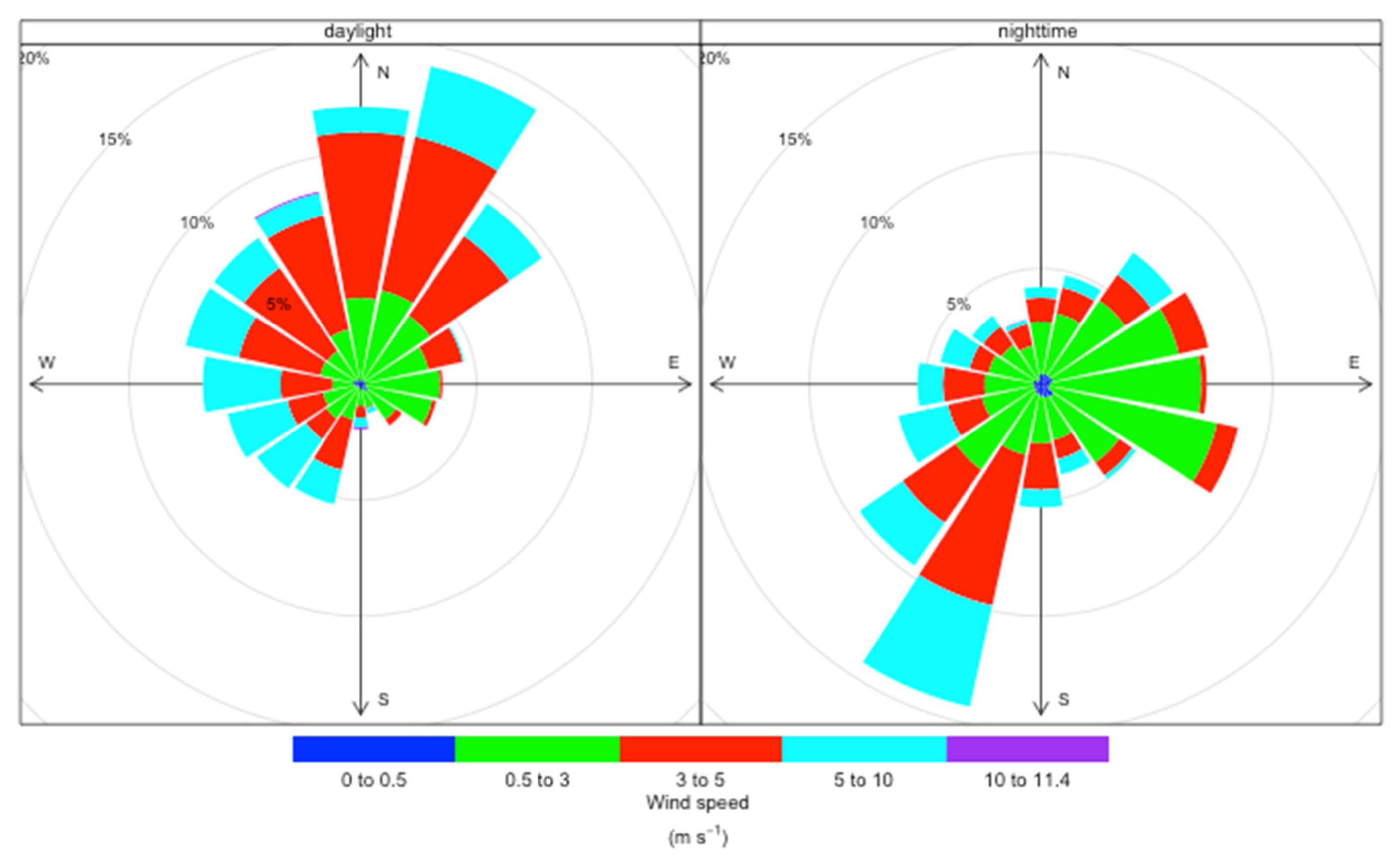
Due to the orientation of the coastline at a larger scale and the presence of the already mentioned cliff, local anemology presents (Figure 3) the highest direction frequencies from NNE during daylight (6 a.m. to 6 p.m.) and SSW during nighttime (6 p.m. to 6 a.m.). During the nighttime, a secondary component of weaker speed is observed from E due probably to both the local orientation of the coastline (land breeze) and the presence of orography (mount breeze).

The computation grid used for the simulations, which coincides with that of three-dimensional meteorological fields, has the following characteristics: 10 × 10 km extension, 101 × 101 cells, 100 × 100 m horizontal resolution. The vertical extent of the simulation domain is 5000 m with the following 15 levels above the reference orography (in meters): 0, 20, 50, 94, 156, 243, 364, 530, 755, 1061, 1471, 2020, 2751, 3720, and 5000.

The simulation lasted a year. Concentrations were calculated on an hourly basis over the entire atmospheric column (up to the domain height) and statistics of the results (yearly averages and maxima) were calculated at the ground level.

Meteorological fields were obtained using a mass-consistent diagnostic model to downscale larger scale 4 km resolution fields (3D wind, temperature and humidity, and 2D precipitation and cloud cover fields) produced by the MINNI national modelling system (“Modello Integrato Nazionale a supporto della Negoziazione internazionale sui temi dell’Inquinamento atmosferico”, [33,34]). MINNI fields are available, at an hourly frequency, for several annual periods, including the one that was used for the study (2007).

For the downscale at the final resolution (100 m), a mass-consistent diagnostic meteorological model was used. To feed the PuM, the meteorological fields were adapted by interpolation, acting in the vertical coordinate from the original “z-top” to the needed “terrain-following” type. The difference between the two types can, in practice, be of some minor significance only far from the ground.

Two real atmospheric pollution sources were considered separately, both situated at a height of about 30 m above sea level. For both, normalized emission rates were considered.

The point source is a stack at a height of about 100 m, a diameter of about 3 m, an exit velocity of about 20 m/s, and a temperature of about 400 K;

The ground-level volume source is a 40 × 10 × 21 m parallelepiped (corresponding to a covered storage area emitting fugitive substances).

Because of their small dimensions with respect to the spatial resolution, the model sources are not actually resolved on the numerical grid. The important difference between the “volumetric” and “point” sources in the present simulations is in the elevation above the ground and physical characteristics, the plume of the “point” source having a higher temperature than the ambient and a positive vertical velocity, thus a vertical rise.

The PuM needed a preliminary sensitivity analysis of some modeling parameters that are not envisaged by the LPM, including the initial σ_x, σ_y, and σ_z coefficients of the volume source (already described) and the terrain adjustment option. For the latter, among the four foreseen, the most advanced one without considering the sub-grid effects, the “plume-path coefficient”, was chosen; the computational resolution (100 m) already being quite high, sub-grid effects can actually be considered negligible.

4. Statistical Indices

A detailed comparison between the results of the two models was developed, based on classical statistical indices. We obtained grids of annual concentration statistics from the simulations to compare with the annual air quality standards (averages and maxima), therefore these agreement indices were applied to the values obtained from the two models at the corresponding nodes of the computational grids.

Three statistical indices were chosen to compare the two simulations in terms of differences between them [12,35]:

Fractional Bias (FB):

$$FB=\frac{\overline{C}-\overline{S}}{0.5 \left(\overline{C}+\overline{S}\right)}$$

where $\overline{C}$ and $\overline{S}$ represent the resulting values of the PuM and the LPM, respectively, averaged over the group of examined domain cells.

It represents the deviation existing between the two models, therefore $FB=0$ (or, at least, close to zero) means that the two models are in great accordance. If negative values are found, the PuM underpredicts the results with respect to the LPM, and vice versa.

FAC1:

$$FAC1=fraction of data that satisfy 0<2\frac{\left|C_{i,j}-S_{i,j}\right|}{C_{i,j}+S_{i,j}}<1$$

where C_i,j and S_i,j represent respectively concentrations calculated by the PuM and the LPM at the domain cell with x index i and y index j.

FAC1 derives from FAC2, a commonly used index of performance of a model in comparison with measurements; the higher the FAC1, the more similar the models are.

Index of Agreement (IA):

$$IA=1-\frac{{\sum }_{i,j}{(C_{i,j}-S_{i,j})}^2}{{\sum }_{i,j}{(\left|C_{i,j}-MM\right|+\left|S_{i,j}-MM\right|)}^2}$$

where MM represents the arithmetic mean of the PuM and LPM concentrations on the entire dataset. As the name suggests, this index reveals the (spatial here) agreement between the two models, therefore the best $IA$ value would be 1; the two models can be considered satisfactorily similar already when $IA\ge 0.5$.

5. Results and Discussion

The maps of calculated annual average and maximum concentrations, for both sources and models, are presented in Figure 4 and Figure 5 and in Figures S2 and S3 (these last belonging to the Supplementary Materials).

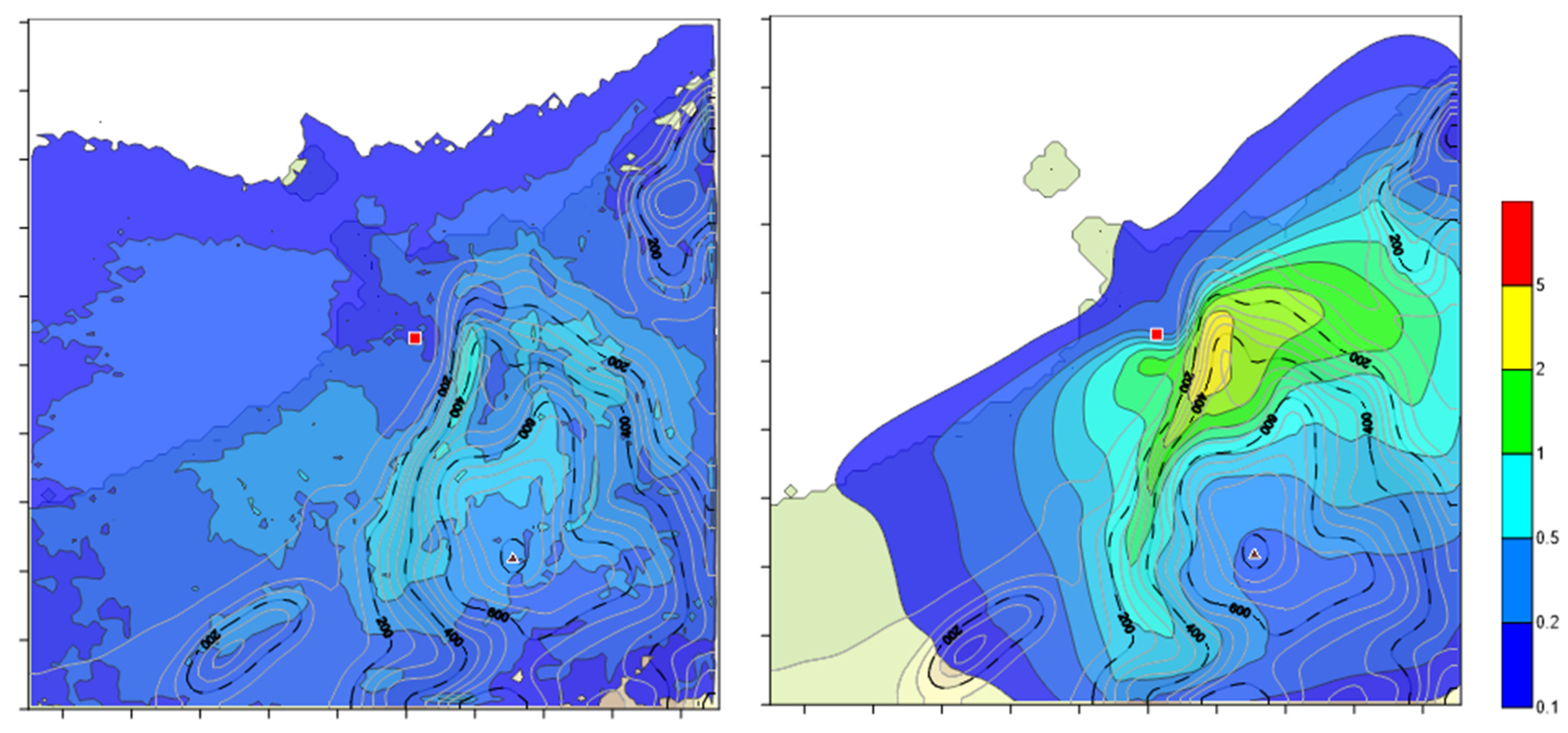
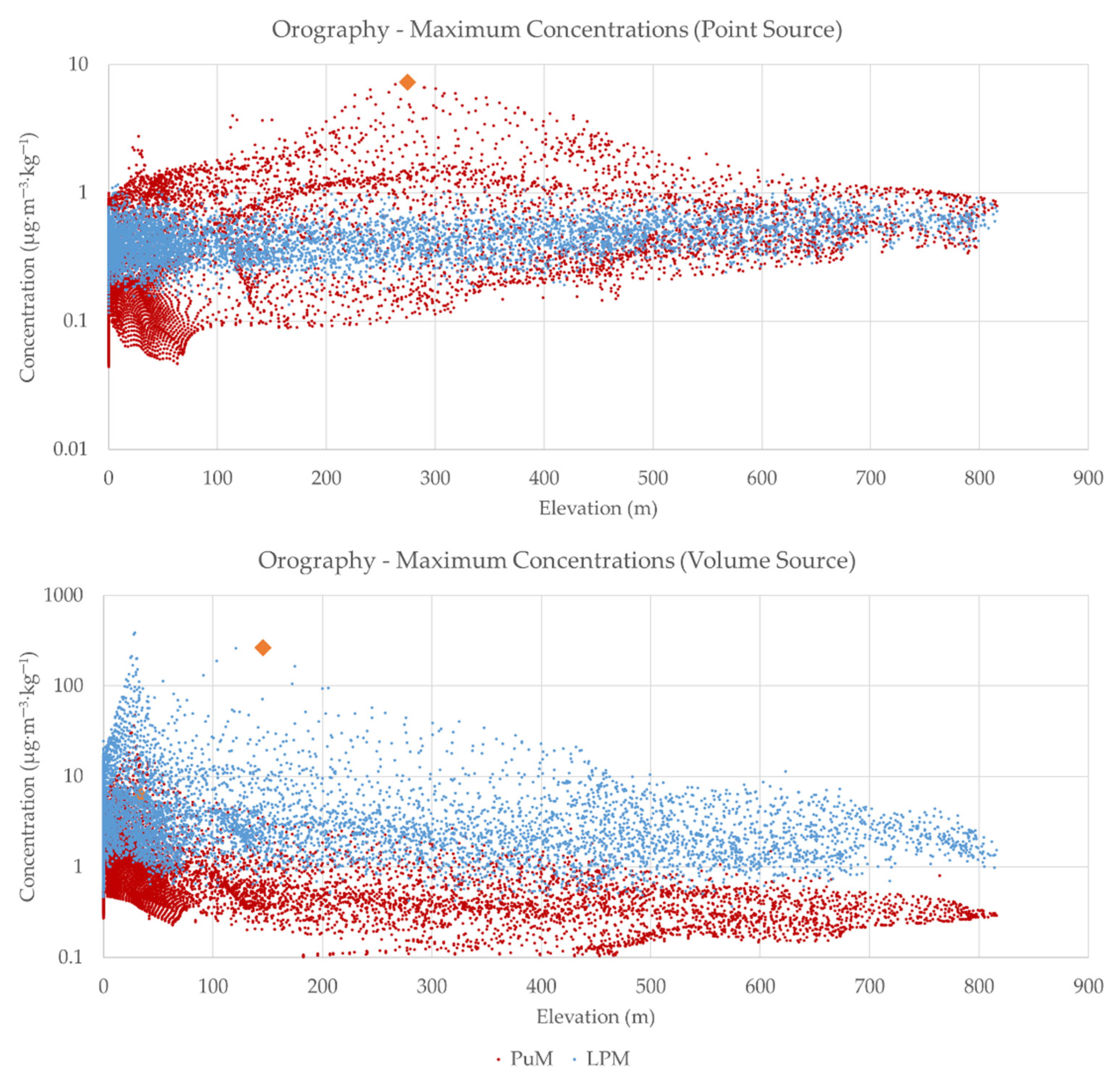
The LPM is, in principle advantaged in reconstructing dispersion in such a situation, because it moves inside the atmospheric flow determined by the complex terrain, thousands of particles following independent trajectories rather than only one; the effect is that it calculates about five times lower concentrations than the PuM on the riff close to the plant when simulating the point source. This does not mean that its concentrations are almost independent of the terrain elevation, as they are still almost ten times higher than those at the same distance on flat terrain (Figure 6). Moreover, any point of its plume being naturally independent of the others, the LPM has a better ability to transport the pollutant from the tall stack in the inhomogeneous atmospheric flow induced by the presence of territorial complexities; for this reason, plume impingements against the complex terrain are not so high as with the PuM (cliffs and other complex geometries are resolved at the same resolution of 100 m of the meteorological fields).

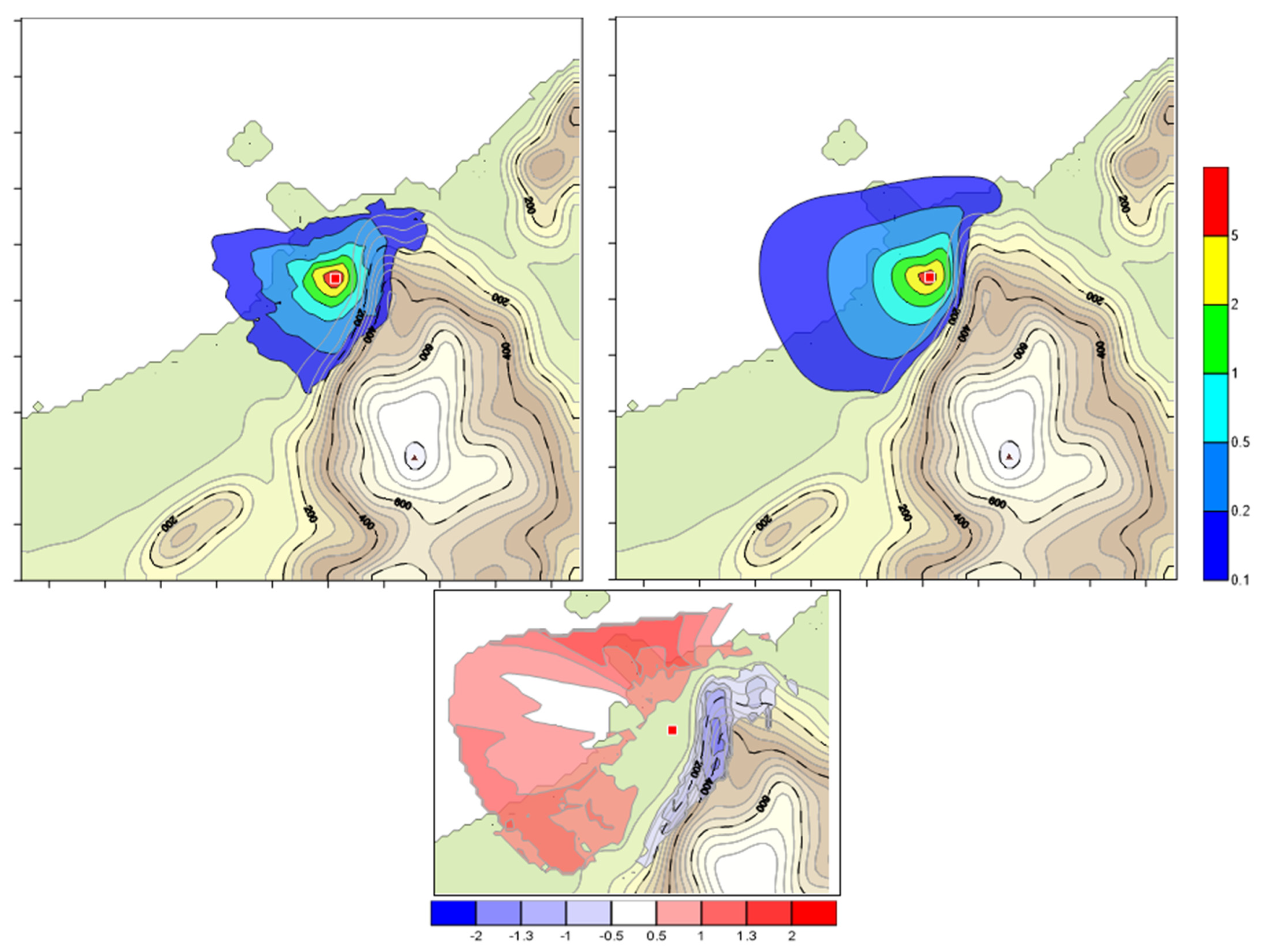
On the contrary, the PuM concentrations are up to six times lower (FB = −1.42) than those of the LPM at that same riff when simulating the volume source (Figure 5, where a zoomed map of FB is also provided for clarity). This can be explained with a null PuM dispersion dependency on the orography of puffs directly emitted at ground level.

Concentrations calculated by the PuM for the point source are not always higher than those by the LPM: on the coastal plain SW of the plant (an urbanized zone), on the slopes of the secondary mount SW from the plant (by which the PuM shows not to be influenced at all), and over water, the PuM calculates about half the concentrations of the LPM. Unlike what is reproduced by the LPM, the PuM does not determine any secondary concentration peak beyond the riff even on the upwind slope of the highest mountain in the domain, which is close to 1000 m and is located southeast of the source at about 5 km.

On average, the two models show similar behavior over flat terrain when the volume source is considered. However, this leads to maximum annual hourly concentrations from the PuM twice as low as those from the LPM.

Figure 6 and Figure S4 (the latter in the Supplementary Materials) show scatter plots of the annual statistics of hourly normalized concentrations versus terrain elevation for the point source and volume source, respectively.

Strong differences are observed between the results of the two simulations across the range of elevations. The main reason for this is related to the different interactions between the plume and the complex terrain simulated by the two models. While in the LPM, all plume particles interact independently with the terrain based on their position, in the PuM only the centers of mass of the puffs interact with the terrain based on position, this leads to distortions of the calculated concentration field at the plume periphery, of which only the largest are adjusted by correction algorithms.

At each elevation, the PuM calculated more scattered concentrations at fixed terrain heights (up to two magnitude orders), than the LPM (still considerable, but limited below one magnitude order) when simulating the point source, while the scatter in the case of volume source is similar between the two models.

On average, if the volumetric source is simulated, the LPM calculates increasingly higher concentrations than the PuM as the altitude increases, up to about three times at 800 m. This is since the PuM plume emitted at ground level from the volumetric source is only marginally affected by orographic effects and can therefore expand freely according to the calculated turbulence intensity at its axis. In contrast, the plume simulated by a more advanced model such as an LPM is more clearly affected by complex terrain effects such as channeling in the valley and confinement due to the presence of steep obstacles.

In the maximum concentrations scatter plots, the bigger orange diamonds indicate the two extreme hourly situations that have been studied and will be described in detail in the following.

Tables S1–S7 of the supplementary material present statistics over the entire domain of annual average and maximum concentrations calculated by the PuM and LPM for the point and volume source.

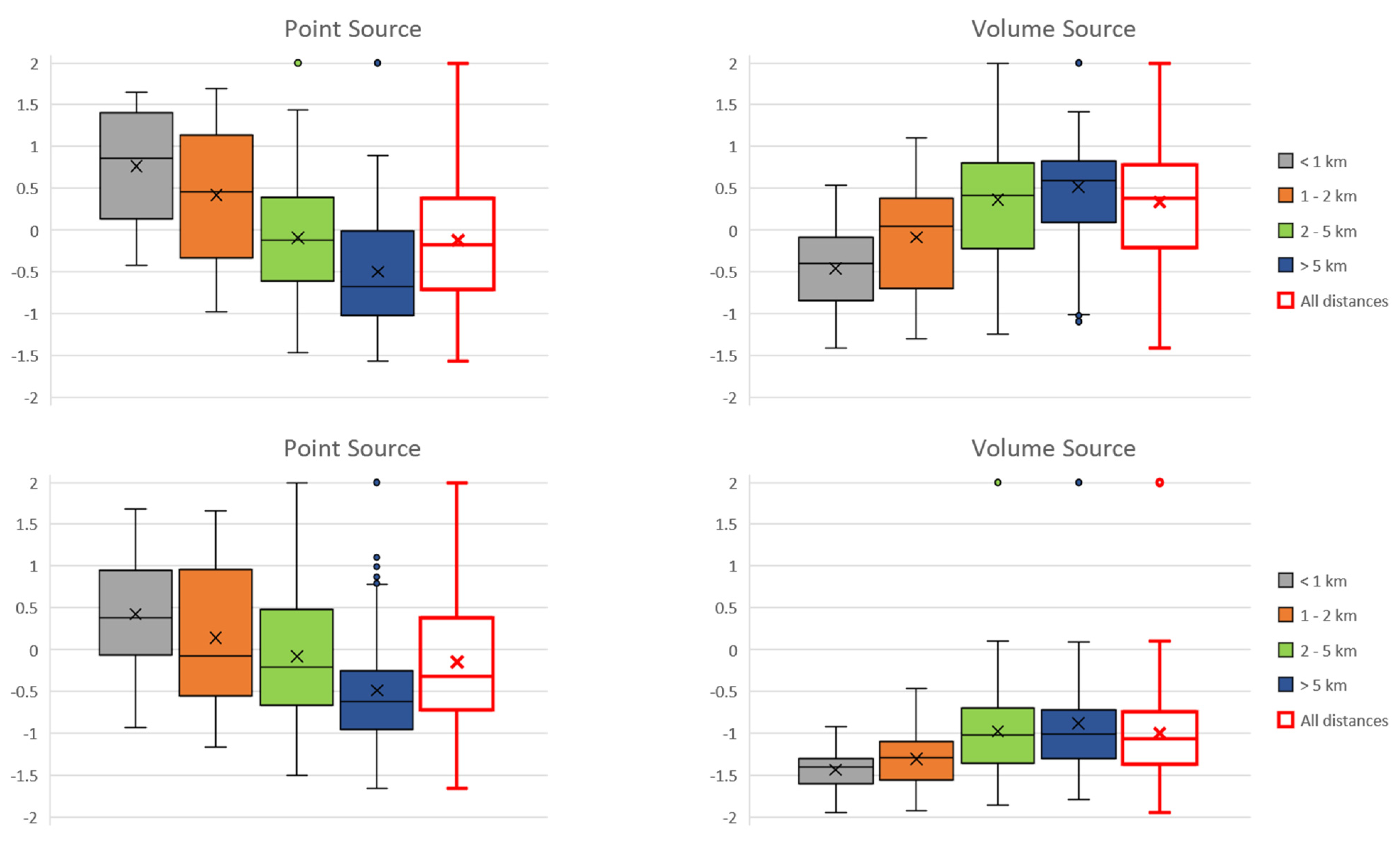
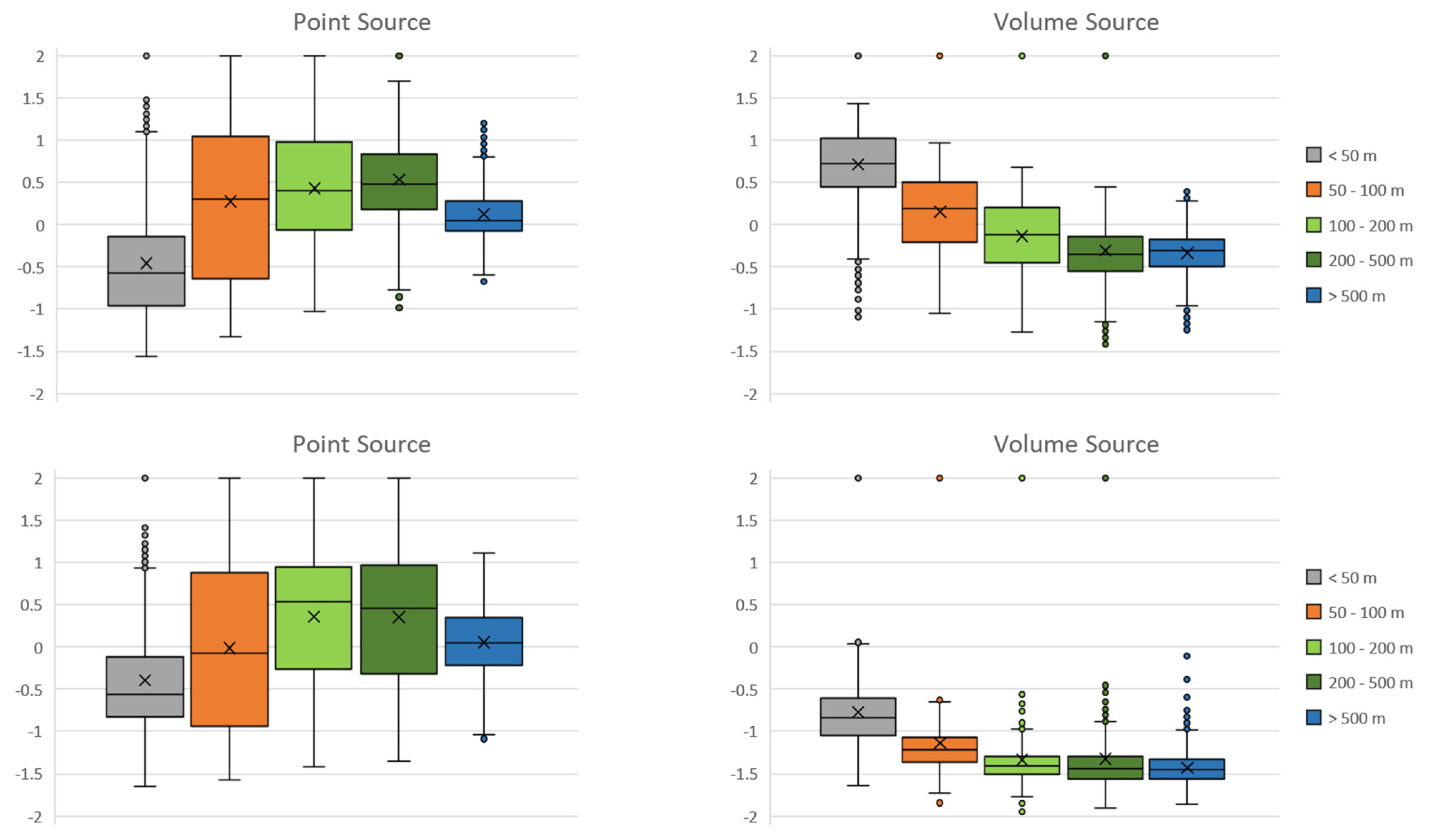
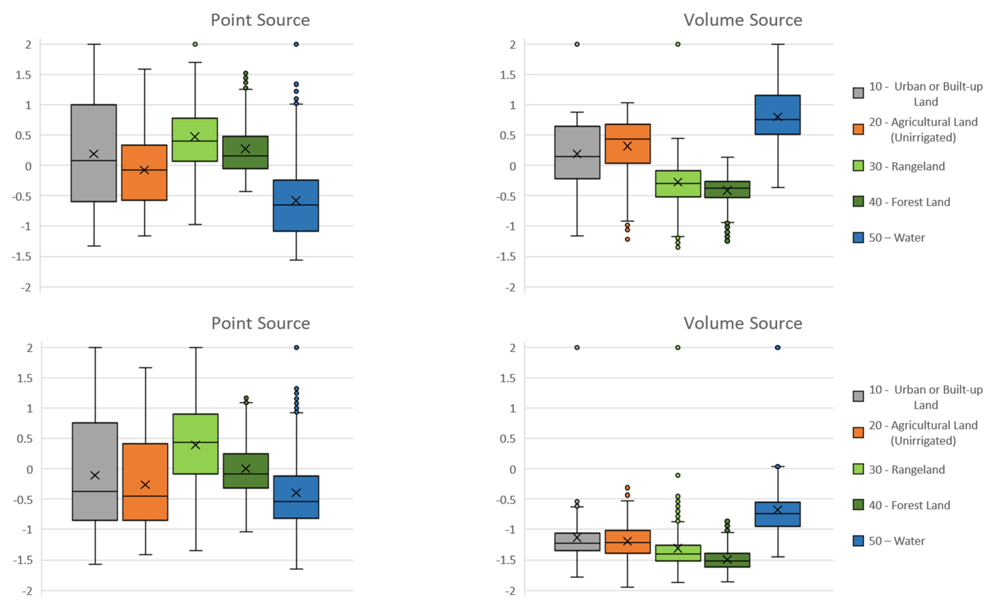
Figure 7, Figure 8 and Figure 9 show the corresponding FB box plots by land use, terrain elevation, and distance from the source. According to the definition above, FB ranges from −2 (zero PuM concentration) to 2 (zero LPM concentration), and is 0 in cases where the LPM and PuM calculated concentrations coincide; if one model calculates a concentration 1.$\overline{6}$ times the other, FB = 0.5 (or −0.5); if that concentration is three times, FB = 1 (or −1).

When considering dispersion from the volume source, the PuM calculates higher statistics of annual mean concentrations than the LPM and much lower statistics of annual maxima (Figure 7). This could lead to an ambiguous assessment of the impact of hypothetical anthropogenic activity, since both long-term and short-term effects are equally important.

The PuM is able to calculate a higher average concentration at distances greater than 2 km, elevations less than 100 m, and over water and agricultural land, consistent with global behavior as the liquid surface occupies nearly 50% of the domain and puffs can disperse to great distances without significant confinement dictated by complex terrain.

Both the annual average and maximum concentration statistics calculated by the PuM are, in the case of the point source, lower than the one by the LPM.

The models are in overall good agreement according to the IA, that is, very close to 1 for the volume source and >0.5 for the point source. This is because more than 65% of the terrain is flat (elevation < 100 m); at higher elevations, stronger differences emerge, as explained in the following sections.

5.1. Volume Source—Annual Statistics

The overall FB boxplot of the annual averages calculated for the volume source (Figure 7, above right, red boxplot) has an interquartile range essentially straddling zero. This confirms that the choice of initial dispersion coefficients made for the PuM is acceptable from the point of view of matching the LPM.

Due to the different ability to interact with the complex terrain when calculating dispersion, which is substantially absent in the PuM, the agreement between the two models is satisfactory only considering annual averages on flat terrain (elevation < 100 m) but degrades rapidly with elevation (Figure 8). As a matter of fact, the change in puff height aboveground is modeled explicitly in CALPUFF if the puff has not already reached the surface [14], thus, in principle, puffs already emitted at ground level are not affected by complex terrain: this appears an oversimplification, at least in presence of particularly steep slopes.

With respect to land use (Figure 9), the agreement between the two models is again ambiguous. For example, on urban land, where the major population lives, it is quite good considering the annual concentration averages (median FB = 0.14) and not so good considering the annual hourly concentration maxima (median FB = −1.22), due probably to the higher dispersive characteristics of the PuM vs. the LPM. Moreover, over water, the FB values are far higher than over the other land types.

5.2. Point Source—Annual Statistics

Considering the dispersion simulations from the point source, an overall agreement between the two models is again satisfactory, even if lower compared to that of the volume source (IA > 0.5 for both annual averages and hourly maxima). Nevertheless, with respect to elevation, the agreement is poor between 100 m and 500 m, in particular at the first cliff closer to the source (median FB = about 0.5). Therefore, due to its characteristics of less dispersion and particle independence from its own axis, the LPM plume shows its higher ability to overcome or circumvent even very steep obstacles without the strong collision simulated by the PuM.

Other interesting differences in the interaction with the complex terrain and the 3D wind field will be shown in the next sections.

5.3. Selected Peak Hourly Situations

For a more complete comparison between the two models, two peak hourly situations were selected inside the examined annual period. They correspond to the shown orange diamonds in Figure 6.

The first selected situation corresponds to the highest hourly maximum concentration at elevation >100 m, calculated (by the LPM in this case) when simulating the volume source, and is encountered at 7 a.m. on 29 March at an elevation of 100–200 m with an estimated normalized value of 264.3 µg h m⁻³ kg⁻¹.

The second relates to the absolute maximum hourly concentration calculated (by the PuM) when simulating the point source and is encountered at 8 p.m. on 26 June at an elevation between 200 and 300 m and assumes a normalized value of 7.3 µg h m⁻³ kg⁻¹.

5.3.1. Volume Source—29 March 2007, 7 a.m.

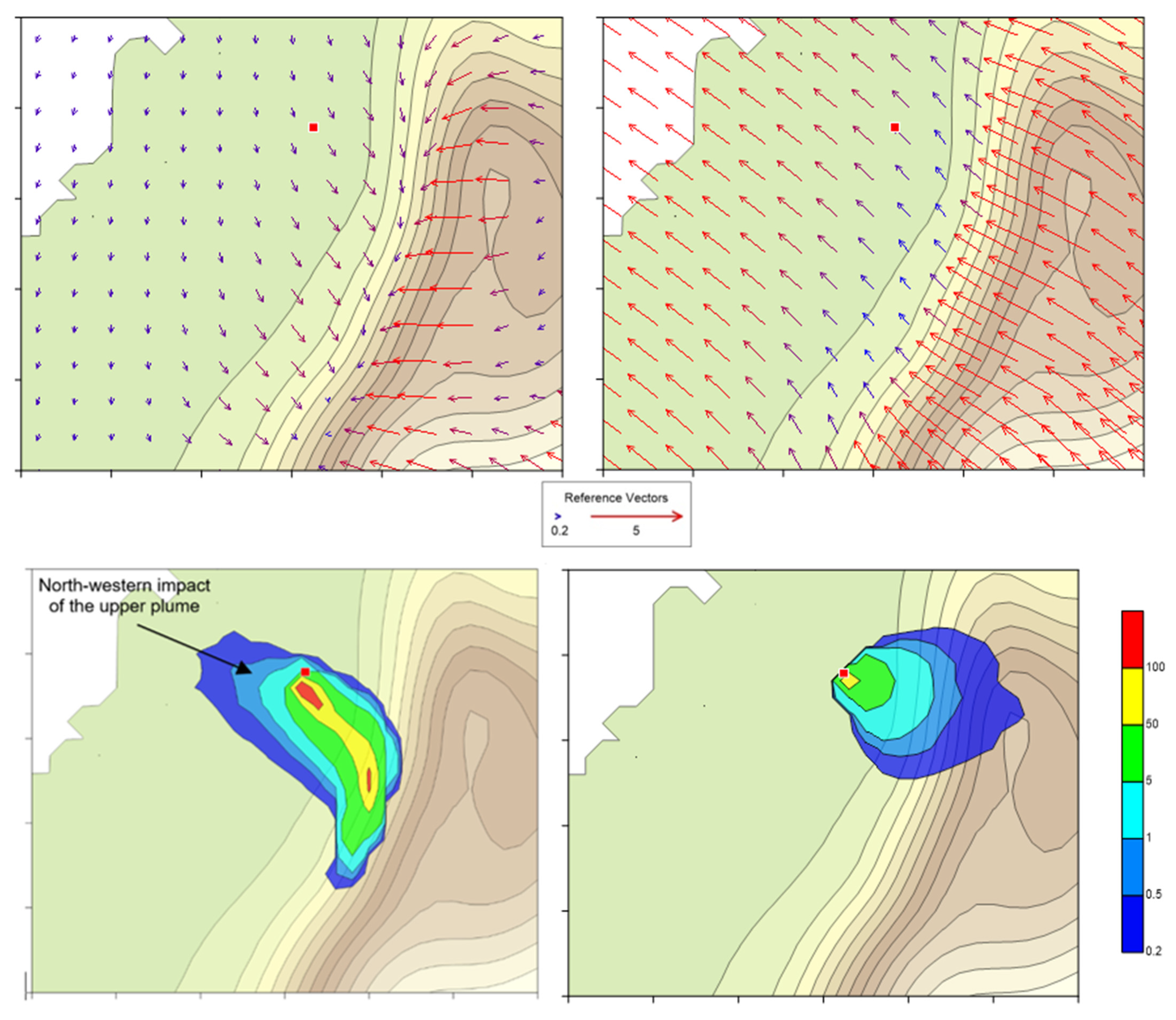
Figure 10 presents the wind field at two levels and the ground level hourly concentration calculated by the two models on 29 March 2007 at 7 a.m. (dawn time: 6:55 a.m.) when simulating the volume source.

Being in a transition phase from nocturnal to diurnal conditions, a thick layer of weak northern wind on the plain where the source is located is overlaid by an upper layer with a moderate south-eastern wind. In this situation, we would expect that a ground-emitted plume is trapped and confined close to the steep upward slope, as simulated by the LPM. The PuM, on the contrary, does not show relevant plume interactions with the terrain even in such a complex situation: the plume slides up the steep slope without any relevant confinement.

Moreover, the plume portions that reach the upper layers are expected to be transported back towards the NW. Effectively, the LPM simulation shows a relevant impact towards NW, upwind of the source; this effect is not simulated by the PuM, as the entire plume is coherent with its axis and is transported SE according to the ground level wind.

5.3.2. Point Source—26 June 2007, 9 p.m.

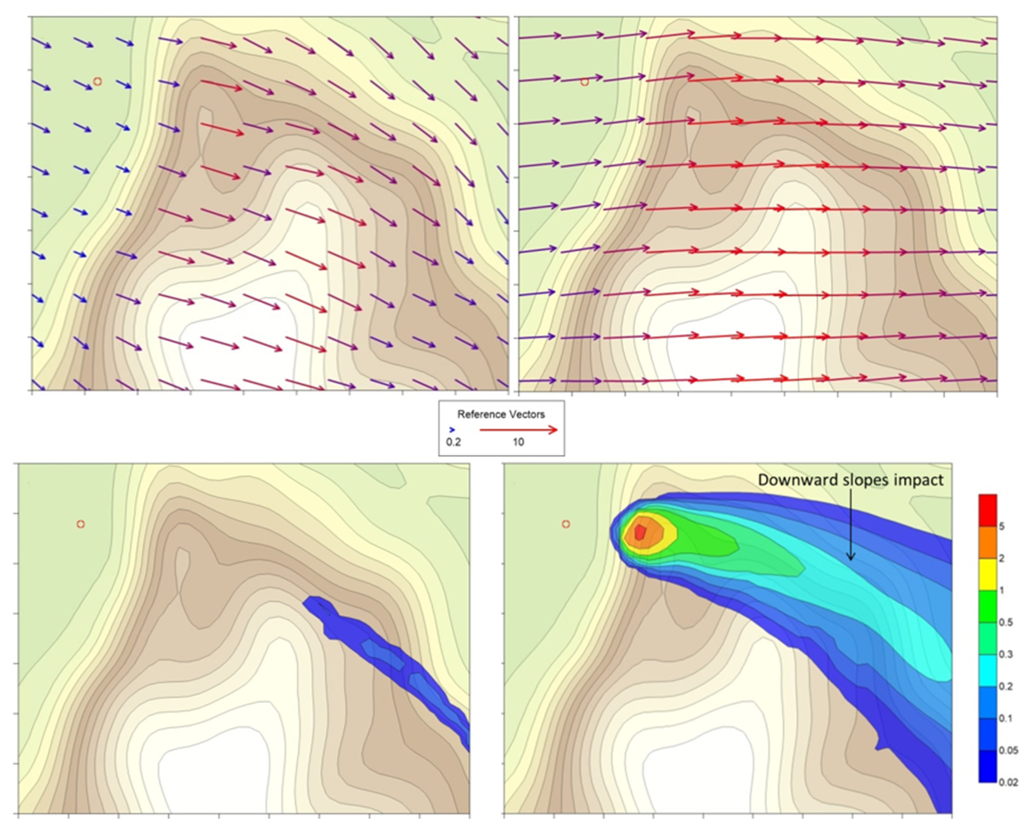
Figure 11 (zoomed maps to better observe the details) presents, respectively, the wind field at two levels and the ground level hourly concentration calculated by the two models on 26 June 2007 at 9 p.m. (sunset time: 8:35 p.m.) when simulating the point source. The wind is moderate at 500 m over flat terrain and weaker at 100 m. At a higher elevation, it blows from WSW with a slight clockwise rotation from W to E. At the lower level, the wind rotates, with respect to the upper level of 30° to 45°, and tends to circumvent the main mount from N. Above the coastal plain, the 100 m wind heads directly toward the slope of the mount.

In such a situation, we can expect that a tall plume such as the one emitted by the examined stack in unstable or neutral conditions (or at least its upper part) passes north past the main first steep climb without interacting with it so much, the lower part possibly feeling an extra horizontal dispersion due to the strong wind rotation between 500 m and 100 m. Assuming the plume rise similar in the two models, while the LPM shows the expected behavior, thanks again to the possibility of following thousands of independent trajectories in the 3D flow, the single trajectory representing the PuM plume axis appears trapped in the lower layers, thus going too early to level off the complex terrain.

Another notable difference between the two models is the impact on downward slopes, which, according to the PuM, is far more important, as the plume, even at distance from the source and so already widely dispersed, is considered coherent with its axis elevation over the ground, thus not feeling the terrain moving away at its borders (the opposite effect over upward slopes is somehow adjusted by CALPUFF introducing the so-called “flagpole receptors” [14]).

6. Conclusions

With the objective of studying the behavior of a PuM in reproducing maps of environmental concentration statistics for evaluation purposes (annual averages and maxima) in a one-year simulation, it was compared with an LPM, a model with, at least in principle, more advanced capabilities to reproduce 3D dispersion phenomena in complex terrain.

This approach may be useful to show the limitations and advantages of using models if it is required to analyze a complex situation in the absence of—or in the impossibility of—using experimental air quality measurements.

The same 3D hourly meteorological fields were used for both models. Several statistical comparison tests were conducted, considering separately a point source and a volumetric source with the realistic physical characteristics and normalized emissions of a nonreactive pollutant.

Intercomparison was performed through the analysis of 2D maps of ground-level concentrations, scatterplots, and three classical indices calculated on the individual values of the maps of annual concentration statistics. To correlate the differences between models with site characteristics, these concentration statistics were analyzed not only globally, but also according to distance from the source, elevation, and land use classification.

Any quantitative results in terms of differences between the two models were shown to be robust to the uncertainty caused by the dependence of the LPM on the number of particles emitted and the cell size of the concentration domain.

The analysis shows that the plume dispersion around its axis is lower in the LPM than in the PuM across all land use types except water surfaces.

If a high, hot point source is considered, this leads the PuM to calculate higher ground-level concentrations than the LPM on flat land within a 2 km radius and lower concentrations on water.

A less-dispersed plume in the LPM generally does not necessarily lead to higher ground-level concentrations when encountering complex terrain because of the ability to interact with the 3D wind field at any point in the plume rather than only in its axis, as in the PuM. This leads the LPM to less uncertainty in assessing impacts at terrain locations with the same characteristics (height or distance from the source).

Greater differences are observed when plumes interact with complex terrain, with the LPM showing virtually better capabilities in reproducing effects such as plume upsloping and downsloping, deflection, channeling, separation, and confinement.

In contrast, the behavior of the PuM in complex terrain is observed to be at least unclear. If a high, hot point source is simulated, it is shown to exaggerate the impact on the first significant obstacle encountered and to neglect the presence of subsequent, equally important ones.

In the case of a cold volume source at ground level, the PuM exhibits virtually no interaction with the complex terrain and higher calculated concentrations at long distances since the ground-level puffs can be freely dispersed without any containment by orographic obstacles.

In addition, the PuM shows greater uncertainties in the parameterization of the initial source volume dispersion, which could greatly affect the calculation and thus the assessment results.

The analysis suggests that the suitability of a PuM should be carefully considered when computing the dispersion of air pollutants over particularly complex terrain, as it can lead to very different results than a more advanced dispersion tool.

Our advice is to always prefer more advanced dispersion models when studying both the short- and long-term atmospheric impacts of fugitive air pollutant emissions at ground level and, in complex terrain, at least at distances of more than a few kilometers, in the presence of hot and high point sources.