1. Introduction
Spatial continuous data, or spatial continuous surfaces, play a significant role in planning, risk assessment and decision making in environmental management [
1]. Sparse networks for measurements therefore have to be carefully considered as representative of non-measured spaces. Interpolations are key solutions for estimating unknown continuous values, while geostatistics represents the most accurate technique of that methodology [
2]. Moreover, analyzing the spatial distribution of air pollutants in populated areas is essential for urban management and territorial planning.
Geostatistical interpolation methods have widespread use in estimating individual exposure to outdoor air pollutants, and in modeling atmospheric phenomena, among other uses [
3,
4,
5,
6]. The toxic nature of particulate matter (PM
2.5 and PM
10) to human health has promoted the extensive use of geostatistical methods with geographic information system (GIS) tools to analyze the spatial distribution of these pollutants. Although some of the air quality interpolation approaches have been carried out by deterministic methods with excellent results [
7,
8], other studies have reduced errors using geostatistical methods that employ inverse distance weighting [
9], ordinary kriging [
10,
11] or empirical Bayesian kriging [
2,
12]. Spatiotemporal variabilities have also shown to be a great fit, with geostatistical methods of interpolation for PM
2.5 and PM
10 having been used, for instance, in Cusco, Perú [
13]. In addition, [
14] found geostatistical techniques to be the best fitting interpolation model for 71 interpolations of air pollutants.
In a similar way to air pollution analysis, various studies have carried out different kinds of spatial interpolations of atmospheric variables, such as temperature, pressure, relative humidity (RH) and precipitation [
15,
16,
17,
18]. The necessity of analyzing the influence of weather variables on air quality is justified by recent findings on the topic, where PM
2.5 has been strongly related to meteorological parameters [
19,
20]. Zhao et al. [
21] found that relative humidity, precipitation and pressure had more influence on PM
2.5 than temperature or wind speed. However, the influences of meteorological variables are also related to location. Although variables such as precipitation and temperature have been found to have positive and negative influences, respectively, on PM
2.5 in countries such as Japan [
22], precipitation has been found to have an inverse relation in the USA [
23]. New machine learning methods [
24,
25] have been also widely used to study the relationship between air quality and meteorological variables.
In the present work, in order to determine which of the meteorological variables is the main contributor to changes in PM
2.5 in Cartagena de Indias (Colombia), spatial analysis was conducted. The aim of this paper is to introduce the relation between PM
2.5 and available weather records. In the study, continuous spatial representations and estimates of PM
2.5 concentration data, temperature and relative humidity in Cartagena were studied by the IDW and ordinary Kriging methods, which considered virtual information points. In addition, the spatial average data of fine particle variables, temperature and relative humidity were estimated across the city by considering the influence of wind speed on PM
2.5 concentrations. Fine particles such as PM are harmful for human health as they corrode the alveolar wall in the lungs after being breathed in [
26]. Among all PM particles, PM
2.5 is the most harmful for human health [
27].
Location
This study focused on Cartagena de Indias, in Colombia (10°25′30″ N, 75°32′25″ W). Cartagena is one of the most important urban areas in the Colombian Caribbean region.
Basic regulations on air quality are derived from the Environmental Ministry of Colombia (Ministerio de Medio Ambiente y Desarrollo Sostenible), who decreed that by 2011, every main urban area must have a network for measuring air quality. The Environmental Public Agency of Cartagena (EPA-Cartagena), uses an algorithm to calculate the air quality index in which PM
2.5 values between 15 and 40 µg/m
3 (over 24 h) are considered to be a moderate influence on human health, and values between 40 to 65 µg/m
3 are considered harmful for human health [
28].
In Cartagena de Indias, the scarcity of technical resources has not allowed for the development of an extensive network (in a spatial and temporal sense) of measuring stations for the continuous observation of pollutants and weather variables. This situation is a very common one in developing countries around the world [
29,
30,
31,
32,
33].
Previous measurements of air quality in Cartagena [
34] have demonstrated that the concentrations of gases, such as SO
2 and CO
2, were below the limits recommended by national regulations. The mean values of PM
2.5 in Cartagena have been found to be 25.5 µg/m
3, rendering the city with the second highest mean PM values, surpassed only by Medellin at 30 µg/m
3, but which has double the population of Cartagena.
Cartagena de Indias’s climate corresponds to an equatorial/subtropical type. With a mean temperature of 28 °C and a mean relative humidity of 77%, Cartagena is usually expected to have a rainy season (August to November) controlled mainly by the displacement of the ITCZ (Intertropical Convergence Zone) to northern positions at 8° latitude [
35,
36]. The southward displacement of the ITCZ brings a displacement of the Azores High and a dry season with strong northeastern winds [
37].
2. Methodology
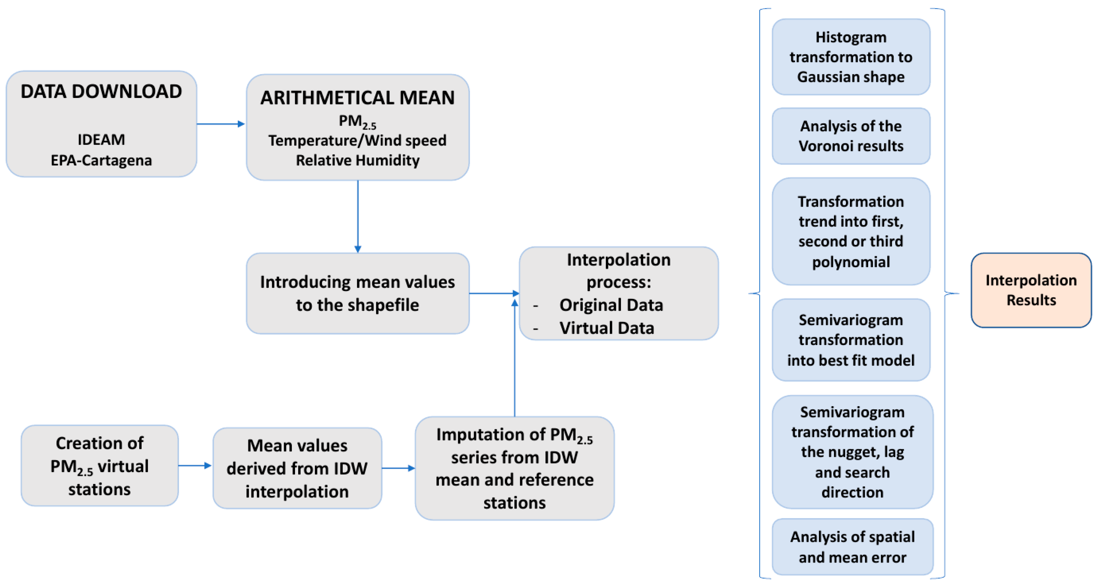
Different spatial analyses were carried out to determine the spatial distribution of fine particles and meteorological variables. The main objective of the spatial interpolation was to predict the PM
2.5 concentrations at ground level and the meteorological variables of Cartagena. The workflow is presented in
Figure 1.
2.1. Data Source
Data records of PM2.5 and weather variables were obtained from different public agencies and some non-governmental organizations.
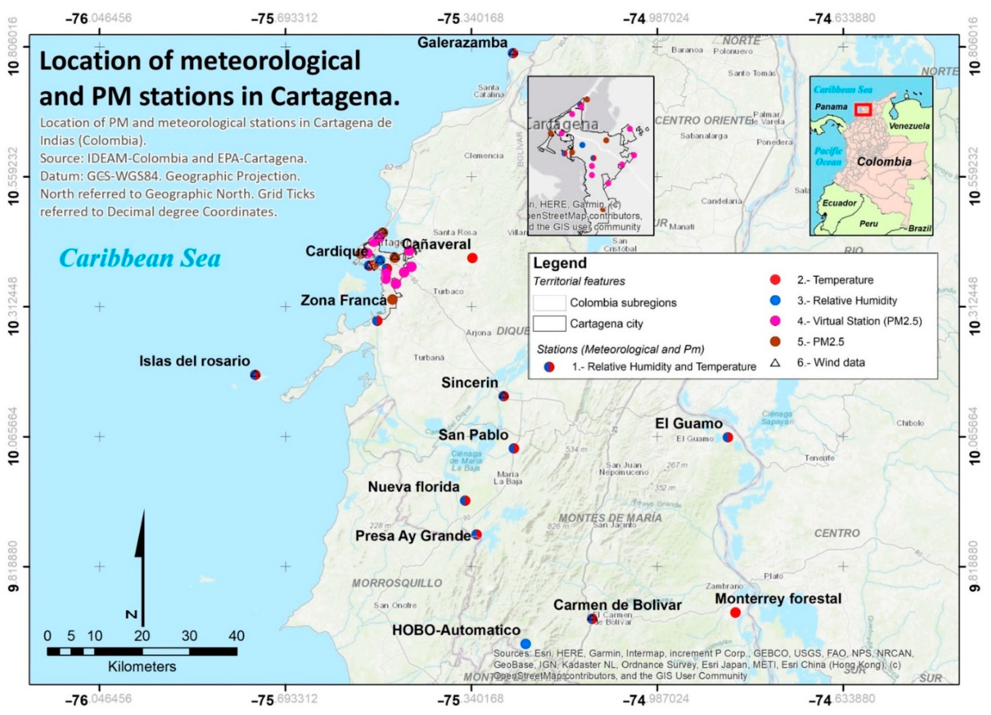
A total of 21 weather stations were selected, with the data analysis focusing on the temperature, wind speed and RH (
Figure 2). The location and source of the information for each meteorological station, and the variables collected, are shown in
Table 1. Most of the stations presented data for the years 1971 to 2001, whereas 5 stations (the main ones within the Cartagena urban area) had data from 2014 to 2015, and the rest recorded data from 2019 to 2021. The relatively stable climate of this region of Colombia allowed for the study to be carried out with homogeneous data.
The series of data analyzed for relative humidity were expressed at an hourly time scale, whereas temperature series were expressed at hourly and daily time scales. Both variables were derived from measurements made by the meteorological agency of Colombia, IDEAM (for its initials in Spanish), the Environmental Public Agency of Cartagena network (EPA-Cartagena, for its initials in Spanish), the oceanographic center CIOH (for its initials in Spanish) and the non-governmental organization, Oasis Jacquin. The PM2.5 and PM10 data series available were monthly and were derived from daily measurements carried out by the EPA-Cartagena public agency. The analyzed temperature data series were of an hourly and daily nature and were derived from measurements carried out by all the aforementioned organizations.
Wind speed data were downloaded from the IDEAM-Colombia network of stations and from the EPA-Cartagena air quality measurements stations, which had anemometers for measuring wind. The data downloaded had 10-year records (2011–2021) in the case of the IDEAM stations [
38] and 2-year records (2014–2015) for the EPA-Cartagena stations [
28,
39]. In total, up to 10 stations with wind data were analyzed.
Meteorological data corresponded to different time periods ranging from 1971 to 2021. Records of pollutant concentrations of PM
2.5 (µg/m
3) and PM
10 (µg/m
3) were collected by the EPA-Cartagena [
39,
40,
41] environmental public authority between January 2014 and September 2017 (
Figure 2 and
Table 2). Data concentrations of PM
10 were transformed to PM
2.5 data assuming a PM
2.5/PM
10 ratio of 0.5 units [
42,
43,
44]. La Bocana Station, which measures PM
10, was useful because it had estimations from the northwestern side of the city, also offering more stability for the interpolation process through the addition of more data.
For some of the interpolation analyses, a 30 m. resolution digital elevation model was used, provided by the Aster program [
45].
2.2. Pre-Treatment of Data Series
Using the Rstudio software [
46], hourly data of temperature and relative humidity were transformed into maximum and minimum daily values in order to homogenize all the variables to a daily time scale.
Then, daily values of different basic statistics were calculated for the whole series, such as the arithmetic mean, the median and the standard deviation. The arithmetic mean was the main parameter that fed the subsequent interpolation analyses. These parameters were calculated for all the variables of this study.
In the case of wind parameters, graphs of the “wind compass” type were derived, which indicated the average speed and direction. The wind direction showed significant inconsistencies between stations, so this parameter was omitted from the analyses. Omitting wind direction implies a lower accuracy in the results of PM
2.5 estimated values. The wind direction exerts a great influence on the redistribution of pollutants over certain areas, creating spatial differences [
47,
48,
49].
2.3. Spatial Data Analysis
To have a good understanding of the internal structure of the data, ArcGIS was used, which offers a set of tools through which the distribution can be explored in order to identify global trends and to calculate the spatial autocorrelation of data series [
50,
51].
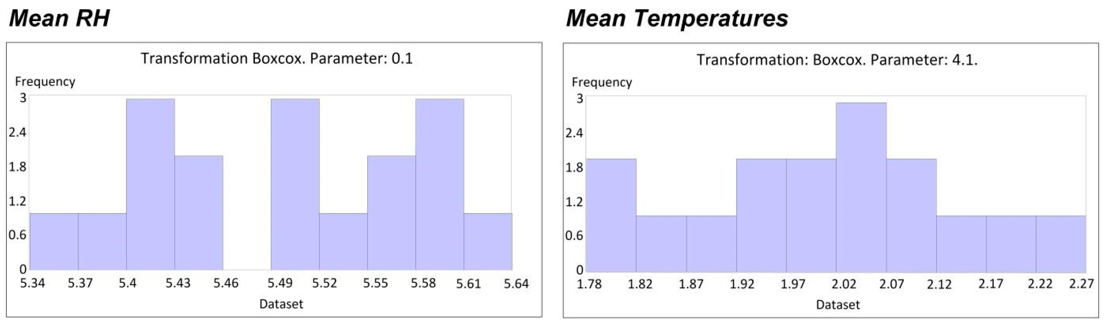
The tool used to test the normality of the data series was the histogram. Histograms were transformed using logarithmic functions and Box–Cox functions, until the best fit to a Gaussian shape was achieved. When the spatial representation of the data presented a Gaussian shape, a more transitional interpolation without any “breaks” or discontinuities in the data was achieved using a continuous (or smooth) search neighborhood. Box–Cox transformations were selected according to a numeric vector of finite values indicating which powers should be used for the transformation. Those values were expressed as subscripts.
Additionally, the spatial trends of the data series on an X-Y-Z graph were also analyzed for each variable. The Z-axis was represented vertically, in order to give a 3D position according to the values of each of the stations (represented by points). The greater the value was, the “higher” the position given in the Z value. The X and Y values corresponded to the geographic coordinates of each of the points representing the stations. In this case, on the graph, it may be seen that the polynomial trend was the one that best fit the trend of the data according to the two cardinal axes (North–South and East–West) represented by two perpendicular planes.
Subsequently, the semivariograms of the data for each variable were analyzed. A semivariogram is the graphical representation of the distances and values for each variable, and they provide a representation of the autocorrelation. They measure the degree of dissimilarity [
52] and represent the relationship between the distance of two points (stations in the case of this study) and their differences in value. The lower the difference and the distance between two points, the closer the semivariogram to the axis origin in the graph. Semivariograms are composed of a series of parts including the nugget and the lag size. The nugget is the separation distance of the semivariogram values with the “Y” axis. If the interception of the values of the semivariogram is within the value 2, then the nugget is 2. The value should be greater than 0. The lag size is the size of a distance class into which pairs of locations are grouped to reduce the large number of possible combinations.
Equation (1) shows the mathematical representation of a semivariogram, where yh is the representation of dissimilarity, z (xi) and z (xj + h) are pairs of samples (the stations in this case) in classes within a given distance and direction, and N(h) represents the number of data pairs in each of the classes.
Autocorrelation is maximized when performing an interpolation through geostatistical methods. Geostatistical processes are based on the autocorrelation concept, so the distance and direction between points of values govern the estimated values. Predicted values of the unknown attributes have less error when the spatial autocorrelation approaches the maximum [
5]. In this study, in order to achieve autocorrelation, the data were adjusted from a predefined theoretical model to the experimental semivariogram. Adjusting the semivariogram was carried out by adjusting a theoretical model to the measured values until a best fit was achieved.
The interpolation of mean relative humidity during the dry season was ruled out because the data could not be adjusted during the process, due to the lack of homogeneous records. Even so, the process was attempted, but a great spatial error was generated (>12%), and the error range for other processes was between 0.31% and 2.87%, so the analysis was rejected. The geostatistical analyst tool estimated two statistical error calculations for each interpolation: an estimated error for each location on the data source station and a spatial error for each area of the interpolation.
2.4. Interpolation Analyses
Interpolations under different situations have been used to provide spatially continuous estimates of fine particle and weather records [
53,
54,
55,
56]. In this study, geostatistical techniques were used to estimate the behavior of variables affecting human health in Cartagena with minimal error. By adjusting these data through pre-processing, it is possible to generate a result with reduced error [
2,
57,
58].
The pieces of software used for data interpolation were ArcGIS 10.5 and ArcGISs Pro 2.6.0 [
59,
60]. ArcGIS 10.5 Geostatistical Wizard tool enabled data exploration prior to interpolation generation, which allowed for further tuning of internal data in ArcGIS-Pro. Interpolations were performed for all available variables, generating 9 interpolations, whose specifications are listed in
Table 3.
The variables subjected to interpolation were as follows: average temperature, mean temperature during the dry season (December to April), average temperature during the wet season (August to November), mean RH, average RH in the dry season, average RH in the wet season, mean of PM2.5 and PM2.5 in the dry season, mean of PM2.5 in the wet season and mean wind speed.
All the results were adjusted to obtain a 30 m spatial resolution raster.
Since in some cases PM
2.5 records for interpolations were scarce, a series of virtual stations were created at random and peripheral locations, which supported the interpolation process. The creation of virtual stations is a methodology widely used in air pollution studies [
61,
62] and in interpolation of climatological variables [
63,
64,
65]. Data from these stations were mapped considering an estimate according to the inverse distance weighted (IDW) method, which interpolates PM
2.5 concentrations.
In the IDW interpolation analysis, the mean spatial values at selected locations were derived to feed those virtual stations, with new values obtained for the corresponding area of each new station. Those mean values were used for an imputation process (gap-filling) where the estimated value through the IDW technique is the reference mean value. The imputation process was carried out according to Paulhus and Köhler’s [
66,
67,
68,
69,
70,
71,
72,
73,
74,
75,
76,
77,
78,
79,
80,
81,
82,
83] methodology in order to obtain PM
2.5 values at stations for each month. The new monthly data of each virtual station were related to reference stations (the closest existing one with complete data), so it could take the monthly variability from existing data. The mean of that monthly PM
2.5 interpolated value fed the data for the virtual station in the interpolation. Equation (2) expresses the procedure:
Coefficients “
a” and “
b” were obtained according to Equations (3) and (4):
where
is the mean of the reference station,
is the mean of the incomplete station,
represents the covariance of both stations and
is the variance of the reference station. The reference value is the PM
2.5 monthly value of the selected station with completed data.
Therefore, the value used in the virtual station was the one derived from the IDW interpolation and later imputed monthly in order to obtain different season values and a general value for the whole period (2014–2017). Introducing virtual stations can lead to a spatial representation with more transitional values that is close to the average, as this methodology is not sampling real variability.
The use of the original data in the PM2.5 interpolation process (5 stations) would have led to a failure of the operation, since they contained fewer stations than those required by the software tool. Therefore, virtual stations were needed for the tool to work in a place such as Cartagena, where scarcity of data is a problem. The implications of an interpolation process within the limit of stations (8–10 stations, depending on the spatial distribution) would lead to less semivariogram model adjustment and a loss of accuracy. In the case of this study, the minimum number of stations used for interpolations was 10. This number of stations is enough for the tool to work but requires a longer processing time due to the need of adjusting the semivariogram to the model used. The problems with adjusting the semivariogram do not necessarily imply a loss in accuracy but lead to a longer processing time for adjusting other associated parameters such as the lag size or nugget.
The interpolation results were divided into predictive maps and spatial standard error maps. The error maps were used to calibrate the quality of the data in each area of Cartagena, and to propose the installation of new monitors or meteorological stations in the areas with the greatest spatial error.
Although a calibration process was not possible, the interpolation returned results of the error and standard error between the measured values in each station and the corresponding pixel predicted value in the raster. These errors were relatively low, with a maximum of 1.23 and 1.53 obtained for the error and standard error, respectively.
Interpolation techniques such as inverse distance weighting (IDW) base their operation on gradual changes from the inverse distance, according to Tobler’s [
84] first law [
68,
69]. Conversely, geostatistics techniques consider relative distance, according to the internal structure of the data, based on Tobler’s second law [
70,
71]. Thus, in conventional methods such as IDW, information on spatial correlation is not used, whereas geostatistical estimation considers both spatial and distance correlation [
72].
2.4.1. Inverse Distance Weighting (IDW)
One of the most commonly used deterministic methods is IDW [
73]. The IDW algorithm is based on the notion that the degree of influence of nearby monitors should be greater than the dependence on distant monitors. Basically, in this case, the unknown values can be calculated as a distance-weighted average of the sample point values. The weights (
λi) are calculated as follows (Equation (5)):
where
λi is the weight of the monitor
i,
Di is the distance between station
i and an unknown point, and
α is the weighting power.
IDW analysis was performed to obtain the mean values for the data series ascribed in the virtual stations of PM2.5.
2.4.2. Ordinary Kriging (OK)
Similar to IDW, the OK method calculates a weighted average of concentrations at measuring stations. However, through this algorithm, the weights use a distance function based on a variogram [
4]. The OK geostatistical function assumes the model described below (Equation (6)):
where
X0 is the unknown attribute,
n is the neighboring values of the samples and
information points are linearly combined with weighting
.
The existing literature recommends the use of simple kriging for interpolations that observe defined spatial trends [
74,
75]. However, although spatial trends were observed in the data in this study, the use of this methodology was rejected because it did not have fully reliable series, so the OK feature was used. Ordinary kriging was used for analyzing the variables of mean temperature, mean temperature during the dry season, mean temperature during the humid season, mean relative humidity, mean relative humidity during the dry season and relative humidity during the humid season.
2.4.3. Empirical Bayesian Kriging Regression Prediction (EBK-RP)
The interpolations of wind speed and PM distribution were derived with the empirical Bayesian kriging regression prediction tool, present in ArcGIS Pro applications [
2,
76,
77,
78,
79]. Given that wind speed may have a strong dependence on the topography [
80,
81], and PM could be related to the weather variables studied in this research, the empirical Bayesian kriging regression prediction tool was used. This tool allows for the introduction of explanatory variables having a known influence on the main variable in raster format. The introduction of these independent variables and the use of spatial regressions, combined with the kriging analyses, allow for the generation of more precise analyses than both processes separately [
82]. In the case of the wind speed interpolation, the topography extracted from the 30 m resolution DEM of the Aster satellite was taken as a reference. This DEM was introduced as an independent variable and the wind measurements as dependent variables of that topography. For the case of PM
2.5 interpolation, the raster resulted from the interpolations of mean relative humidity, mean wind speed and mean temperature.
2.5. Spatial Correlation
To assess the spatial correlation, some regression analyses were performed for the PM2.5 measurements with the climatic variables. These regressions were performed in the context of the EBK regression prediction tool. Regression was performed by this tool by comparing the station measurements with the values of a raster introduced as an independent variable. This comparison was based on the location of the station and the pixels in a neighborhood radius selected as 500 m.
In order to compare the correlation between PM2.5 and each weather variable separately, regression analysis with each variable alone was performed.
3. Results
Characteristics of the time series of each variable before they were transformed are shown in
Table 3 and
Table 4.
The PM time series before they were transformed reflect the seasonal variability of PM pollutants at the corresponding station locations. The values of the series ranged from a maximum of 52.70 µg/m3 (Base Naval station), to a minimum of 13.60 µg/m3 (Zona Franca station). The histogram was positive and had leptokurtic asymmetry. It was left scored with a high frequency of values in the center, and it did not fit a Gaussian shape.
The temperature values ranged from a maximum of 39.5 °C (Olaya-Turistic Police station) to a minimum of 8.5 °C (Cañaveral station). The series histogram was slightly positively asymmetric and had a platykurtic shape. The values of the RH series ranged from 89.61% (Cartagena University station) to a minimum of 46.96% (Sincerin station). The histogram of the data series had a platykurtic shape and a symmetric distribution. The values of the wind speed series ranged from a maximum of 11.4 m/s (Galerazamba station) to a minimum of 0 m/s (all stations). The series histogram was slightly positively asymmetric and had a platykurtic shape. It had no concentrated values and a high frequency of values in both extremes of the graph not fitting a Gaussian shape.
Through this geostatistical tool, when the analysis of global data trends is completed, the spatial correlation analysis should be carried out using a semivariogram tool. The objective of this step is to adjust the first data from the experimental semivariogram to the transformed theoretical model, in accordance with Tobler’s [
84] first law [
83]. The best-fit models found in this research were the Gaussian (used for five variables), J-Bessel and hole effect models. In all cases, a previous data optimization process was required. All adjustments made to each interpolation are presented in
Table 5. All the variables had a second polynomial trend, and an optimization process was performed for five variables (all temperature interpolations and the mean relative humidity interpolation). The EBK regression prediction results, such as for wind speed and mean PM
2.5, were performed with the K-Bessel model, and no lag size, nugget, optimization or histogram transformation was allowed.
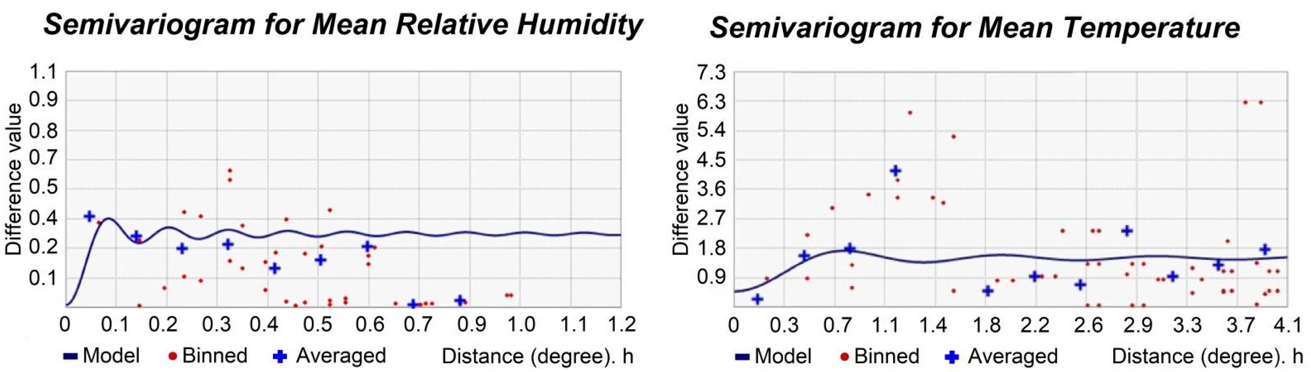
Best-fit models were chosen according to the semivariogram shape. In the semivariogram graph, measured values (PM
2.5, temperature or RH) are represented by red dots, and the mean values of those measured values are represented by blue crosses (
Figure 3,
Figure 4 and
Figure 5). Both variables were used for adjusting the model (represented as a continuous line) to the first measured and mean values in order to obtain a best fit. Those first measured values are related to each other when the distance is lower, as expressed by Tobler’s first law [
84]. For that purpose, a number of changes in the values and in the models can be carried out.
The first of the possibilities is the optimization of the values. Optimization is focused on the range of the semivariogram (the value in the
Y-axis where the semivariogram becomes stable) and uses the local polynomial interpolation to fit the model [
85]. Other possibilities include changing the values of the nugget and lag size until the best fit is approached.
The last step is modifying the search direction of the neighborhood. If the measured values have less spatial autocorrelation with the prediction location with less effect on the predicted value, these measures can be eliminated from the calculation of that particular prediction point by defining a search neighborhood.
In
Figure 3, the transformed histograms for mean temperature and mean relative humidity are shown, which were both adjusted to the best Gaussian shape.
Spatial trends for both temperature and RH were calculated as second-order polynomial distributions for three of the space orientations (North–South and West–East) and as a first-order polynomial distribution for one of the sides of the mean RH (West–East). A trend transformation or detrending was subsequently performed with respect to the higher order found on the three axes. A careful observation of the polynomials represented indicates that the lines begin at high values that decrease in trend, as there is a scrolling from south to north that increases as it moves west from the center of the domain in the case of mean temperature.
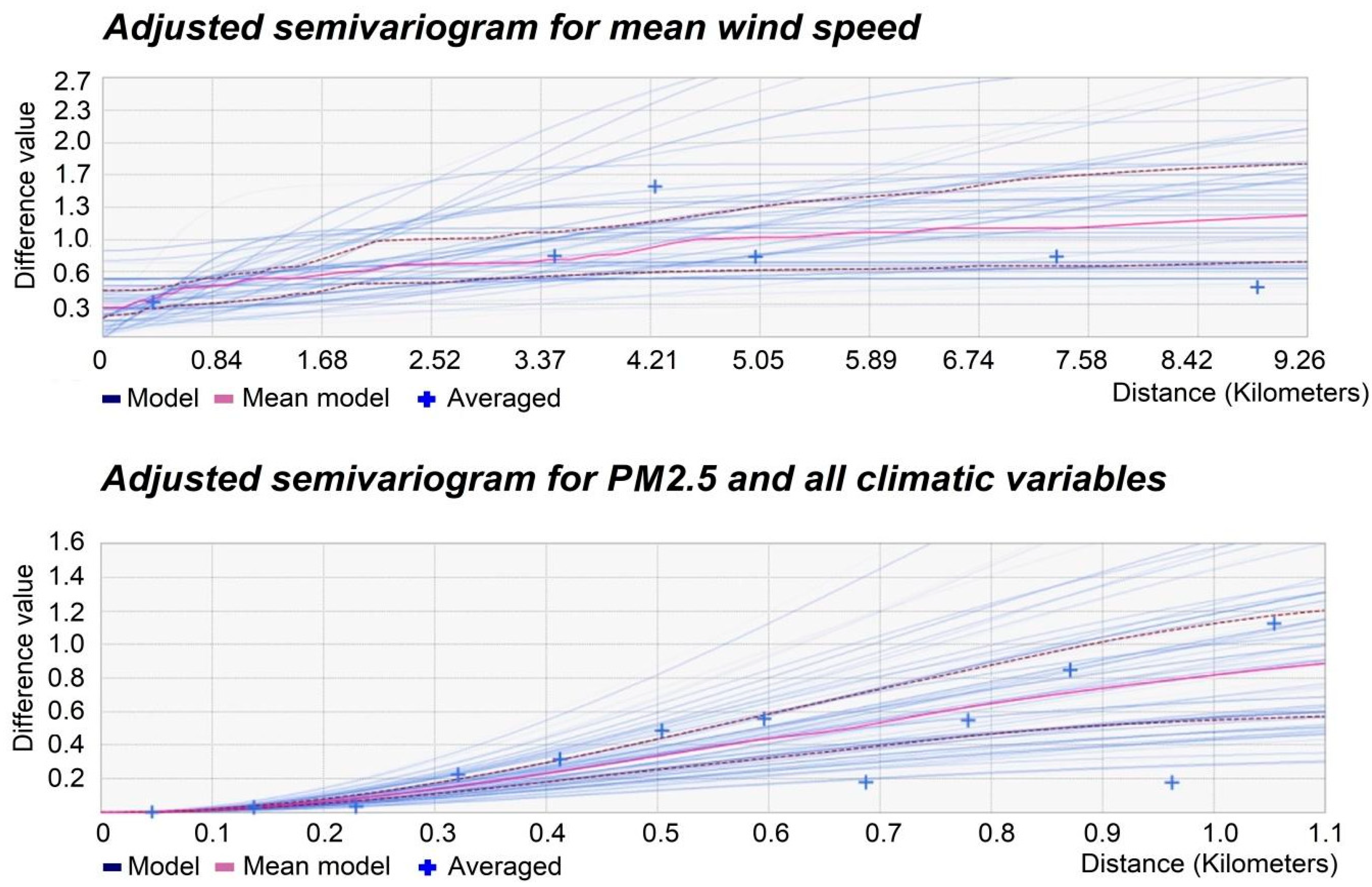
In
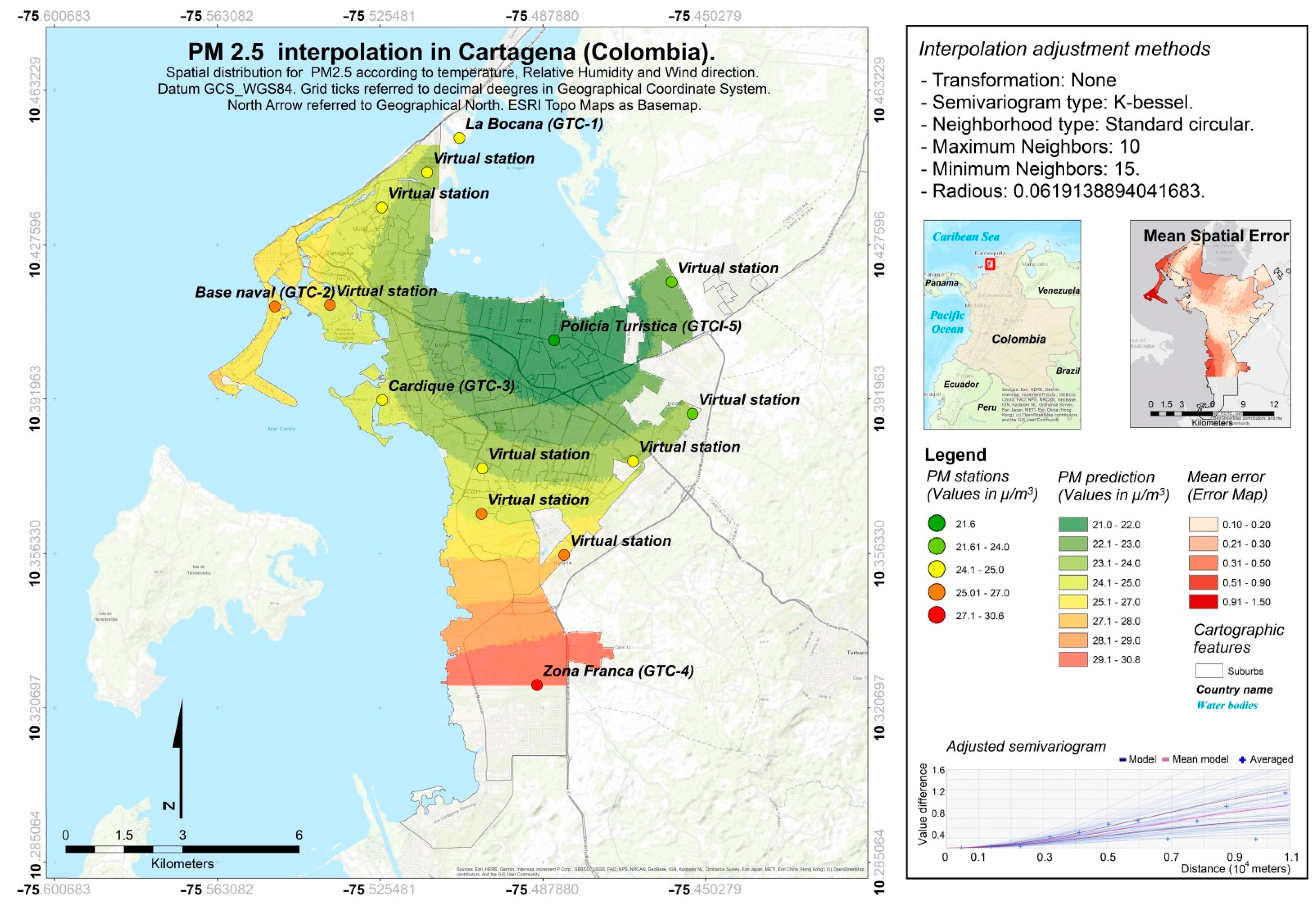
Figure 4, semivariograms with the adjusted functions using the EBK regression prediction for wind speed and PM
2.5 are shown, and in
Figure 5, the semivariograms corrected for mean temperature and mean RH are presented.
The first calculation of the estimated spatial error returned relatively acceptable values: they were only elevated in places remote from Cartagena. This error is smaller the closer it is to the value of 1, so high values (above 1) will have a lower reliability [
86]. The spatial error estimated values less than 4% in all cases, with the exception of the dry season RH, which had an error above 12%. Finally, the results were exported from a GA Layer format into a GRID format, and they were analyzed to provide a spatial mean calculation that could feed future health impact function analyses.
Results of the Interpolation of Weather Variables
Geostatistical interpolation analyses resolved up to nine different results considering each meteorological and PM
2.5 concentration variable, and one result more in the case of IDW. The following figures show the results in a mapping format for the top four variables of this study: mean PM
2.5 distribution (
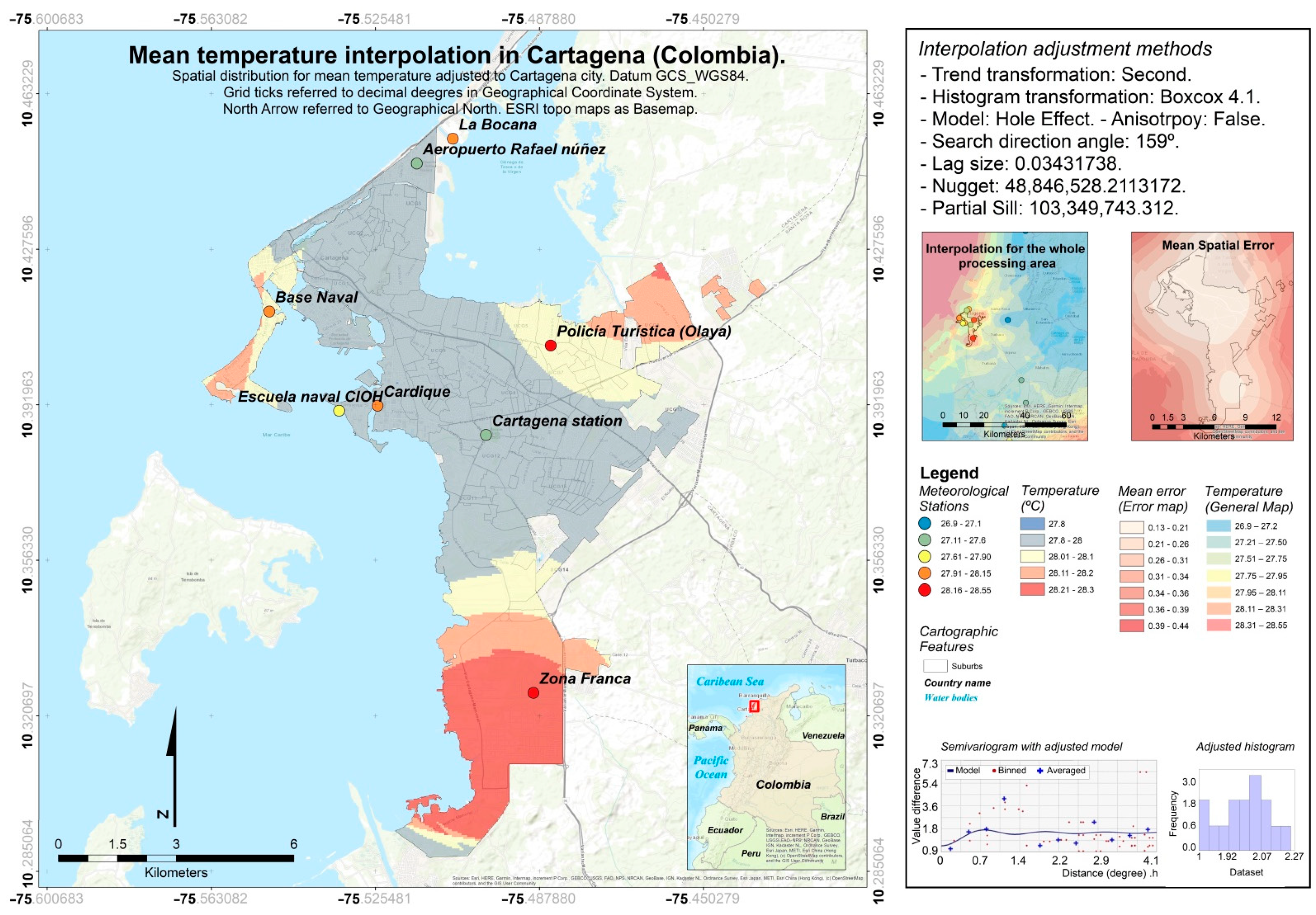
Figure 6), average temperature (
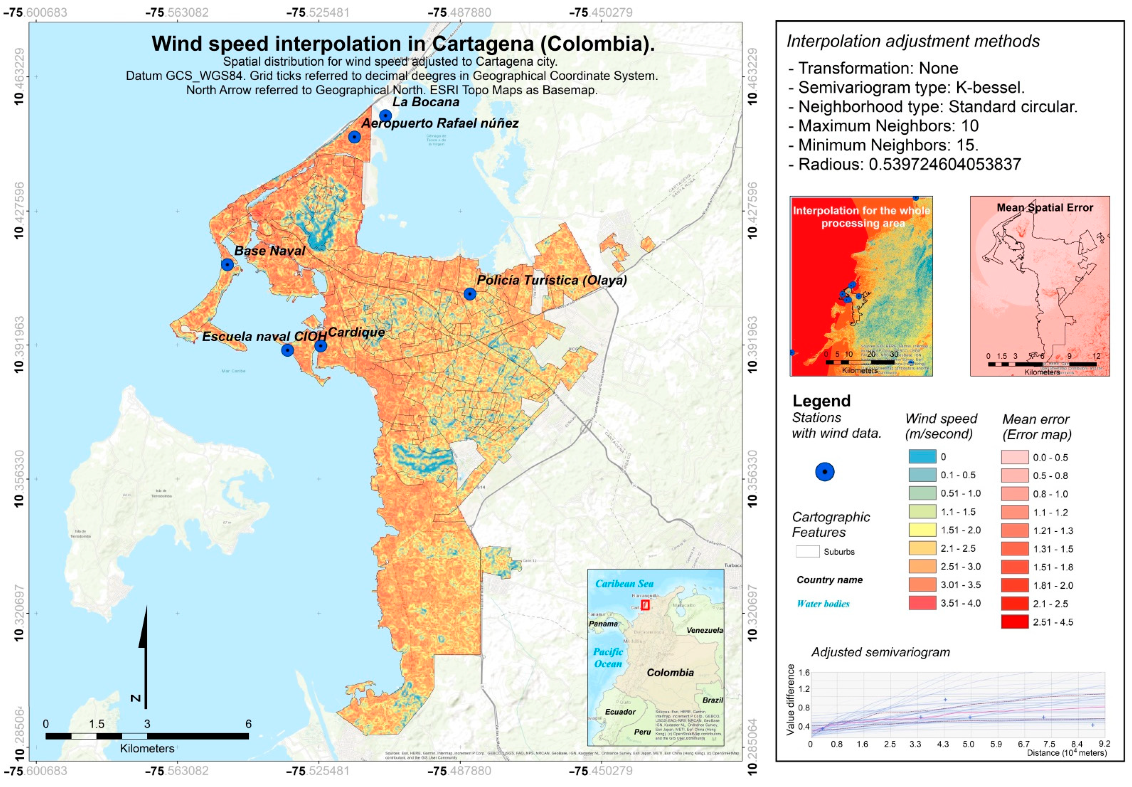
Figure 7), and wind speed (
Figure 8).
The rest of the interpolation results are presented in
Table 6, where some basic spatial statistics are adjusted to Cartagena. In turn, the arithmetic mean for each variable is displayed based on the data of all the stations analyzed. The latter value does not include the spatial weight granted by the interpolation.
In the case of mapping meteorological variables, it is possible to observe that RH and temperature parameters were found to be relatively stable and homogeneous throughout the city of Cartagena. The average temperature varied between 27.0 and 28.3 °C, with a slight difference of half a degree Celsius, which was mostly visible between the north and south of the city and between the center and the east and west distal areas. The mean spatial average was 28.01 °C for Cartagena, which was slightly greater than the mean derived from the data series. During the humid season, the spatial average equaled 28.22 °C, which was the same as the data series mean. Some differences were found in the temperature averages during the dry season, where the spatial mean equaled 27.84 °C, whereas the mean from the data series equaled 27.59 °C.
The average RH had the greatest differences among the values found in the city. However, its percentage expression indicates that the differences were also low. This may be indicative of some stability. Humidity in Cartagena seems to increase radially, from the center-west of the city to the north and south ends. The dynamic seems to be associated with its proximity to the open sea, the lowest humidity being in the center of the city due to the existence of the Tierra Bomba island, which blocks the entry of wet air towards Cartagena. In this study, values were found to range from 70.1% to 81%. Some differences can be found in the average spatial values, where the mean was situated at 75.34%, while the mean of the data series was greater at 76.89%. For the dry season, a slight difference of 0.26% was found in the comparison between the mean from the data series and the spatial mean, whereas during the wet season, up to 0.68 of a difference was found between the spatial mean and the data series mean. The wind speed average reached 2.3 m/s for the interpolation calculated, whereas according to the mean from the stations, the value was 1.56 m/s.
The interpolation of average PM2.5 presented a clear trend of reduction towards the north of the city. In turn, there were relatively high values in the area of Naval Base and Bocagrande. The high PM2.5 values recorded in the south of the city could have been a consequence of the industrial activity that is recorded in this area, whereas the high levels recorded in the northwest may have been due to port activity and the suspension of fine particles from beach areas.
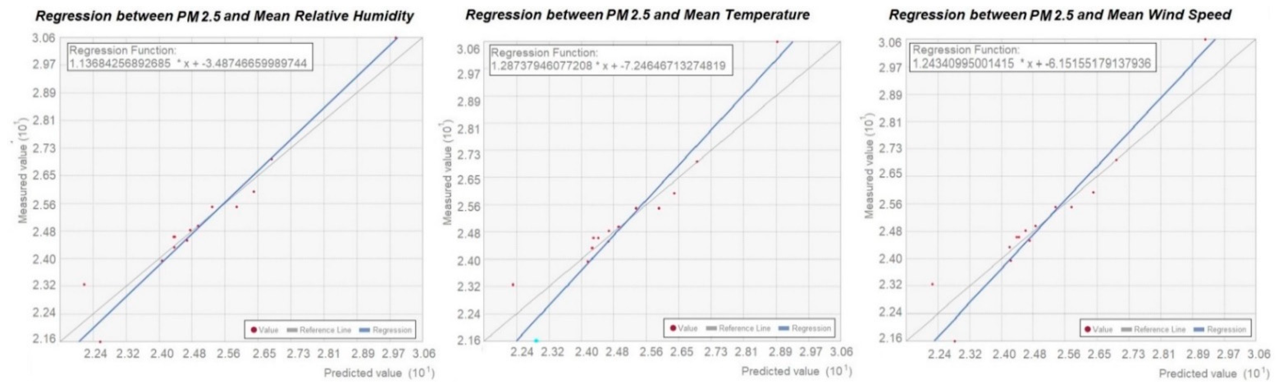
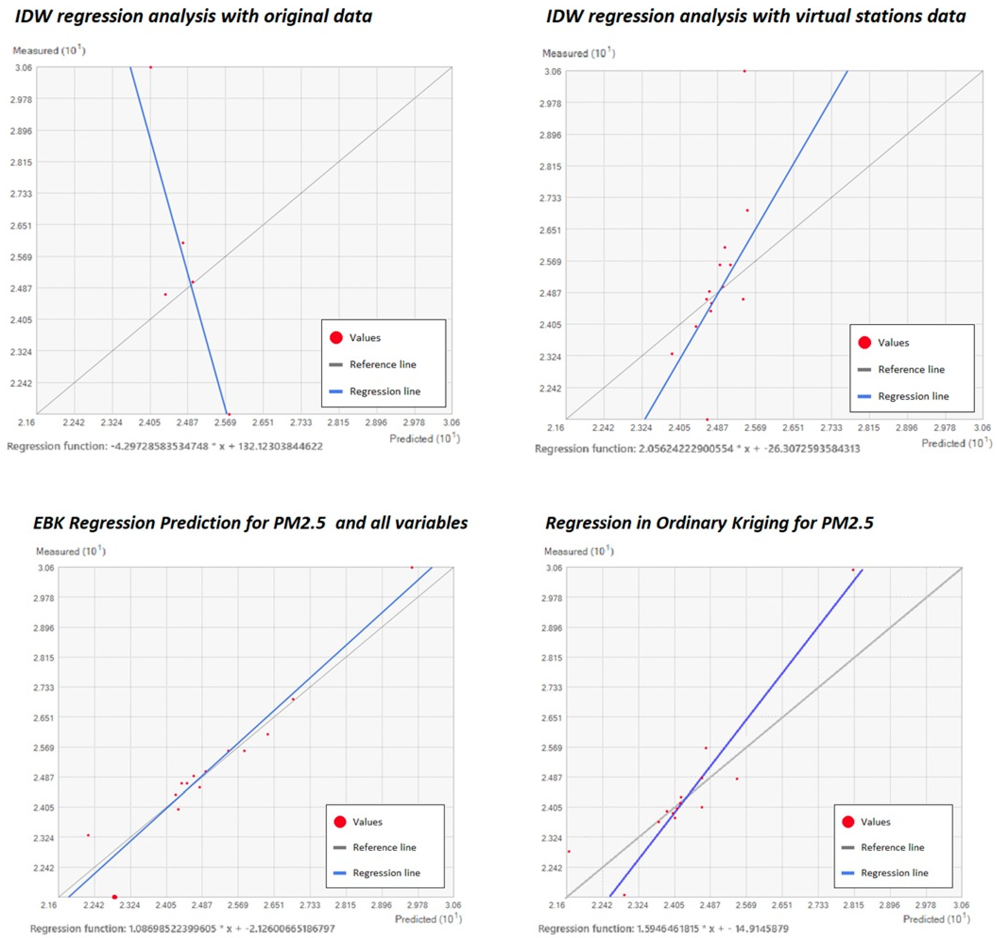
Regressions comparing PM
2.5 with each weather variable are shown in
Figure 9.
Regression analysis showed relative fitness for the spatial comparison between PM
2.5 and mean RH (
Figure 9) and slight fitness for the comparison between PM
2.5 and mean temperature (
Figure 9). Regression analysis also derived root mean square values, which were 0.64 in the case of PM
2.5—mean temperature, and 0–47 in the case of PM
2.5 and mean RH.
Regression analysis between PM
2.5 and mean wind speed is shown in
Figure 9. A slight correlation was found between these two parameters, with a root mean square value of 0.59 obtained.
The error between the measured and predicted values ranged from a maximum of 1.28 and a minimum of −0.14, and the standard error ranged from a maximum of 1.53 to a minimum of 0.19 (
Table 7).
For spatial errors derived from the spatial standard error maps of PM2.5, the interpolation showed major gaps in the northwestern side of the city (between Avenida Pedro Heredia and the southwestern corner of the Tesca Swamp) and to the southwest of Base Naval Station.
The mean errors for each interpolation method used in this study are shown in
Table 8.
When comparing the estimated errors, it can be observed that the method with the lowest error was EBK regression prediction, where the range of errors was between 1.2 and −1.01, and the mean of the estimated error was −0.10. The IDW interpolation method with virtual stations returned an error range of 3.43 to −1.14, with a mean of 1.60. The IDW method with the original stations (without the use of virtual stations) estimated an error of between 4.17 and −6.50, with a mean of 2.46. The ordinary kriging error ranged from 3.88 to −1.76, and the mean error was 0.79.
4. Discussion
The objective of this study was to estimate the PM2.5 concentrations at ground level and the continuous representation in space of essential weather variables. The application of geostatistical calculations led to a spatial characterization of the concentration levels of fine particles and of the temperature, wind direction and relative humidity meteorological variables in Cartagena, presenting a minimal error.
The spatial characterization at the maximum resolution of a particularly toxic pollutant, such as PM
2.5, is of great importance for exactly determining the exposed population in urban centers. In the specific case of Cartagena, it was determined that there are three areas that exceed the average concentration limits recommended by the World Health Organization [
87] for fine PM
2.5. Specifically, high PM
2.5 concentration levels were found, through interpolation, in the Base Naval, Centro district and Zona Franca areas. Although a physical–chemical study of fine particles was not conducted, it is assumed that the particle-generating elements are mainly road traffic and industrial activities, because there are no other combustion processes in the city or surrounding areas that may generate this pollutant.
In the case of meteorological variables, continuous temperature, wind speed and relative humidity values were obtained for the first time across the city of Cartagena. Temperature variability across the city was small, although a positive correlation between temperature and PM2.5 values was found. High PM2.5 values coincident with high temperature values were revealed again in the Zona Franca industry area, Centro district and in the Base Naval tourism sector.
Correlations between PM2.5 and wind speed, temperature and relative humidity showed the close influence of those meteorological variables on pollution in Cartagena, and allowed for the creation of highly accurate cartographic products for determining the distribution of PM2.5 in Cartagena de Indias.
As can be seen, the correlation between meteorological variables and PM
2.5 was found to be positive; therefore, a direct influence of these variables on the behavior of PM
2.5 was expected. Despite this supposed direct influence, the R
2 values did not reach values higher than 0.64. This could lead one to thinking that there must also be other variables that are influencing PM
2.5 concentrations. These variables could be the wind direction or the distribution of human activities throughout the city (industrial areas and main communication routes), factors that could not be measured in this study. However, it should be remembered that various investigations have found that the meteorological variables of wind speed, temperature and relative humidity exert both positive and negative influences [
88].
The positive influences of meteorological variables on PM
2.5 can range from the atmospheric stability on days of lower surface temperature [
89], periods of weak wind due to the presence of blocking anticyclones [
90], and the existence of PM
2.5 attached to water vapor during episodes of higher relative humidity [
22,
91], to the existence of PM
2.5 precursors due to greater photochemical reaction during temperature increases [
92,
93].
The negative influences of meteorological factors on PM
2.5 can reduce the spatial correlation and consequently cause a decrease in R
2. The negative influences of the meteorological variables on PM
2.5 can be higher temperature episodes that lead to greater turbulence and atmospheric convection [
94,
95], precipitation of PM
2.5 aggregates during increases in relative humidity above 70% [
22,
96], diffusion of PM
2.5 due to higher wind speed [
97,
98,
99,
100,
101,
102,
103,
104,
105,
106,
107,
108,
109,
110,
111] and higher evaporation-derived strong winds [
98].
In the specific case of Cartagena de Indias, it is possible that the variables that influence the positive relationship are the photochemical reactions due to higher temperatures and the accumulation of PM2.5 due to the low wind intensity. However, the existing high relative humidity (over 70%) may be forming aggregates of PM that precipitate by gravity processes or during rain episodes. In turn, PM2.5 may be reduced by the convective precipitation processes that are common on the Caribbean coast. The combination of all these specific influences would allow for the spatial correlation between PM2.5 and meteorological variables to be moderate, with values between 0.47 and 0.64 expected in the R2.
Some studies of pollutants in Cartagena de Indias found a low linear relationship between the same meteorological variables studied in this article and PM
2.5, and with other pollutants such as ozone or PM
10 [
34] determined that various environmental cofactors (such as humidity, temperature and wind dynamics) did not significantly modify concentrations of PM
2.5, or those of other atmospheric pollutants. These results are in contrast to those obtained in this analysis using the spatial and geostatistical correlation methods [
34].
Changes in meteorological variables have been found to exert a great influence on PM
2.5 levels. Xu et al. [
99] found that low wind speed, high relative humidity and low precipitation can lead to an increase of 29–42% of PM
2.5 in China. Zhao et al. [
21] also found that RH, precipitation and pressure were the most important variables for PM
2.5. They also found a good correlation between winter events and higher concentrations of PM
2.5, likely derived from heating devices and atmospheric stability. The results of these studies are in line with the main findings of this paper.
The characterization of PM
2.5 emissions throughout Cartagena has been measured in various studies [
100], corroborating the linkage of PM
2.5 with human activities and placing the highest concentrations in the industrial areas or near the main communication routes. Some technical reports of the environmental public body EPA-Cartagena [
28] analyzed the spatial distributions of PM
2.5 in the city, obtaining a general circular pattern of decreases in PM values near the Cardique station (in the west of the city), whereas to the south of the city, the highest concentrations were found. This distribution is in line with the results obtained in the present study, differing slightly when showing the minimum values of PM
2.5, which are located in the northeast of Cartagena.
Though the inverse distance weighting tool did not provide a spatial error estimation in ArcGis 10.5 or ArcGis Pro, the only possible evaluation of each method used was comparing the mean error and predicted values from the interpolation result.
When performing the interpolation with the IDW method and using the virtual stations, the predictive surface corresponding to average values (24–27 μg/m3) was found to increase, reducing the area represented for the lowest values (21–23 μg/m3) and higher ones (27–30 μg/m3). In the case of the IDW interpolation with original values, a large area with average values was also found, fundamentally to the west of the city, whereas the area with higher values, fundamentally to the south of the city (27–30 μg/m3), was found to increase.
The geostatistical approach in this study showed better results than deterministic (non-geostatistical) methods, as can be seen in the errors’ description in
Table 8 and
Figure 10. The lowest mean error and the lowest range of errors were achieved during the use of the EBK regression prediction tool and ordinary kriging. Therefore, technicians may find the geostatistical approach useful for pollutant interpolations. The reliability of the PM
2.5 interpolation method by the EBK regression prediction methodology can be specifically compared with the interpolation by ordinary kriging, where independent meteorological variables were not included. EBK regression prediction also showed more accurate results than ordinary kriging.
Since the error was also very small, it was decided to use the EBK-RP method due to its reduction in error by up to 0.69 points in comparison to ordinary kriging interpolation, or by up to 1.5 in comparison to IDW performed with virtual stations, as can be seen in
Table 8.
Certain studies consider that non-geostatistical methods, such as IDW, are an accurate technique for performing the interpolation of meteorological variables [
101], and also for particulate matter interpolations [
5].
However, some other investigations have determined the benefits of using kriging techniques instead of IDW due to lower spatial error results for pollutants [
102,
103,
104] or when interpolating meteorological variables [
101,
105].
Interpolation techniques which do not attempt to fit the data to a normal distribution can lead to interpolations with leptokurtic or platykurtic and left-scored histograms in the specific case of Cartagena. These types of distributions can lead to interpolations with discontinuities and so-called “bull-eyes” errors, meaning that no autocorrelation is achieved [
106]. These errors can be solved with a geostatistical approach.
Satellite remote sensing related to air quality is one of the methods that has been most developed in recent decades and is likely to be further developed in the coming years [
107]. Satellite images can provide an overview of the spatial distribution of PM
2.5 or of meteorological variables (excluding wind) with decameter precision. The main advantage of using satellite images is to obtain products with a spatially continuous distribution without the need for interpolation. Research in Colombia has found the measurement of NO
2 by satellite image to have a very good correlation (0.91) with ground stations [
108].
However, the satellite images used in this method do not have a temporal continuity, being only representations of an exact moment. Measurements at ground stations have the disadvantage of relying on spatial interpolation methods, but also the advantage of collecting measurements with greater temporal continuity.
In Cartagena de Indias, no specific air quality studies have been carried out using satellite images. Certain studies on the scale of the entire Colombian territory (with 1° resolution in latitude) found the Cartagena area to be one of the most polluted cities by PM
10 [
109], in addition to observing a relationship of this pollutant with vehicular traffic and anthropogenic activities. Other studies in the Bogotá area related 90% increases in PM
2.5 and PM
10 pollutants to the dry season [
110].
Some shortcomings could be pointed out from this study. Estimates of the values between points always have biases because of the sampling method. When the sampling network (in this case the ground stations) is not correctly distributed, over or under estimations could occur.
The distribution of PM2.5 in a city can increase locally due to the presence of certain urban elements, such as unvegetated vacant lots or highways with a high density of road traffic. If there are no stations near these urban elements, the PM may have estimation errors. An erroneous representation can also come from the proximity of a station to one of these elements, interpolating a PM2.5 value corresponding to a small space (such as a sand space without vegetation), which can become a generalized value for a larger space.
There may also be certain shortcomings when relating PM2.5 to meteorological variables. First, comparisons using unique data frames like those of this study can lead to errors by eliminating the comparison with daily variability, which is important for observing correlations in the increase or decrease in PM2.5 values and meteorological changes. Second, the absence of a meteorological network with homogenized data in Cartagena may prevent comparison with variables such as wind direction and may add errors by not allowing for comparisons with humidity and temperature variables during the same period.
Despite these limitations, the data analyzed in the case of Cartagena de Indias are the only data currently existing. It seems that the installation of new stations and the restarting of existing ones will not be taking place in the near future.
Due to the development of this study, improved values were obtained from the considered environmental variables that can be used to provide data to models of the impact of PM2.5 on human health. Estimating health impacts due to air pollutants is complicated in South America due to the absence of homogeneous series of data and the accuracy needed to define the dispersion of air pollutants, a task that may be facilitated through the use of spatial statistics techniques.
5. Conclusions
In this study, the spatial distribution of the pollutant PM2.5 in Cartagena de Indias, Colombia, was analyzed based on different spatial interpolation methods. An attempt to determine the existence of a positive correlation between the spatial distribution of PM2.5 and the spatial distribution of the meteorological variables of mean wind speed, mean temperature and mean relative humidity was undertaken.
Three areas of the city of Cartagena de Indias were found to exceed World Health Organization PM2.5 recommendations: the Zona Franca Industrial area, Centro district, and Base Naval tourism sector.
The relationships between PM2.5 and the meteorological variables showed a positive correlation, with moderately high R2 values. In turn, the relationship between PM2.5 and each variable separately provided estimates with an R2 of 0.47 for the correlation of PM2.5 and mean relative humidity, 0.59 for PM2.5 with mean wind speed, and 0.64 between the mean temperature and PM2.5.
EBK regression prediction proved to be the most accurate tool for obtaining results. The ordinary kriging tool can obtain results with a reduced error but without the possibility of adding independent variables in the estimates. Deterministic (non-geostatistical) methods, such as IDW, result in interpolations with a special representation similar to geostatistical methods, but with a greater error than these.
Therefore, the most reliable methods for mapping the PM2.5 pollutant in Cartagena are geostatistical methods.
Future studies may be related to comparisons between satellite images and PM ground measurements in Cartagena with meteorological variables on a daily scale. A better network for PM measurement, with a greater number of stations (outside and inside the city) and an hourly–daily time scale, is needed in Cartagena de Indias.

 ,
, 


