
Decomposition of Trend and Interdecadal Variation of Evaporation over the Tropical Indian Ocean in ERA5


Abstract
1. Introduction
2. Data and Methods
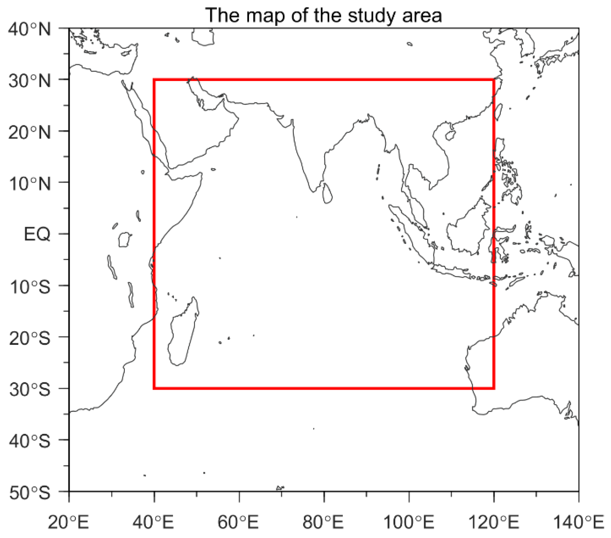
2.1. Data
2.2. Evaporation Decomposition Method
2.3. Statistical Methods
3. Results
3.1. Trend of Evaporation over the Tropical Indian Ocean
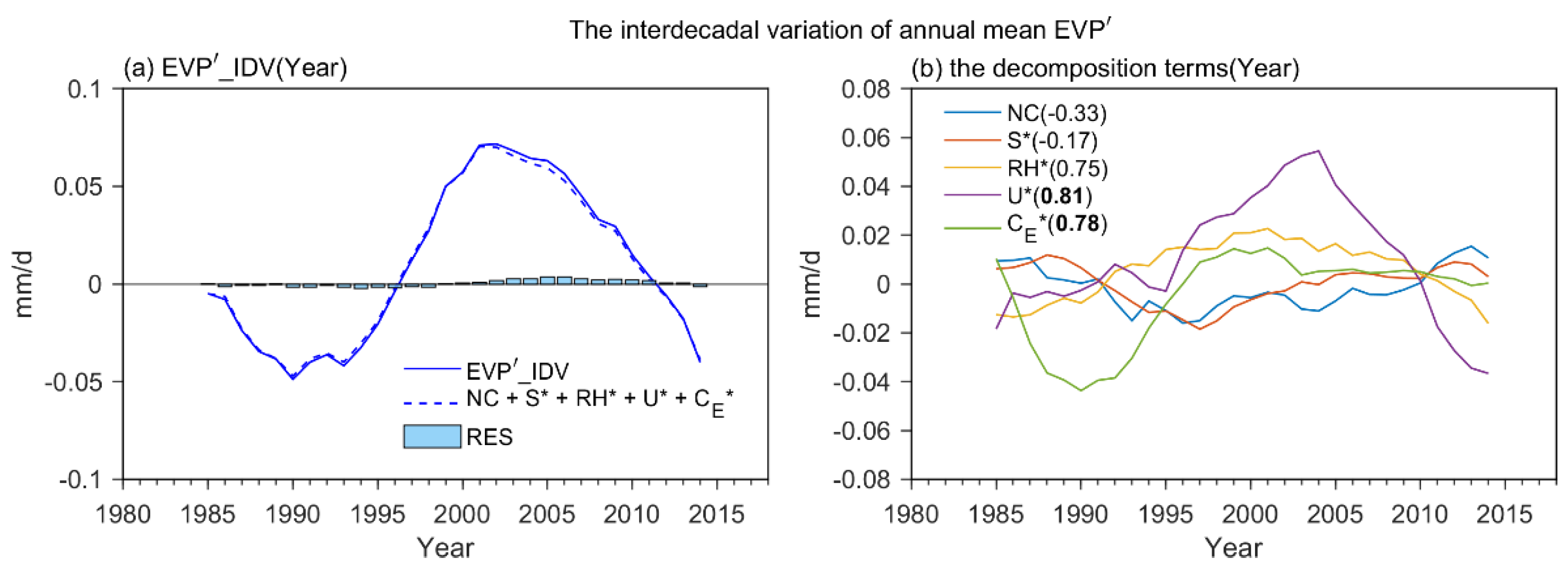
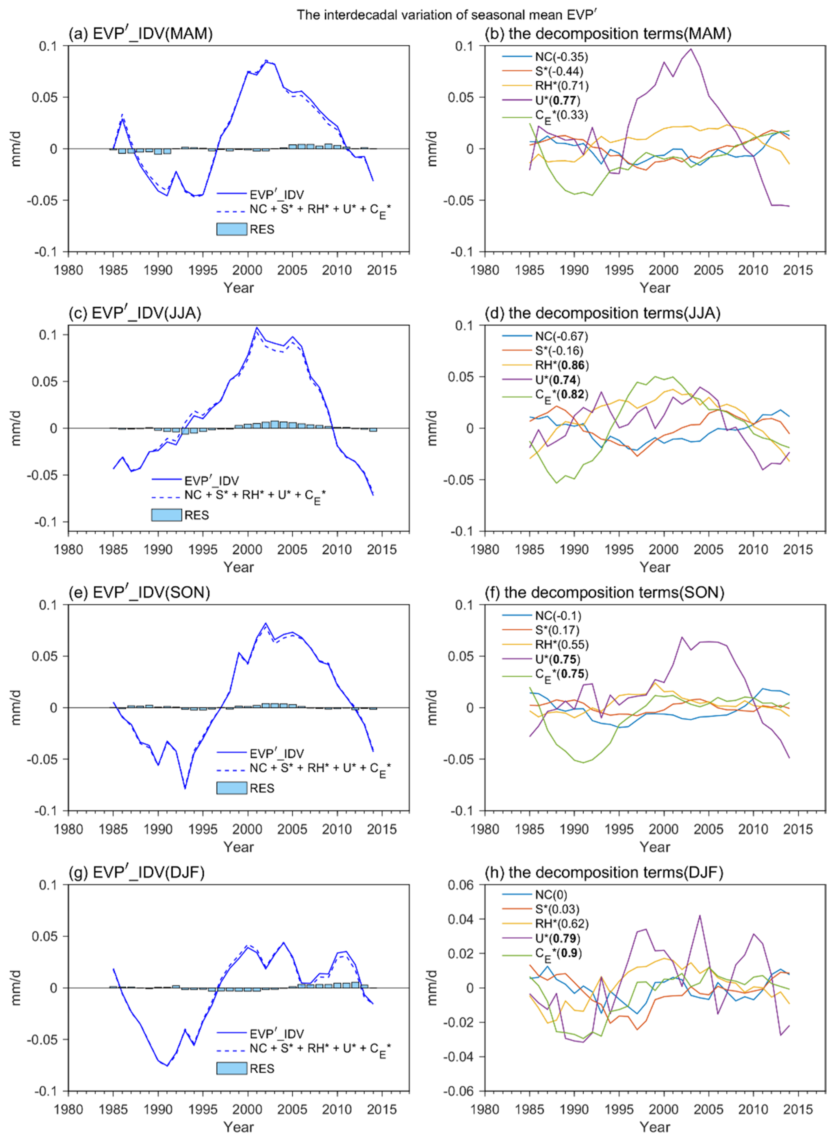
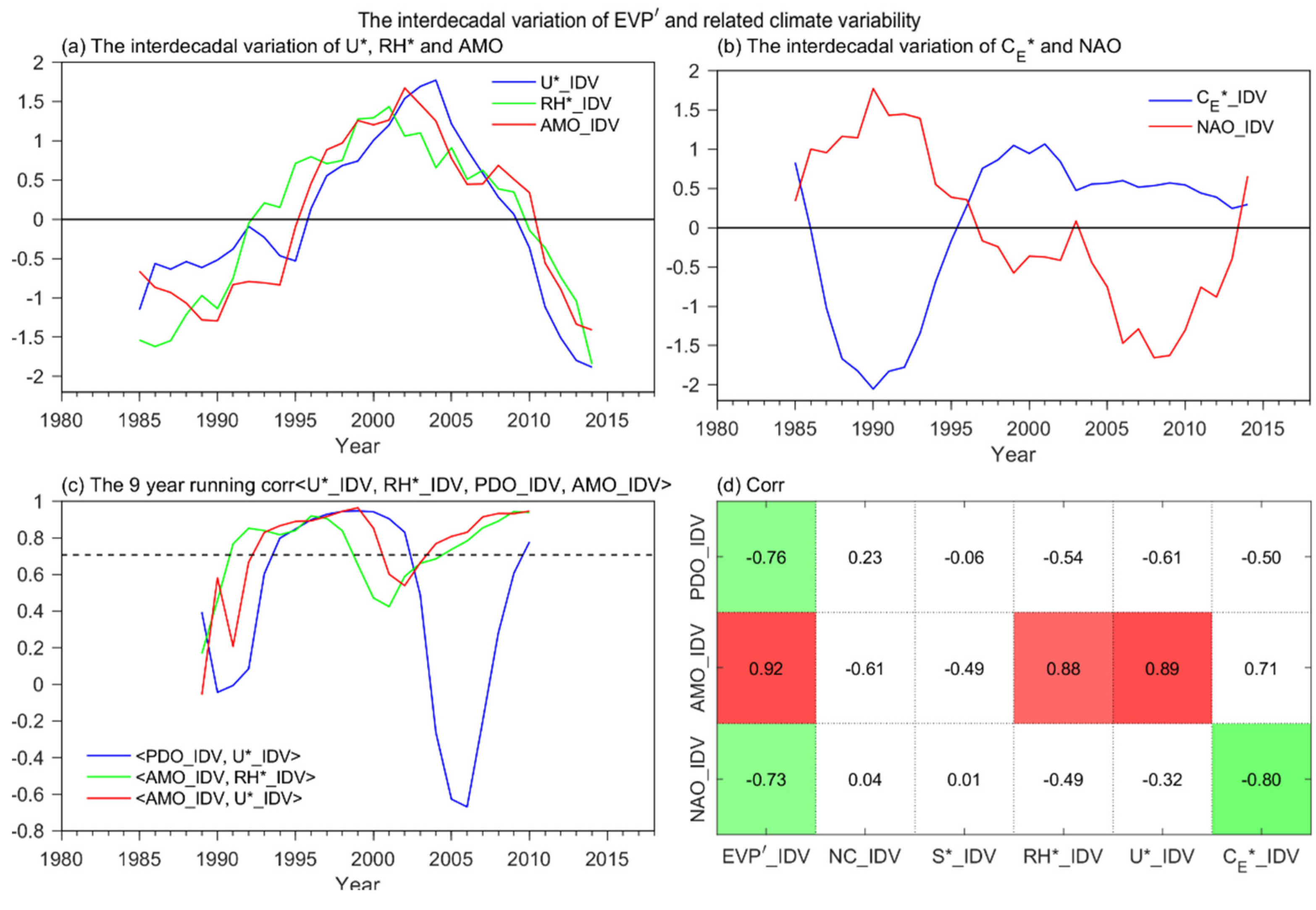
3.2. Interdecadal Variation of Evaporation over the Tropical Indian Ocean
4. Conclusions and Discussion
Author Contributions
Funding
Institutional Review Board Statement
Informed Consent Statement
Data Availability Statement
Conflicts of Interest
References
- Trenberth, K.E.; Caron, J.M.; Stepaniak, D.P. The atmospheric energy budget and implications for surface fluxes and ocean heat transports. Clim. Dyn. 2001, 17, 259–276. [Google Scholar] [CrossRef]
- Valdivieso, M.; Haines, K.; Balmaseda, M.; Chang, Y.-S.; Drevillon, M.; Ferry, N.; Fujii, Y.; Köhl, A.; Storto, A.; Toyoda, T.; et al. An assessment of air–sea heat fluxes from ocean and coupled reanalyses. Clim. Dyn. 2017, 49, 983–1008. [Google Scholar] [CrossRef]
- Kumar, B.P.; Cronin, M.F.; Joseph, S.; Ravichandran, M.; Sureshkumar, N. Latent Heat Flux Sensitivity to Sea Surface Temperature: Regional Perspectives. J. Clim. 2017, 30, 129–143. [Google Scholar] [CrossRef]
- Wang, C.; Weisberg, R.H.; Yang, H. Effects of the Wind Speed–Evaporation–SST Feedback on the El Niño–Southern Oscillation. J. Atmos. Sci. 1999, 56, 1391–1403. [Google Scholar] [CrossRef]
- Yu, L.; Jin, X.; Josey, S.A.; Lee, T.; Kumar, A.; Wen, C.; Xue, Y. The global ocean water cycle in atmospheric reanalysis, satellite, and ocean salinity. J. Clim. 2017, 30, 3829–3852. [Google Scholar] [CrossRef]
- Cayan, D.R. Latent and Sensible Heat Flux Anomalies over the Northern Oceans: Driving the Sea Surface Temperature. J. Phys. Oceanogr. 1992, 22, 859–881. [Google Scholar] [CrossRef]
- Alory, G.; Wijffels, S.; Meyers, G. Observed temperature trends in the Indian Ocean over 1960–1999 and associated mechanisms. Geophys. Res. Lett. 2007, 34, L02606. [Google Scholar] [CrossRef]
- Du, Y.; Xie, S.-P. Role of atmospheric adjustments in the tropical Indian Ocean warming during the 20th century in climate models. Geophys. Res. Lett. 2008, 35, L08712. [Google Scholar] [CrossRef]
- Chen, X.; Yao, Y.; Zhao, S.; Li, Y.; Jia, K.; Zhang, X.; Shang, K.; Xu, J.; Bei, X. Estimation of High-Resolution Global Monthly Ocean Latent Heat Flux from MODIS SST Product and AMSR-E Data. Adv. Meteorol. 2020, 2020. [Google Scholar] [CrossRef]
- Zeng, L.; Shi, P.; Liu, W.T.; Wang, D. Evaluation of a satellite-derived latent heat flux product in the South China Sea: A comparison with moored buoy data and various products. Atmos. Res. 2009, 94, 91–105. [Google Scholar] [CrossRef]
- Bourras, D. Comparison of Five Satellite-Derived Latent Heat Flux Products to Moored Buoy Data. J. Clim. 2006, 19, 6291–6313. [Google Scholar] [CrossRef]
- Hegerl, G.C.; Black, E.; Allan, R.P.; Ingram, W.J.; Polson, D.; Trenberth, K.E.; Chadwick, R.S.; Arkin, P.A.; Sarojini, B.B.; Becker, A.; et al. Challenges in Quantifying Changes in the Global Water Cycle. Bull. Am. Meteorol. Soc. 2015, 96, 1097–1115. [Google Scholar] [CrossRef]
- Kang, S.; Ahn, J.-B. Global energy and water balances in the latest reanalyses. Asia-Pac. J. Atmos. Sci. 2015, 51, 293–302. [Google Scholar] [CrossRef]
- Liu, J.; Curry, J.A. Variability of the tropical and subtropical ocean surface latent heat flux during 1989–2000. Geophys. Res. Lett. 2006, 33, L05706. [Google Scholar] [CrossRef]
- Li, G.; Ren, B.; Yang, C.; Zheng, J. Revisiting the trend of the tropical and subtropical Pacific surface latent heat flux during 1977–2006. J. Geophys. Res. Atmos. 2011, 116, D10115. [Google Scholar] [CrossRef]
- Gao, S.; Chiu, L.S.; Shie, C.-L. Trends and variations of ocean surface latent heat flux: Results from GSSTF2c data set. Geophys. Res. Lett. 2013, 40, 380–385. [Google Scholar] [CrossRef]
- Pokhrel, S.; Dutta, U.; Rahaman, H.; Chaudhari, H.; Hazra, A.; Saha, S.K.; Veeranjaneyulu, C. Evaluation of Different Heat Flux Products Over the Tropical Indian Ocean. Earth Space Sci. 2020, 7, e2019EA000988. [Google Scholar] [CrossRef]
- Liu, W.T.; Katsaros, K.B.; Businger, J.A. Bulk Parameterization of Air-Sea Exchanges of Heat and Water Vapor Including the Molecular Constraints at the Interface. J. Atmos. Sci. 1979, 36, 1722–1735. [Google Scholar] [CrossRef]
- Richter, I.; Xie, S.-P. Muted precipitation increase in global warming simulations: A surface evaporation perspective. J. Geophys. Res. 2008, 113, D24118. [Google Scholar] [CrossRef]
- Wu, R.; Kirtman, B.P.; Pegion, K. Local Air–Sea Relationship in Observations and Model Simulations. J. Clim. 2006, 19, 4914–4932. [Google Scholar] [CrossRef]
- Lorenz, D.J.; DeWeaver, E.T.; Vimont, D.J. Evaporation Change and Global Warming: The Role of Net Radiation and Relative Humidity. J. Geophys. Res. 2010, 115, D20118. [Google Scholar] [CrossRef]
- Yu, L. Global Variations in Oceanic Evaporation (1958–2005): The Role of the Changing Wind Speed. J. Clim. 2007, 20, 5376–5390. [Google Scholar] [CrossRef]
- Xie, S.-P.; Philander, S.G.H. A coupled ocean-atmosphere model of relevance to the ITCZ in the eastern Pacific. Tellus A 1994, 46, 340–350. [Google Scholar] [CrossRef]
- Zhou, X.; Ray, P.; Barrett, B.S.; Hsu, P.-C. Understanding the bias in surface latent and sensible heat fluxes in contemporary AGCMs over tropical oceans. Clim. Dyn. 2020, 55, 2957–2978. [Google Scholar] [CrossRef]
- Robertson, F.R.; Bosilovich, M.G.; Roberts, J.B.; Reichle, R.H.; Adler, R.; Ricciardulli, L.; Berg, W.; Huffman, G.J. Consistency of Estimated Global Water Cycle Variations over the Satellite Era. J. Clim. 2014, 27, 6135–6154. [Google Scholar] [CrossRef][Green Version]
- Bosilovich, M.G.; Robertson, F.R.; Takacs, L.; Molod, A.; Mocko, D. Atmospheric Water Balance and Variability in the MERRA-2 Reanalysis. J. Clim. 2017, 30, 1177–1196. [Google Scholar] [CrossRef]
- Hersbach, H.; Bell, B.; Berrisford, P.; Hirahara, S.; Horányi, A.; Muñoz-Sabater, J.; Nicolas, J.; Peubey, C.; Radu, R.; Schepers, D.; et al. The ERA5 global reanalysis. Q. J. R. Meteorol. Soc. 2020, 146, 1999–2049. [Google Scholar] [CrossRef]
- Huang, B.; Thorne, P.W.; Banzon, V.F.; Boyer, T.; Chepurin, G.; Lawrimore, J.H.; Menne, M.J.; Smith, T.M.; Vose, R.S.; Zhang, H.-M. Extended Reconstructed Sea Surface Temperature, Version 5 (ERSSTv5): Upgrades, Validations, and Intercomparisons. J. Clim. 2017, 30, 8179–8205. [Google Scholar] [CrossRef]
- Pyper, B.J.; Peterman, R.M. Comparison of methods to account for autocorrelation in correlation analyses of fish data. Can. J. Fish. Aquat. Sci. 1998, 55, 2127–2140. [Google Scholar] [CrossRef]
- Li, J.; Sun, C.; Jin, F.F. NAO implicated as a predictor of Northern Hemisphere mean temperature multidecadal variability. Geophys. Res. Lett. 2013, 40, 5497–5502. [Google Scholar] [CrossRef]
- Cao, N.; Ren, B. Regime shift of global oceanic evaporation in the late 1990s using OAFlux dataset. Theor. Appl. Climatol. 2019, 136, 1407–1417. [Google Scholar] [CrossRef]
- Tao, W.; Huang, G.; Hu, K.; Qu, X.; Wen, G.; Gong, H. Interdecadal modulation of ENSO teleconnections to the Indian Ocean Basin Mode and their relationship under global warming in CMIP5 models. Int. J. Climatol. 2015, 35, 391–407. [Google Scholar] [CrossRef]
- Young, I.R.; Zieger, S.; Babanin, A.V. Global trends in wind speed and wave height. Science 2011, 332, 451–455. [Google Scholar] [CrossRef] [PubMed]
- Li, G.; Ren, B. Evidence for strengthening of the tropical Pacific Ocean surface wind speed during 1979–2001. Theor. Appl. Climatol. 2012, 107, 59–72. [Google Scholar] [CrossRef]
- Li, X.; Xie, S.P.; Gille, S.T.; Yoo, C. Atlantic-induced pan-tropical climate change over the past three decades. Nat. Clim. Chang. 2016, 6, 275–279. [Google Scholar] [CrossRef]
- Jin, X.; Kwon, Y.O.; Ummenhofer, C.C.; Seo, H.; Schwarzkopf, F.U.; Biastoch, A.; Böning, C.W.; Wright, J.S. Influences of pacific climate variability on decadal subsurface Ocean heat content variations in the Indian Ocean. J. Clim. 2018, 31, 4157–4174. [Google Scholar] [CrossRef]
- Morioka, Y.; Tozuka, T.; Masson, S.; Terray, P.; Luo, J.-J.; Yamagata, T. Subtropical Dipole Modes Simulated in a Coupled General Circulation Model. J. Clim. 2012, 25, 4029–4047. [Google Scholar] [CrossRef]


| NC | S* | RH* | U* | CE* | ||
|---|---|---|---|---|---|---|
| Year | 0.085 | 0.026 | −0.004 | 0.031 | 0.026 | 0.001 |
| MAM | 0.098 | 0.022 | 0 | 0.035 | 0.034 | 0.004 |
| JJA | 0.081 | 0.03 | 0.003 | 0.036 | 0.01 | 0.002 |
| SON | 0.078 | 0.027 | −0.014 | 0.021 | 0.029 | 0.013 |
| DJF | 0.086 | 0.025 | −0.006 | 0.032 | 0.033 | 0.001 |
Publisher’s Note: MDPI stays neutral with regard to jurisdictional claims in published maps and institutional affiliations. |
© 2022 by the authors. Licensee MDPI, Basel, Switzerland. This article is an open access article distributed under the terms and conditions of the Creative Commons Attribution (CC BY) license (https://creativecommons.org/licenses/by/4.0/).
Share and Cite
Huang, B.; Su, T.; Zhang, Z.; Wu, Y.; Feng, G. Decomposition of Trend and Interdecadal Variation of Evaporation over the Tropical Indian Ocean in ERA5. Atmosphere 2022, 13, 496. https://doi.org/10.3390/atmos13030496
Huang B, Su T, Zhang Z, Wu Y, Feng G. Decomposition of Trend and Interdecadal Variation of Evaporation over the Tropical Indian Ocean in ERA5. Atmosphere. 2022; 13(3):496. https://doi.org/10.3390/atmos13030496
Chicago/Turabian StyleHuang, Bicheng, Tao Su, Zengping Zhang, Yongping Wu, and Guolin Feng. 2022. "Decomposition of Trend and Interdecadal Variation of Evaporation over the Tropical Indian Ocean in ERA5" Atmosphere 13, no. 3: 496. https://doi.org/10.3390/atmos13030496
APA StyleHuang, B., Su, T., Zhang, Z., Wu, Y., & Feng, G. (2022). Decomposition of Trend and Interdecadal Variation of Evaporation over the Tropical Indian Ocean in ERA5. Atmosphere, 13(3), 496. https://doi.org/10.3390/atmos13030496