
Analysis of Wildfires in the Mid and High Latitudes Using a Multi-Dataset Approach: A Case Study in California and Krasnoyarsk Krai


Abstract
:1. Introduction
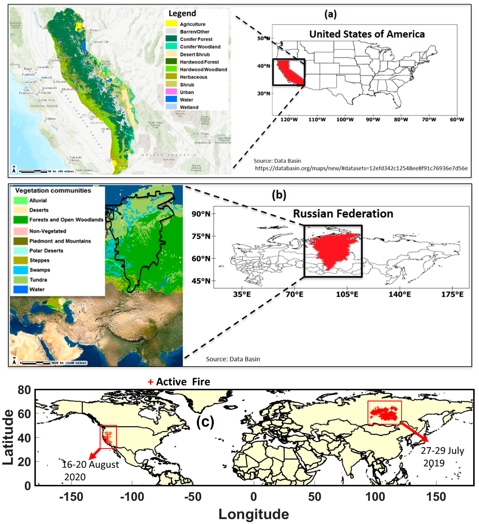
2. Study Areas
3. Data
3.1. Cloud-Aerosol LiDAR and Infrared Pathfinder Satellite Observations (CALIPSO)
3.2. Sentinel-5P (TROPOMI)
3.3. Moderate-Resolution Imaging Spectroradiometer (MODIS)
3.4. Modern-Era Retrospective Analysis for Research and Applications Version 2 (MERRA-2)
3.5. Hybrid Single-Particle Lagrangian Integrated Trajectory Model (HYSPLIT)
4. Results and Discussion
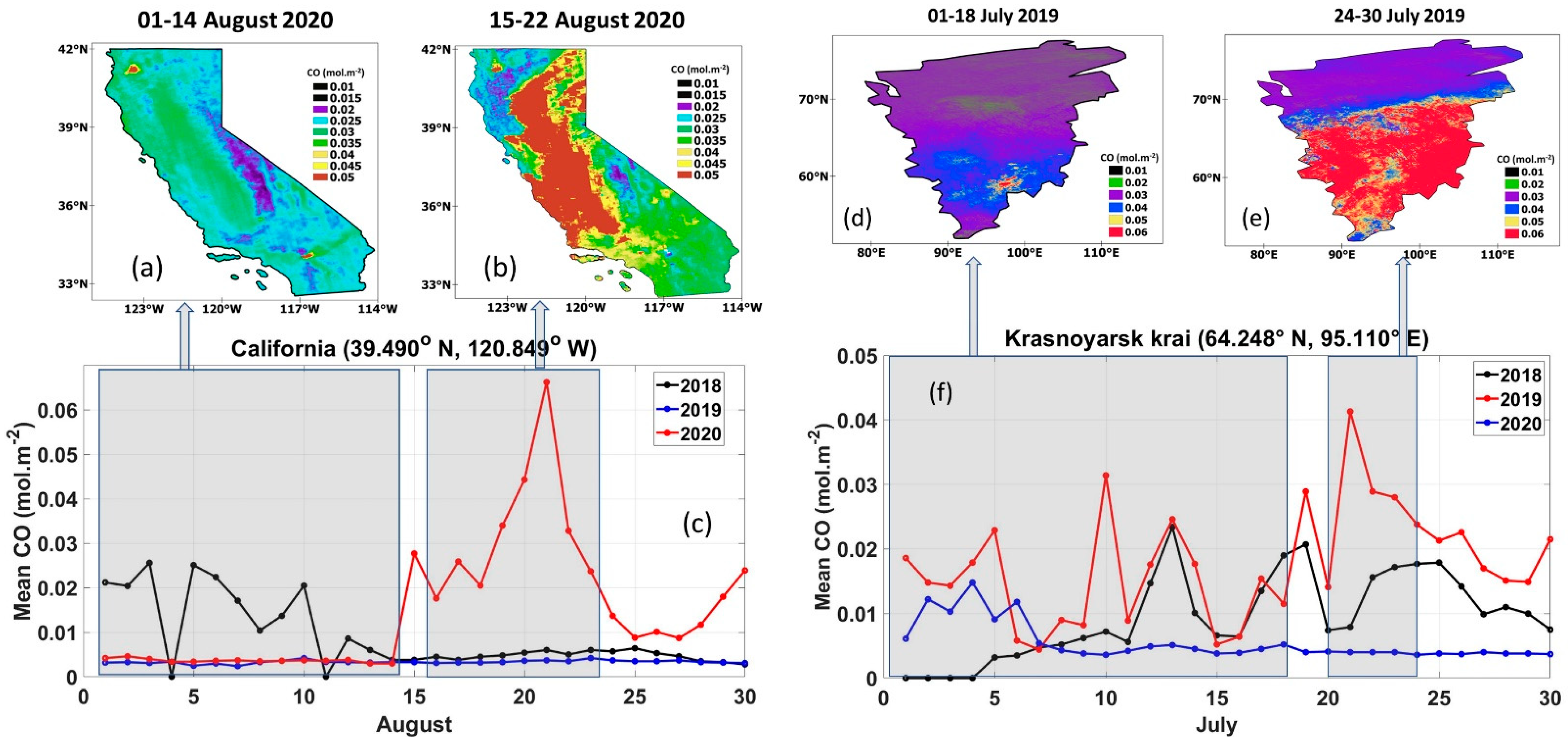
4.1. TROPOMI CO Observation
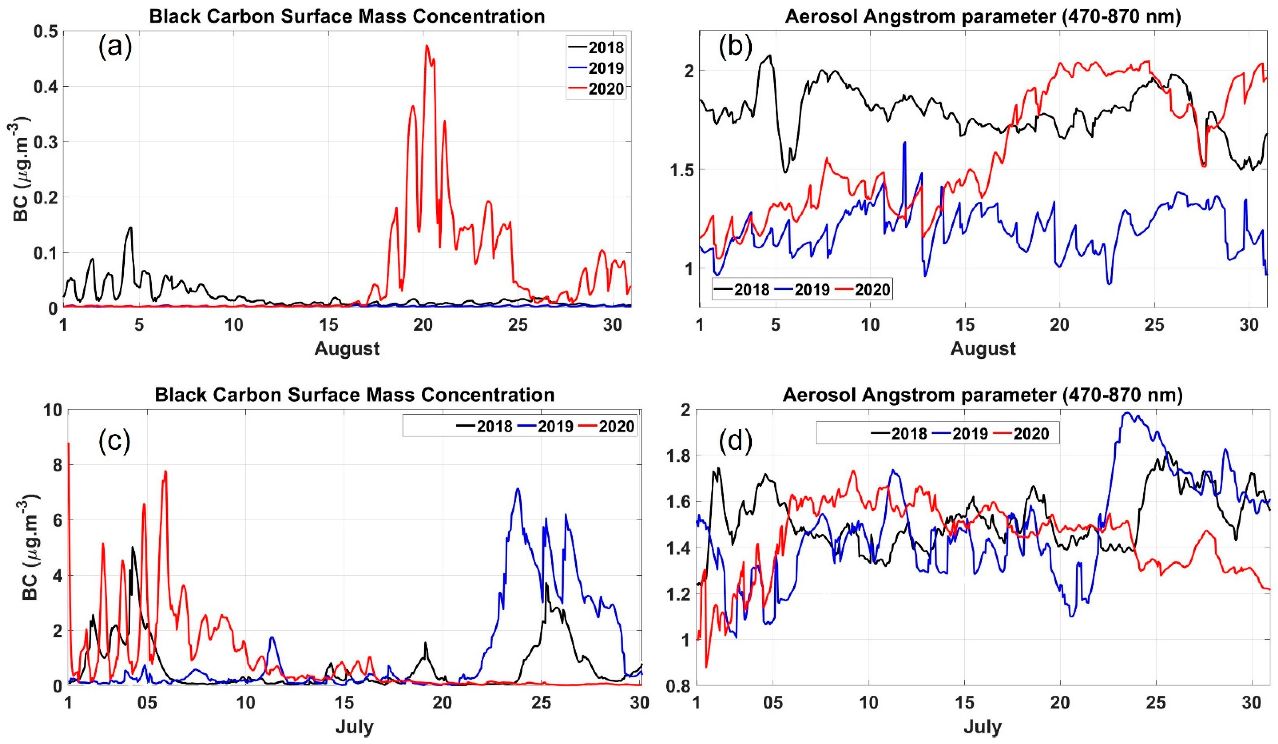
4.2. BC and AAP Timeseries
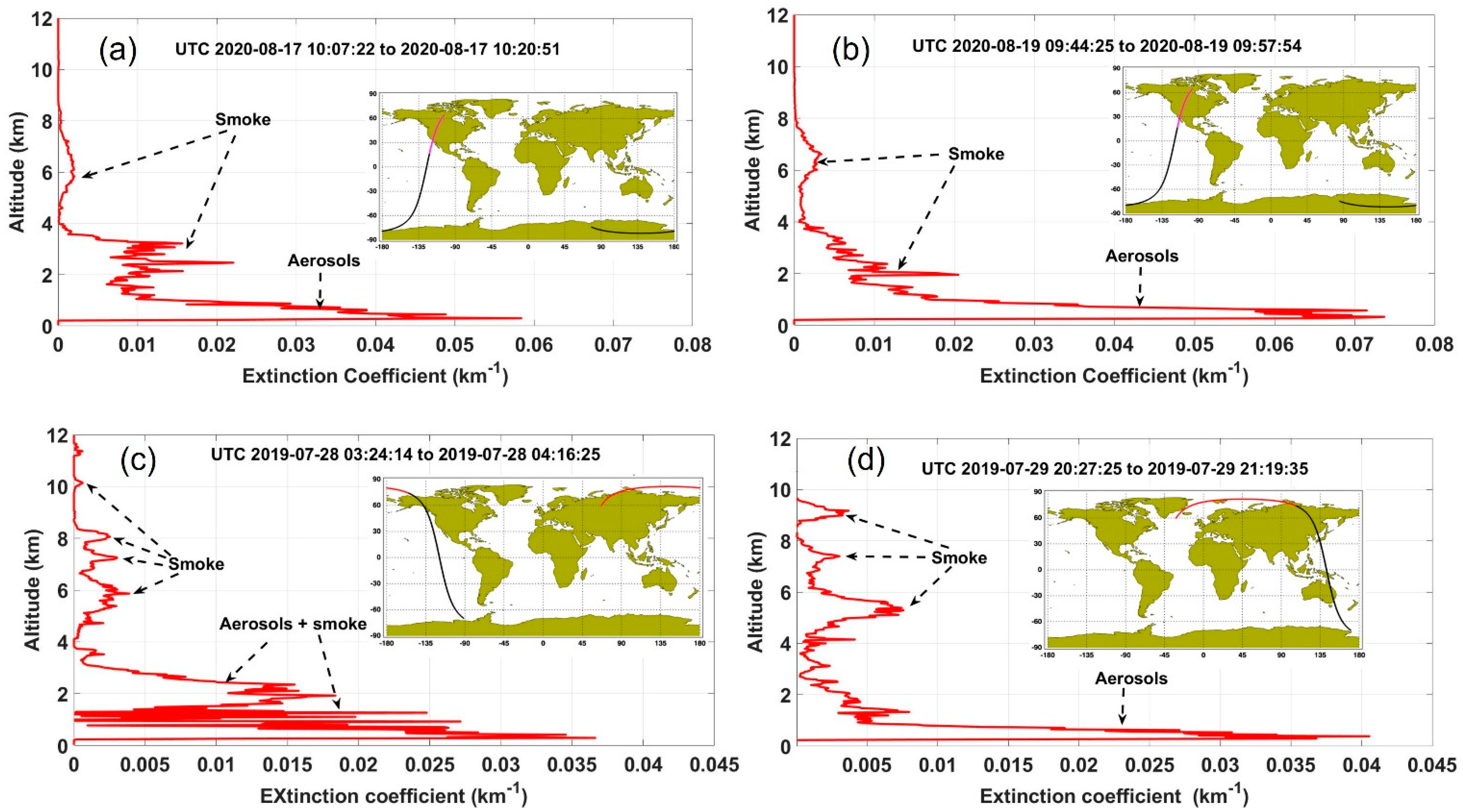
4.3. CALIOP Aerosol Extinction Coefficient Vertical Height Profiles
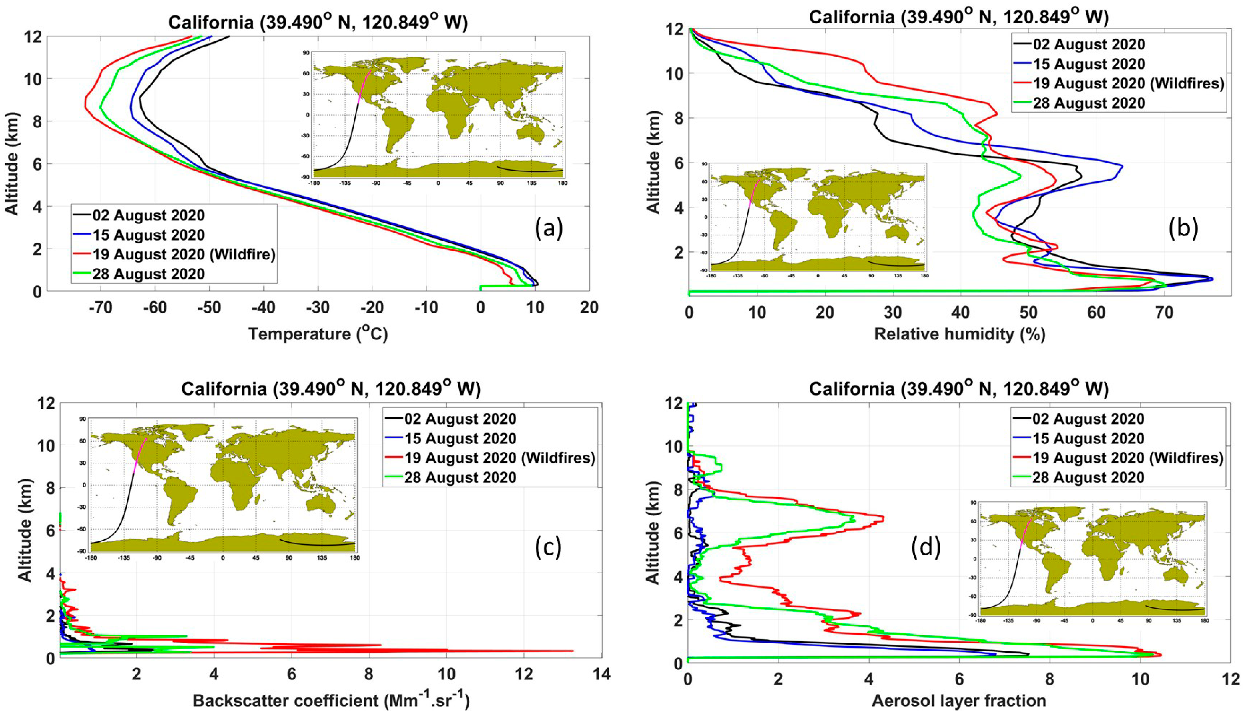
4.4. Temperature, Relative Humidity, Backscatter Coefficient and Aerosol Layer Profiles
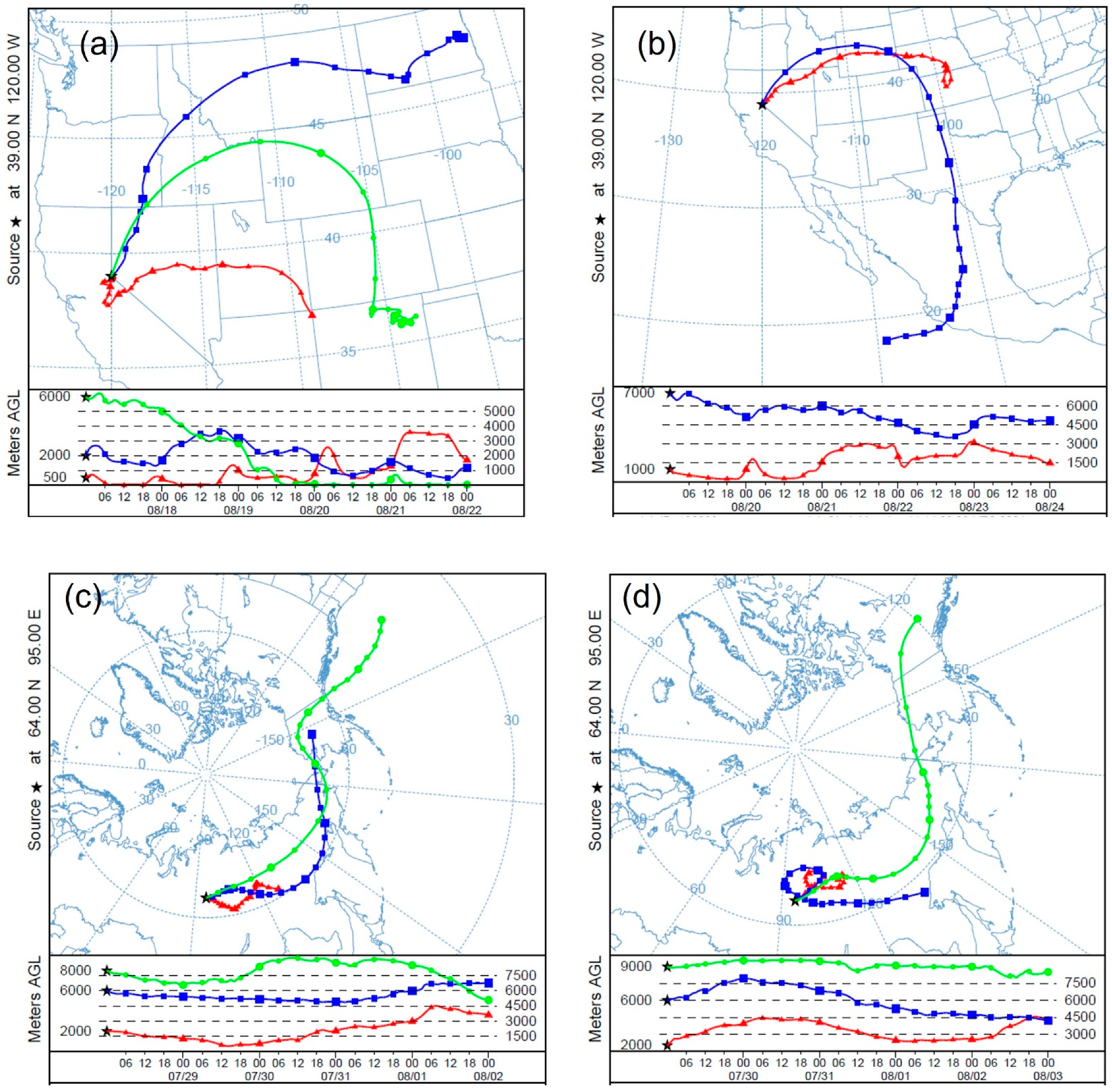
4.5. Transport of the Pollutants
5. Conclusions
Author Contributions
Funding
Institutional Review Board Statement
Informed Consent Statement
Data Availability Statement
Acknowledgments
Conflicts of Interest
References
- Pyne, S.J.; Andrews, P.L.; Laven, R.D. Introduction to Wildland Fire; John Wiley & Sons: New York, NY, USA, 1996; 769p. [Google Scholar]
- Bodí, M.B.; Martin, D.A.; Balfour, V.N.; Santín, C.; Doerr, S.H.; Pereira, P.; Cerdà, A.; Mataix-Solera, J. Wildland fire ash: Production, composition and eco-hydro-geomorphic effects. Earth Sci. Rev. 2014, 130, 103–127. [Google Scholar] [CrossRef]
- Miller, J.D.; Yool, S.R. Mapping forest post-fire canopy consumption in several overstory types using multi-temporal Landsat TM and ETM data. Remote Sens. Environ. 2002, 82, 481–496. [Google Scholar] [CrossRef]
- Ruffault, J.; Curt, T.; Moron, V.; Trigo, R.M.; Mouillot, F.; Koutsias, N.; Pimont, F.; Martin-St Paul, N.; Barbero, R.; Dupuy, J.-L.; et al. Increased likelihood of heat-induced large wildfires in the Mediterranean Basin. Sci. Rep. 2020, 10, 13790. [Google Scholar] [CrossRef]
- Littell, J.S.; McKenzie, D.; Peterson, D.L.; Westerling, A.L. Climate and wildfire area burned in western U.S. ecoprovinces, 1916–2003. Ecol. Appl. 2009, 19, 1003–1021. [Google Scholar] [CrossRef]
- Barbero, R.; Abatzoglou, J.T.; Kolden, C.A.; Hegewisch, K.C.; Larkin, N.K.; Podschwit, H. Multi-scalar influence of weather and climate on very large-fires in the Eastern United States. Int. J. Clim. 2015, 35, 2180–2186. [Google Scholar] [CrossRef]
- Jiang, Y.; Yang, X.-Q.; Liu, X.; Qian, Y.; Zhang, K.; Wang, M.; Li, F.; Wang, Y.; Lu, Z. Impacts of Wildfire Aerosols on Global Energy Budget and Climate: The Role of Climate Feedbacks. J. Clim. 2020, 33, 3351–3366. [Google Scholar] [CrossRef]
- Kganyago, M.; Shikwambana, L. Assessment of the Characteristics of Recent Major Wildfires in the USA, Australia and Brazil in 2018–2019 Using Multi-Source Satellite Products. Remote Sens. 2020, 12, 1803. [Google Scholar] [CrossRef]
- Bencherif, H.; Bègue, N.; Kirsch Pinheiro, D.; du Preez, D.J.; Cadet, J.M.; da Silva Lopes, F.J.; Shikwambana, L.; Landulfo, E.; Vescovini, T.; Labuschagne, C.; et al. Investigating the Long-Range Transport of Aerosol Plumes Following the Amazon Fires (August 2019): A Multi-Instrumental Approach from Ground-Based and Satellite Observations. Remote. Sens. 2020, 12, 3846. [Google Scholar] [CrossRef]
- Marengo, J.A.; Cunha, A.P.; Cuartas, L.A.; Deusdará, L.K.R.; Broedel, E.; Seluchi, M.E.; Michelin, C.M.; De Praga, B.C.F.; Chuchón, Â.E.; Almeida, E.K.; et al. Extreme Drought in the Brazilian Pantanal in 2019–2020: Characterization, Causes, and Impacts. Front. Water 2021, 3, 13. [Google Scholar] [CrossRef]
- Shikwambana, L.; Kganyago, M. Observations of Emissions and the Influence of Meteorological Conditions during Wildfires: A Case Study in the USA, Brazil, and Australia during the 2018/19 Period. Atmosphere 2021, 12, 11. [Google Scholar] [CrossRef]
- Jost, H.J.; Drdla, K.; Stohl, A.; Pfister, L.; Loewenstein, M.; Lopez, J.P.; Hudson, P.K.; Murphy, D.M.; Cziczo, D.J.; Fromm, M.; et al. In-situ observations of mid-latitude forest fire plumes deep in the stratosphere. Geophys. Res. Lett. 2004, 31. [Google Scholar] [CrossRef] [Green Version]
- Fromm, M.; Lindsey, D.T.; Servranckx, R.; Yue, G.; Trickl, T.; Sica, R.; Doucet, P.; Godin-Beekmann, S. The Untold Story of Pyrocumulonimbus. Bull. Am. Meteorol. Soc. 2010, 91, 1193–1210. [Google Scholar] [CrossRef] [Green Version]
- Peterson, D.A.; Campbell, J.R.; Hyer, E.J.; Fromm, M.D.; Kablick, G.; Cossuth, J.H.; Deland, M.T. Wildfire-driven thunderstorms cause a volcano-like stratospheric injection of smoke. NPJ Clim. Atmos. Sci. 2018, 1, 30. [Google Scholar] [CrossRef] [PubMed] [Green Version]
- Lentile, L.B.; Holden, Z.A.; Smith, A.M.S.; Falkowski, M.J.; Hudak, A.T.; Morgan, P.; Lewis, S.A.; Gessler, P.E.; Benson, N.C. Remote sensing techniques to assess active fire characteristics and post-fire effects. Int. J. Wildland Fire 2006, 15, 319–345. [Google Scholar] [CrossRef]
- Andreae, M.O.; Merlet, P. Emission of trace gases and aerosols from biomass burning. Glob. Biogeochem. Cycles 2001, 15, 955–966. [Google Scholar] [CrossRef] [Green Version]
- Smith, A.M.S.; Wooster, M.J.; Drake, N.A.; Dipotso, F.M.; Perry, G.L.W. Fire in African Savanna: Testing the Impact of Incomplete Combustion on Pyrogenic Emissions Estimates. Ecol. Appl. 2005, 15, 1074–1082. [Google Scholar] [CrossRef]
- Guo, M.; Li, J.; Xu, J.; Wang, X.; He, H.; Wu, L. CO2 emissions from the 2010 Russian wildfires using GOSAT data. Environ. Pollut. 2017, 226, 60–68. [Google Scholar] [CrossRef]
- Kostrykin, S.; Revokatova, A.; Chernenkov, A.; Ginzburg, V.; Polumieva, P.; Zelenova, M. Black Carbon Emissions from the Siberian Fires 2019: Modelling of the Atmospheric Transport and Possible Impact on the Radiation Balance in the Arctic Region. Atmosphere 2021, 12, 814. [Google Scholar] [CrossRef]
- Vadrevu, K.P.; Lasko, K.; Giglio, L.; Justice, C. Vegetation fires, absorbing aerosols and smoke plume characteristics in diverse biomass burning regions of Asia. Environ. Res. Lett. 2015, 10, 105003. [Google Scholar] [CrossRef] [Green Version]
- Das, S.; Harshvardhan, H.; Bian, H.; Chin, M.; Curci, G.; Protonotariou, A.P.; Mielonen, T.; Zhang, K.; Wang, H.; Liu, X. Biomass burning aerosol transport and vertical distribution over the South African-Atlantic region. J. Geophys. Res. Atmos. 2017, 122, 6391–6415. [Google Scholar] [CrossRef]
- Gonzalez-Alonso, L.; Val Martin, M.; Kahn, R.A. Biomass-burning smoke heights over the Amazon observed from space. Atmos. Chem. Phys. 2019, 19, 1685–1702. [Google Scholar] [CrossRef] [Green Version]
- Rizza, U.; Mancinelli, E.; Morichetti, M.; Passerini, G.; Virgili, S. Aerosol Optical Depth of the Main Aerosol Species over Italian Cities Based on the NASA/MERRA-2 Model Reanalysis. Atmosphere 2019, 10, 709. [Google Scholar] [CrossRef] [Green Version]
- Shikwambana, L.; Ncipha, X.; Malahlela, O.E.; Mbatha, N.; Sivakumar, V. Characterisation of aerosol constituents from wildfires using satellites and model data: A case study in Knysna, South Africa. Int. J. Remote Sens. 2019, 40, 4743–4761. [Google Scholar] [CrossRef]
- Vadrevu, K.P.; Ellicott, E.; Badarinath, K.V.S.; Vermote, E. MODIS derived fire characteristics and aerosol optical depth variations during the agricultural residue burning season, north India. Environ. Pollut. 2011, 159, 1560–1569. [Google Scholar] [CrossRef]
- Ångström, A. On the Atmospheric Transmission of Sun Radiation and on Dust in the Air. Geogr. Ann. 1929, 11, 156–166. [Google Scholar] [CrossRef]
- Liu, C.; Chung, C.E.; Yin, Y.; Schnaiter, M. The absorption Ångström exponent of black carbon: From numerical aspects. Atmos. Chem. Phys. 2018, 18, 6259–6273. [Google Scholar] [CrossRef] [Green Version]
- Pathak, T.B.; Maskey, M.L.; Dahlberg, J.A.; Kearns, F.; Bali, K.M.; Zaccaria, D. Climate Change Trends and Impacts on California Agriculture: A Detailed Review. Agronomy 2018, 8, 25. [Google Scholar] [CrossRef] [Green Version]
- Leskinen, P.; Lindner, M.; Verkerk, P.J.; Nabuurs, G.J.; Van Brusselen, J.; Kulikova, E.; Hassegawa, M.; Lerink, B. Russian forests and climate change. What Science Can Tell Us 11. Eur. For. Inst. 2020. [Google Scholar] [CrossRef]
- Greenpeace. 2001. Available online: https://www.greenpeace.org/static/planet4-netherlands-stateless/2018/06/west-siberia-oil-industry-envi.pdf (accessed on 15 December 2021).
- Kharlamova, N.; Sukhova, M.; Chlachula, J. Present climate development in Southern Siberia: A 55-year weather observations record. IOP Conf. Ser. Earth Environ. Sci. 2019, 395, 012027. [Google Scholar] [CrossRef] [Green Version]
- Hunt, W.H.; Winker, D.M.; Vaughan, M.A.; Powell, K.A.; Lucker, P.L.; Weimer, C. CALIPSO Lidar Description and Performance Assessment. J. Atmos. Ocean. Technol. 2009, 26, 1214–1228. [Google Scholar] [CrossRef]
- Winker, D.M.; Vaughan, M.A.; Omar, A.; Hu, Y.; Powell, K.A.; Liu, Z.; Hunt, W.H.; Young, S. Overview of the CALIPSO Mission and CALIOP Data Processing Algorithms. J. Atmos. Ocean. Technol. 2009, 26, 2310–2323. [Google Scholar] [CrossRef]
- Winker, D.M.; Hunt, W.H.; McGill, M.J. Initial performance assessment of CALIOP. Geophys. Res. Lett. 2007, 34, L19803. [Google Scholar] [CrossRef] [Green Version]
- Omar, A.H.; Winker, D.M.; Vaughan, M.A.; Hu, Y.; Trepte, C.R.; Ferrare, R.A.; Lee, K.-P.; Hostetler, C.A.; Kittaka, C.; Rogers, R.R.; et al. The CALIPSO Automated Aerosol Classification and Lidar Ratio Selection Algorithm. J. Atmos. Ocean. Technol. 2009, 26, 1994–2014. [Google Scholar] [CrossRef]
- Vaughan, M.A.; Powell, K.A.; Kuehn, R.E.; Young, S.A.; Winker, D.M.; Hostetler, C.A.; Hunt, W.H.; Liu, Z.Y.; McGill, M.J.; Getzewich, B.J. Fully Automated Detection of Cloud and Aerosol Layers in the CALIPSO Lidar Measurements. J. Atmos. Ocean. Technol. 2009, 26, 2034–2050. [Google Scholar] [CrossRef]
- Theys, N.; Hedelt, P.; De Smedt, I.; Lerot, C.; Yu, H.; Vlietinck, J.; Pedergnana, M.; Arellano, S.; Galle, B.; Fernandez, D.; et al. Global monitoring of volcanic SO2 degassing with unprecedented resolution from TROPOMI onboard Sentinel-5 Precursor. Sci. Rep. 2019, 9, 2643. [Google Scholar] [CrossRef]
- Tilstra, L.G.; de Graaf, M.; Wang, P.; Stammes, P. In-orbit Earth reflectance validation of TROPOMI on board the Sentinel-5 Precursor satellite. Atmos. Meas. Tech. 2020, 13, 4479–4497. [Google Scholar] [CrossRef]
- Verhoelst, T.; Compernolle, S.; Pinardi, G.; Lambert, J.-C.; Eskes, H.J.; Eichmann, K.-U.; Fjæraa, A.M.; Granville, J.; Niemeijer, S.; Cede, A.; et al. Ground-based validation of the Copernicus Sentinel-5P TROPOMI NO2 measurements with the NDACC ZSL-DOAS, MAX-DOAS and Pandonia global networks. Atmos. Meas. Tech. 2021, 14, 481–510. [Google Scholar] [CrossRef]
- Justice, C.O.; Townshend, J.R.G.; Vermote, E.F.; Masuoka, E.; Wolfe, R.E.; Saleous, N.; Roy, D.P.; Morisette, J.T. An overview of MODIS Land data processing and product status. Remote Sens. Environ. 2002, 83, 3–15. [Google Scholar] [CrossRef]
- Randles, C.A.; Da Silva, A.M.; Buchard, V.; Colarco, P.R.; Darmenov, A.; Govindaraju, R.; Smirnov, A.; Holben, B.; Ferrare, R.; Hair, J.; et al. The MERRA-2 Aerosol Reanalysis, 1980 Onward. Part I: System Description and Data Assimilation Evaluation. J. Clim. 2017, 30, 6823–6850. [Google Scholar] [CrossRef]
- Wargan, K.; Labow, G.; Frith, S.; Pawson, S.; Livesey, N.; Partyka, G. Evaluation of the Ozone Fields in NASA’s MERRA-2 Reanalysis. J. Clim. 2017, 30, 2961–2988. [Google Scholar] [CrossRef] [Green Version]
- Gelaro, R.; McCarty, W.; Suárez, M.J.; Todling, R.; Molod, A.; Takacs, L.; Randles, C.A.; Darmenov, A.; Bosilovich, M.G.; Reichle, R.; et al. The Modern-Era Retrospective Analysis for Research and Applications, Version 2 (MERRA-2). J. Clim. 2017, 30, 5419–5454. [Google Scholar] [CrossRef] [PubMed]
- Buchard, V.; Randles, C.A.; Da Silva, A.M.; Darmenov, A.; Colarco, P.R.; Govindaraju, R.; Ferrare, R.; Hair, J.; Beyersdorf, A.J.; Ziemba, L.D.; et al. The MERRA-2 Aerosol Reanalysis, 1980 Onward. Part II: Evaluation and Case Studies. J. Clim. 2017, 30, 6851–6872. [Google Scholar] [CrossRef] [PubMed]
- Stein, A.F.; Draxler, R.R.; Rolph, G.D.; Stunder, B.J.B.; Cohen, M.D.; Ngan, F. NOAA’s HYSPLIT Atmospheric Transport and Dispersion Modeling System. Bull. Am. Meteorol. Soc. 2015, 96, 2059–2077. [Google Scholar] [CrossRef]
- Fleming, Z.L.; Monks, P.S.; Manning, A.J. Review: Untangling the influence of air-mass history in interpreting observed atmospheric composition. Atmos. Res. 2012, 104–105, 1–39. [Google Scholar] [CrossRef] [Green Version]
- Draxler, R.R. Evaluation of an Ensemble Dispersion Calculation. J. Appl. Meteorol. 2003, 42, 308–317. [Google Scholar] [CrossRef]
- Gaubert, B.; Worden, H.M.; Arellano, A.F.J.; Emmons, L.K.; Tilmes, S.; Barré, J.; Martinez-Alonso, S.; Vitt, F.; Anderson, J.L.; Alkemade, F.; et al. Chemical Feedback from Decreasing Carbon Monoxide Emissions. Geophys. Res. Lett. 2017, 44, 9985–9995. [Google Scholar] [CrossRef] [Green Version]
- Petzold, A.; Ogren, J.A.; Fiebig, M.; Laj, P.; Li, S.-M.; Baltensperger, U.; Holzer-Popp, T.; Kinne, S.; Pappalardo, G.; Sugimoto, N.; et al. Recommendations for reporting “black carbon” measurements. Atmos. Chem. Phys. 2013, 13, 8365–8379. [Google Scholar] [CrossRef] [Green Version]
- Duc, H.N.; Shingles, K.; White, S.; Salter, D.; Chang, L.T.-C.; Gunashanhar, G.; Riley, M.; Trieu, T.; Dutt, U.; Azzi, M.; et al. Spatial-Temporal Pattern of Black Carbon (BC) Emission from Biomass Burning and Anthropogenic Sources in New South Wales and the Greater Metropolitan Region of Sydney, Australia. Atmosphere 2020, 11, 570. [Google Scholar] [CrossRef]
- Russell, P.B.; Bergstrom, R.W.; Shinozuka, Y.; Clarke, A.D.; DeCarlo, P.F.; Jimenez, J.L.; Livingston, J.M.; Redemann, J.; Dubovik, O.; Strawa, A. Absorption Angstrom Exponent in AERONET and related data as an indicator of aerosol composition. Atmos. Chem. Phys. 2010, 10, 1155–1169. [Google Scholar] [CrossRef] [Green Version]
- Kulshrestha, U.; Kumar, B. Airmass Trajectories and Long Range Transport of Pollutants: Review of Wet Deposition Scenario in South Asia. Adv. Meteorol. 2014, 2014, 596041. [Google Scholar] [CrossRef]
- Hernández-Ceballos, M.Á.; De Felice, L. Air Mass Trajectories to Estimate the “Most Likely” Areas to Be Affected by the Release of Hazardous Materials in the Atmosphere—Feasibility Study. Atmosphere 2019, 10, 253. [Google Scholar] [CrossRef] [Green Version]
- Miao, Y.; Li, J.; Miao, S.; Che, H.; Wang, Y.; Zhang, X.; Zhu, R.; Liu, S. Interaction Between Planetary Boundary Layer and PM2.5 Pollution in Megacities in China: A Review. Curr. Pollut. Rep. 2019, 5, 261–271. [Google Scholar] [CrossRef] [Green Version]
- Donnell, E.A.; Fish, D.J.; Dicks, E.M.; Thorpe, A.J. Mechanisms for pollutant transport between the boundary layer and the free troposphere. J. Geophys. Res. 2001, 106, 7847–7856. [Google Scholar] [CrossRef] [Green Version]


| Input Data Source | Product Used | Output Data |
|---|---|---|
| CALIPSO (532 nm) | Aerosol profile Temperature profile (°C) Relative humidity profile (%) Aerosol layer fraction profile | Vertical height profiles from 0–12 km |
| Sentinel-5P (270–2385 nm) | CO density (mol/m2) | Spatial distribution map of CO Timeseries plot of CO |
| MODIS (550 nm) | Aerosol angstrom parameter (AAP) | Timeseries plot of AAP |
| MERRA-2 (550 nm) | Black carbon concentration (µg/m3) | Timeseries plot of BC concentration |
| HYSPLIT model | 5 days forward air mass trajectories | Maps showing trajectories of air masses |
Publisher’s Note: MDPI stays neutral with regard to jurisdictional claims in published maps and institutional affiliations. |
© 2022 by the authors. Licensee MDPI, Basel, Switzerland. This article is an open access article distributed under the terms and conditions of the Creative Commons Attribution (CC BY) license (https://creativecommons.org/licenses/by/4.0/).
Share and Cite
Shikwambana, L.; Habarulema, J.B. Analysis of Wildfires in the Mid and High Latitudes Using a Multi-Dataset Approach: A Case Study in California and Krasnoyarsk Krai. Atmosphere 2022, 13, 428. https://doi.org/10.3390/atmos13030428
Shikwambana L, Habarulema JB. Analysis of Wildfires in the Mid and High Latitudes Using a Multi-Dataset Approach: A Case Study in California and Krasnoyarsk Krai. Atmosphere. 2022; 13(3):428. https://doi.org/10.3390/atmos13030428
Chicago/Turabian StyleShikwambana, Lerato, and John Bosco Habarulema. 2022. "Analysis of Wildfires in the Mid and High Latitudes Using a Multi-Dataset Approach: A Case Study in California and Krasnoyarsk Krai" Atmosphere 13, no. 3: 428. https://doi.org/10.3390/atmos13030428
APA StyleShikwambana, L., & Habarulema, J. B. (2022). Analysis of Wildfires in the Mid and High Latitudes Using a Multi-Dataset Approach: A Case Study in California and Krasnoyarsk Krai. Atmosphere, 13(3), 428. https://doi.org/10.3390/atmos13030428