Spatial-Temporal Mode Analysis and Prediction of Outgoing Longwave Radiation over China in 2002–2021 Based on Atmospheric Infrared Sounder Data

Abstract

Outgoing longwave radiation (OLR) is a key factor to study the radiation balance of the earth–atmosphere system. It is of great significance to explore the temporal and spatial variation characteristics over the OLR value in China region and to predict its future variation trend. We investigate the characteristic distribution of OLR value over China and predict its results in time series using the seasonal autoregressive integrated moving average (SARIMA) and long short-term memory (LSTM) methods based on the OLR data by the Atmospheric Infrared Sounder (AIRS). The Mann–Kendall (MK) mutation test was used to analyze the annual average of OLR values in China and the mutation points in the four seasons. The empirical orthogonal function (EOF) is used to decompose the spatial characteristics and temporal variation of OLR values in China. The MK mutation test is used to obtain the mutation points in the three seasons of spring, summer and autumn. The cumulative variance contribution of the four modes obtained by EOF decomposition exceeds 70%, and the variance contribution of the first mode exceeds 50%. The prediction accuracy with SARIMA model is 99% and LSTM algorithm is 97%. The results of spatiotemporal analysis show that the OLR value near the equator is significantly higher than that of the north and south poles and decreases with the increase of latitude; the OLR value in spring, summer and autumn is higher than that in winter. The results of the MK test show that there are many mutation points in autumn, and the location of the mutation points cannot be determined. The mutation points in spring and summer meet the confidence interval; the first mode of EOF decomposition has a meridional structure, and the OLR value is dropped within 18 years as a whole. The spatial characteristics of modes 1 and 3 have obvious changes in the Qinghai-Tibet Plateau and Northeast China. The prediction results show that the prediction accuracy of SARIMA is higher than that of LSTM. Therefore, the results predicted by SARIMA may provide a reference for the study of the radiation balance of the earth–atmosphere system in China.

1. Introduction

In the past ten years, the development of hyperspectral infrared atmospheric detection technology has provided a large amount of observational data for the remote sensing detection of the earth’s atmosphere [1]. This paper uses the outgoing longwave radiation (OLR) data from the Atmospheric Infrared Sounder (AIRS) for analysis. OLR refers to the thermal energy density radiated to the outer space from the earth–air system observed by the meteorological satellite using the infrared channel of the radiometer; its unit is $w/m^2$; it is one of the important variables of the radiation budget of the earth–atmosphere system [2]. The OLR data detected by AIRS are mainly concentrated in the wavelength range of 4~120 $\mathsf{\mu }\mathrm{m}$. OLR data has been used more and more widely in the research of atmospheric circulation, climate change and other aspects, as well as in weather analysis and forecasting and air–sea interaction, especially in low-latitude regions [3].

In the early 1960s, the TIROS satellite, the first-generation experimental meteorological satellite in the United States, began to detect OLR [4]. However, the level of resolution detected at that time was low and the data was discontinuous, so it could only be used in individual studies [5]. Until the early 1970s, after the NOAA satellite was equipped with a scanning radiometer (SR), official OLR detection began. From the TIROS-N satellite in 1979 to the current NOAA-12 satellite, the improved very high resolution was used. The infrared channel of the Advanced Very High Resolution Radiometer (AVHRR) is used for the continuous detection of global OLR [6]. OLR data has been accumulated since June 1974, and it has a history of more than 40 years (missing data from March to December 1978). After that, the AIRS carried on the Aqua satellite launched by NASA in May 2002 is a main detection instrument in atmospheric detection, and it has the characteristics of high spectral resolution, many channels and high precision [7]. At the same time, AIRS can provide more comprehensive and more accurate infrared multispectral hyperspectral data reflecting the state and change characteristics of land, ocean and atmosphere, which is more beneficial to our study of OLR changes.

Since the OLR data can reflect a lot of air–sea information in the tropical ocean [8]. It can greatly supplement the shortcomings of the conventional detection methods in the tropics [9], with the continuous improvement and application of satellite remote sensing data. It has made up for the insufficiency of conventional data and provided conditions for the study of the distribution and variation characteristics of OLR [10]. OLR data have very important value for the study of atmospheric transport and radiation characteristics, spatial characteristics and inter-annual changes [11]. At the same time, the research on predicting the change trend of OLR value is particularly important for the study of the earth–atmosphere system in the world and even in China [12]. and the influence of OLR value on precipitation, sea temperature, cloudiness and other weather. It is very important to be able to predict the OLR based on OLR times series.

2. Sources and Analysis Methods of Detection Data

2.1. Data Sources and Processing

This paper uses the AIRS carried on the Aqua satellite of NASA’s Earth Observation System (EOS), and China was studied using the OLR data detected by AIRS [13]. Launched on 4 May 2002 [14], the satellite mainly provides atmospheric parameters such as temperature, water vapor, OLR and ozone throughout the troposphere. At present, the data detected by AIRS includes three versions: V5, V6 and V7 [15]. The data to be studied and analyzed in this paper is the OLR data in AIRS Level-3 in the V6 version during the past 19 years from September 2002 to February 2021 [16]. The data sources are reliable; the accuracy is high, and less is missing. The data type is a file in HDF format, and its resolution is 1 deg. (longitude) × 1 deg. (latitude). Then the data is imported into the MySQL database for saving. Then the data is filtered, spring is set to March–May of the current year, summer to June–August of the current year, autumn to September–November of the current year, winter to December of the current year and January–February of the following year. The data in China is empirically tested to verify that there is no missing data, which can be used for research, and the regularity analysis of the overall distribution and seasonal changes of the OLR data detected by AIRS in China is carried out. Predicting the trend of future changes provides a certain reference value for the study of China’s future Earth–atmosphere radiation budget system.

2.2. Analysis Methods

2.2.1. Mann–Kendall Mutation Test

The Mann–Kendall (MK) mutation test is a non-parametric test method widely used in meteorological research [17]. It can be used to determine when and whether a mutation occurs in time-series data. The advantage is that it will not be affected by the outliers of the data, and the samples are generally not affected by the data distribution, and the calculation is simple.

2.2.2. Empirical Orthogonal Function

Empirical orthogonal function (EOF) is a method that analyzes the structural features of matrix data, extracts the main data feature quantities, and is commonly used in climate diagnosis and climate change characteristics [18]. It is a method of decomposing the variable field into spatial distribution modes without time and time function parts with only time variables, and then obtaining several modes with more than half of the variance contribution for spatiotemporal characteristic analysis.

2.2.3. Seasonal Autoregressive Integrated Moving Average

The seasonal autoregressive integrated moving average (SARIMA) model is a model for forecasting time series [19]. Taking the OLR data by AIRS detected in this paper as an example, the basic steps of time-series modeling are as follows:

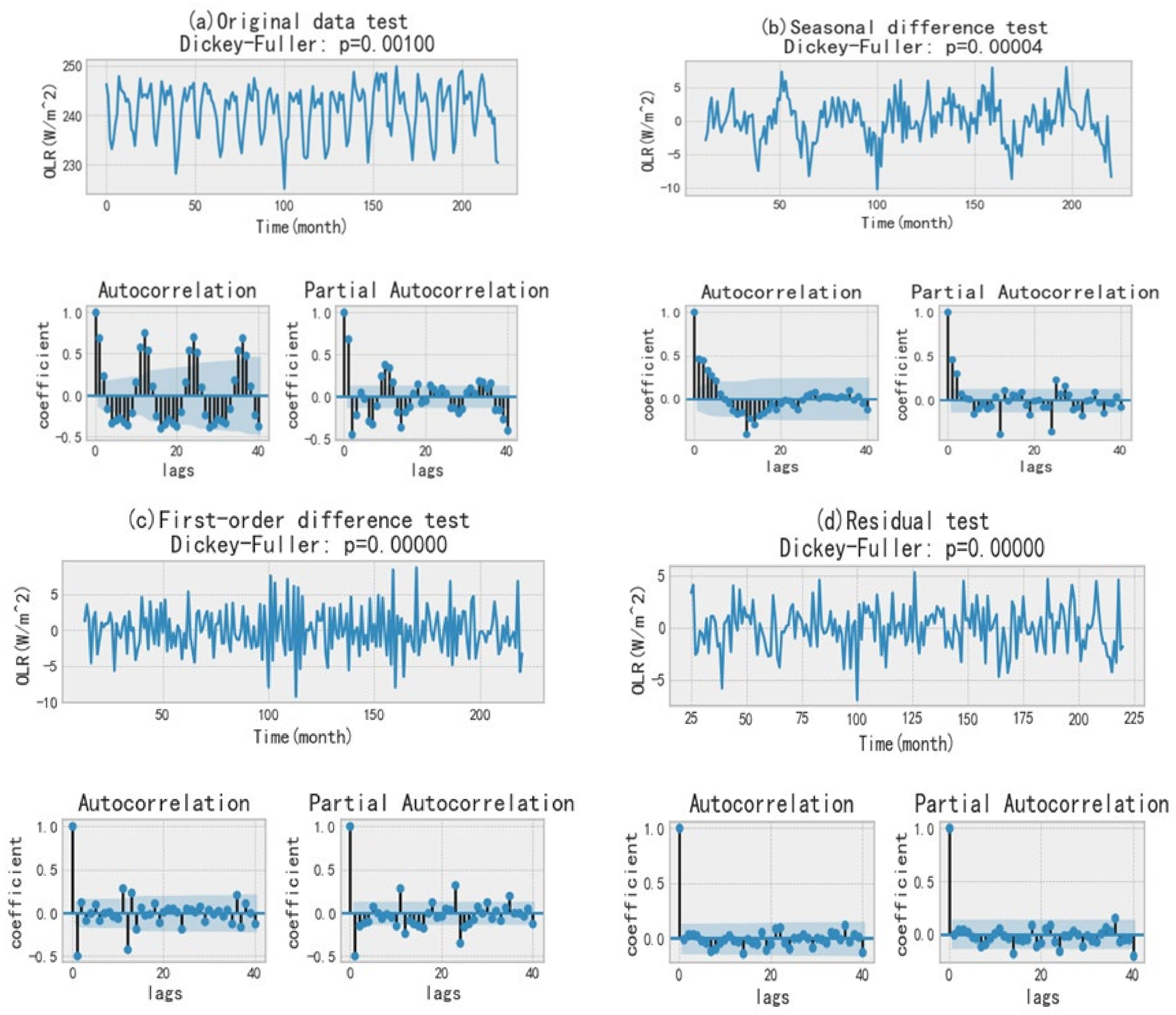
• The time-series data of OLR is plotted;
• The obtained OLR data is plotted to check whether it is a stationary time series; if the result is a non-stationary time series, the obtained OLR data is converted into stationary data through differential processing;
• The autocorrelation coefficient and partial autocorrelation coefficient are calculated for the stable OLR data obtained, and the optimal parameters are obtained through analysis;
• After the above steps, the optimal parameters are obtained by training, and the SARIMA model is established, and then the model is checked for the obtained model, the method for checking its stability is the Dickey–Fuller (DF) test. After the test is stable, the time series changes of the OLR data can be predicted.

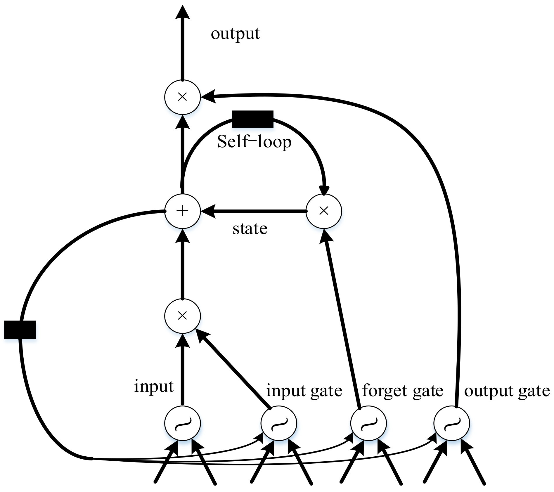
2.2.4. Long Short-Term Memory Algorithm

Long short-term memory (LSTM) algorithm was first proposed by Sepp Hochreiter and Jürgen Schmidhuber in 1997. It is a specific form of recurrent neural network (RNN), and RNN is a general term for a series of neural networks that can process sequence data [20].

The structure of a single node of LSTM is shown in Figure 1 below, which is a threshold RNN. The ingeniousness of LSTM is that, by increasing the input, forgetting and output thresholds [21], the weight of the self-loop is changed, so that when the model parameters are fixed, the integration scale at different times can be continuously changed according to the requirements, thus avoiding the gradient disappearance or the occurrence of swelling problems [22].

According to the structure of the LSTM network, the calculation formula of each LSTM unit is as follows, where $f_t$ represents the forgetting threshold; $i_t$ represents the input threshold; $\widetilde{C_t}$ represents the CELL state at the previous moment, and $C_t$ represents the CELL state (here is where the cycle occurs). $o_t$ represents the output threshold; $h_t$ represents the output of the current unit, and $h_{(t-1)}$ represents the output of the unit at the previous moment.

$$f_t{=\sigma (W}_f{\ast [h}_{t-1}{,x}_t{]+b}_f)$$

(1)

$$i_t{=\sigma (W}_i{\ast [h}_{t-1}{,x}_t{]+b}_i)$$

(2)

$$\widetilde{C_t}{=\mathit{tan}h(W}_C\ast \left[h_{t-1}{,x}_t\right]{+b}_C)$$

(3)

$$C_t{=f}_t\ast C_{t-1}{+i}_t\ast \widetilde{C_t}$$

(4)

$$o_{t }=\sigma \left(W_o\ast \left[h_{t-1}{,x}_t\right]{+b}_o\right)$$

(5)

$$h_t{=o}_t\ast {\mathit{tan}h(C}_t)$$

(6)

3. Inter-Annual Variability Analysis of OLR

3.1. Inter-Annual Variability Trend of Latitude and Longitude OLR

From the inter-annual variability of OLR with latitude in Figure 2a, it can be known that the variation trend of OLR has a zonal distribution characteristic that is symmetrical with the equator. It can be seen from Figure 2a that there are two peaks, and a valley appears in the interval between the two peaks. The OLR value shows an inverted W-shaped change trend. The two peaks appear at about 275 w/m² near the north and south latitudes of 20°, and the valley value appears near the 5° north latitude about 250 w/m². It may be caused by the distribution of clouds. The amount of clouds in the equatorial region shields the long-wave radiation on the surface, and then valleys appear in the equatorial region. The change of OLR value shown in Figure 2a gradually decreases with the increase of latitude, and the minimum value is near the South Pole, which may be related to the long-term low-temperature conditions and the hole in the ozone layer in the Antarctic region. At the same time, we can find that the change characteristics of OLR values in low latitudes are not particularly obvious, while the changes in OLR values in middle and high latitudes are relatively significant. As can be seen from Figure 2b, the longitude change of OLR presents a W-shaped change trend as a whole, and it has a very low valley value of 216 w/m². In the vicinity of about 95° east longitude, after consulting relevant information, this extremely low valley value may be caused by the surface temperature of the Qinghai-Tibet Plateau, the third pole of the earth. Although the trend of longitude is W-shaped, it is still quite different from the variation range of latitude OLR. The latitude OLR value varies within the range of 140 w/m²~280 w/m², and the range of variation is larger. The longitude OLR value varies in the range of 215 w/m²~235 w/m², and the variation range is small.

3.2. Annual Average OLR Change and MK Analysis in China

Figure 3a is obtained by averaging the OLR data detected by AIRS from 2003 to 2020. From Figure 3a, it can be seen that the OLR value showed a downward trend from 2003 to 2012 and reached the lowest value in 2012. After 2012, it showed an upward trend and reached its highest value in 2015. At the same time, MK analysis is performed on the processed annual average OLR data. As shown in Figure 3b, the intersection (mutation point) of UF (forward sequence curve) and UB (reverse sequence curve) are in the range of $U_{0.05}=\pm 1.96$; it met the 95% confidence level and has reference significance. Its mutation point is after 2015, and all of them are a negative value, indicating that the OLR value detected by AIRS has decreased since 2015.

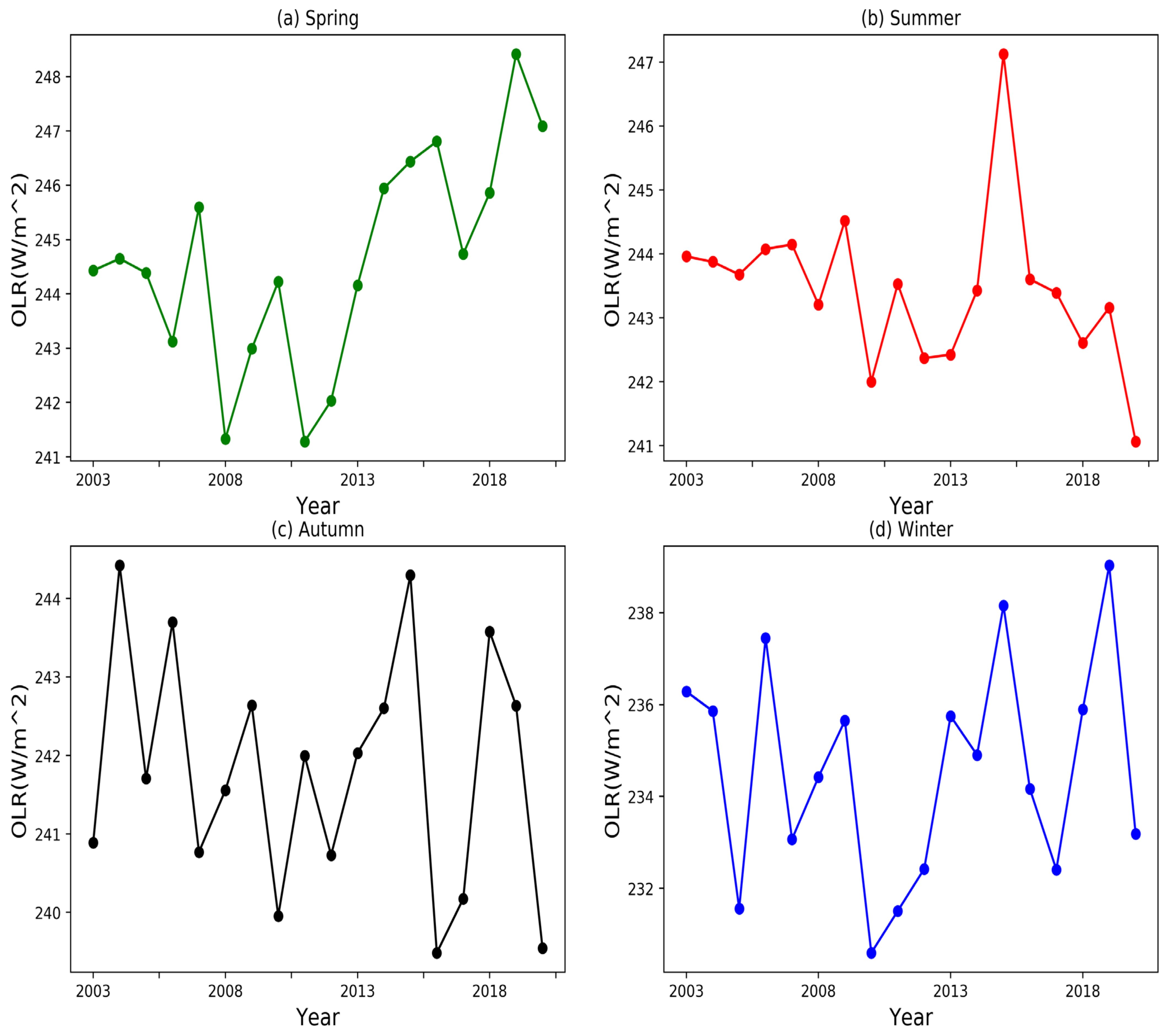
3.3. Inter-Annual Variability Trend of OLR in Different Seasons in China

Figure 4 shows the change trend of OLR in each season in China. On the whole, it can be seen that the value of OLR in spring, summer and autumn is higher than that in winter. From Figure 4a, the OLR value in spring as a whole shows a V-shape, with a downward trend from 2003 to 2011. After 2011, the OLR value in spring showed an upward trend and reached the maximum value in 2019 with a value of 246 w/m². As shown in Figure 4b, the summer OLR value increased from 2003 to 2007, showed a downward trend from 2007 to 2012, gradually increased after 2012 and decreased after 2015, showing a downward trend as a whole, reaching the maximum value in 2015. The value of OLR was about 249 w/m². From Figure 4c, the OLR value in autumn showed a downward trend from 2004 to 2010. After 2010, it gradually increased and reached the maximum in 2015 and then showed a downward trend. As shown in Figure 4d, the winter OLR value showed a W-shaped change trend from 2003 to 2015 and a V-shaped change after 2015, with low values in 2005, 2010 and 2017 and high values in 2006 and 2015.

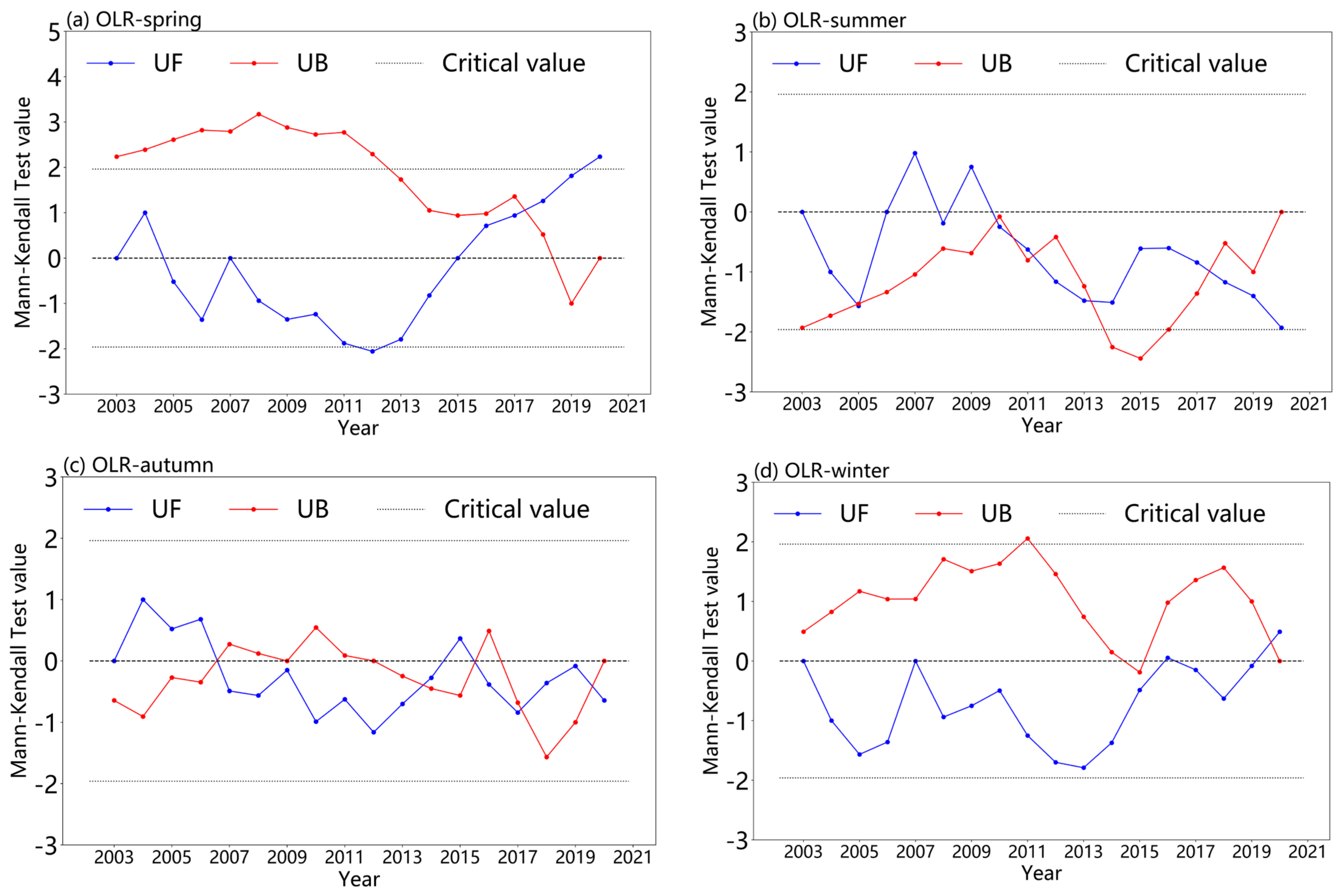
3.4. MK Seasonal Analysis of OLR in China

MK mutation analysis was performed on the OLR data detected by AIRS from 2003 to 2020 (as shown in Figure 5). It can be seen that there will be one or more intersections of MK changes in the four seasons during the 18 years, and the seasonal mutation points with mutation points are all within the range of $U_{0.05} =\pm 1.96$. As shown in Figure 5a, the spring mutation occurred in 2017, and the mutation point was positive, indicating that OLR was an increasing trend after 2017. From Figure 5b, the summer mutation point is around 2011, but its mutation points are all negative values, indicating that the change of OLR change in 2011 is decreasing. Similarly, as shown in Figure 5c, we can know that there are many intersection points in autumn and that all of them are negative, but we cannot judge the position of the mutation point, only that it shows a downward trend. From Figure 5d, the winter node is before 2020, so no mutation occurs.

4. Spatial Characteristic Analysis of Outgoing Longwave Radiation (OLR)

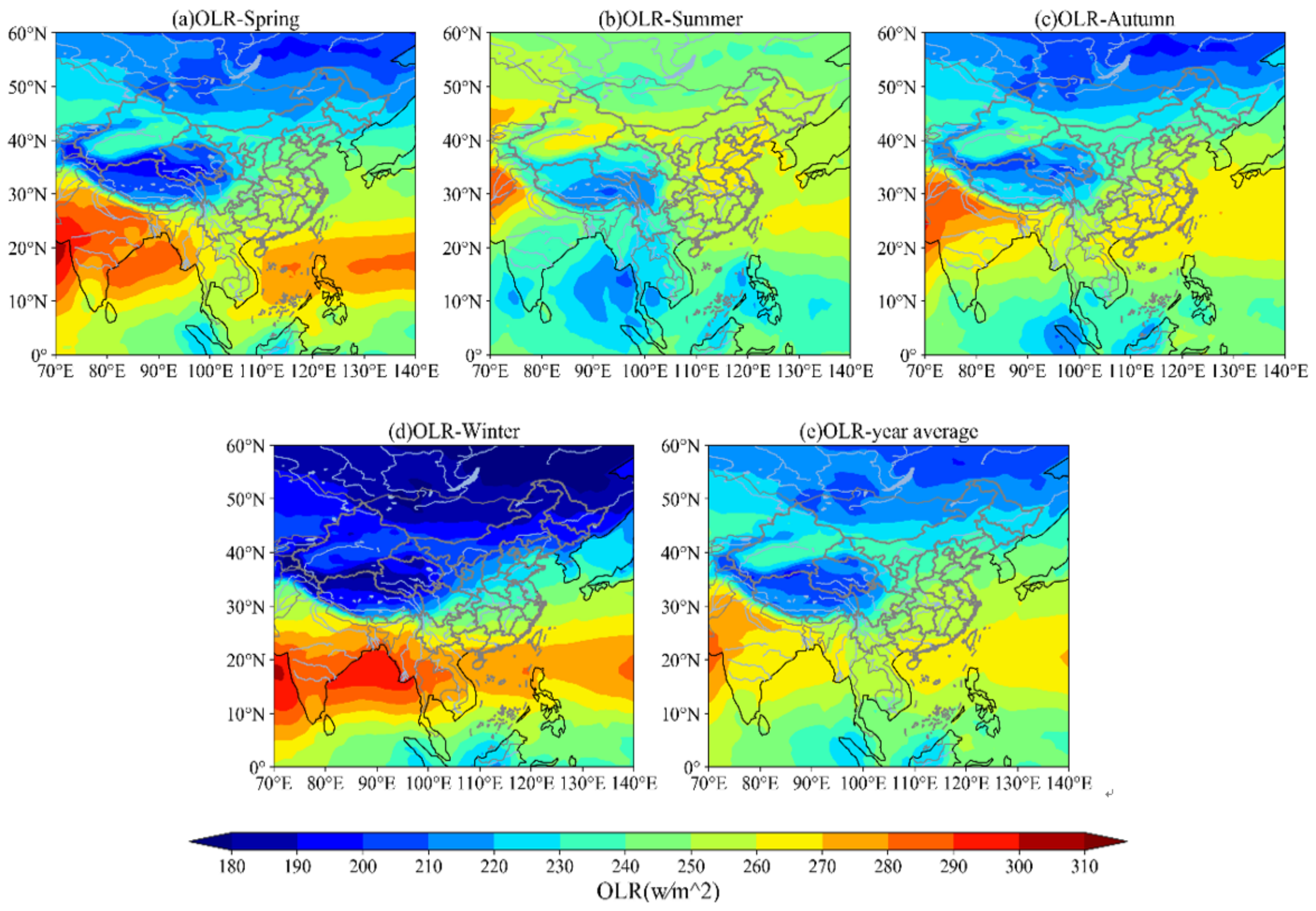
4.1. Spatial Characteristic Distribution of Four-Season and Multi-Year Average OLR in China

Figure 6 shows the distribution of the spatial characteristics of the four-season and multi-year average OLR in China from 2002 to 2021. From the five pictures in Figure 6, it can be seen that the spatial distribution of features is zonal as a whole, because the lower the latitude, the higher the ground temperature and the greater the OLR. On the contrary, the higher the latitude, the lower the ground temperature and the OLR. So the region of China above 40° north latitude presents a low-value area, and the region of China below 40° north latitude presents a high-value area. At the same time, we can find that the OLR value in the Qinghai-Tibet Plateau region is significantly lower than other regions at any time. This may be due to the higher altitude in the Qinghai-Tibet Plateau region and the lower surface temperature, so the OLR value is always lower at any time period in the Qinghai-Tibet Plateau region. It can be seen from Figure 6 that the OLR values in spring and winter are lower than those in summer and autumn, which may be caused by the temperature of the underlying surface and cloud conditions. According to the overall display in Figure 6, we can clearly see that the north–south boundary in China is divided into high-value areas and low-value areas, which have a certain relationship with the north–south boundary. The high-value areas are mainly in Hainan Island. It may be because Hainan has a tropical monsoon climate, with summer and without cold winter all year round and with sufficient sunlight and strong light potential, so the OLR value in this region is higher than other places. The low-value area in the north has obvious low-value areas, such as the northeast region and the Qinghai-Tibet Plateau; mainly the northeast region has a temperate monsoon climate. Due to the high latitude, it is close to the birthplace of the winter monsoon in northern Asia, and the duration of the cold in winter is longer. At the same time, the rainfall here is concentrated in summer, and snowfall more and lasts for a long time in winter. It is also affected by the cold pole of the northern hemisphere, which leads to a relatively obvious low-value area of OLR. The Qinghai-Tibet Plateau region is mainly due to its higher altitude and less cloud cover, resulting in less sunlight and lower surface temperature, which eventually leads to a significantly lower OLR area. Locally, we can find that winter is the lowest among the four seasons, and summer is the highest among the four seasons, which can well correspond to the inter-annual variability. This shows that the spatial characteristic distribution of OLR has a good corresponding relationship with latitude, cloud, precipitation, temperature and other data.

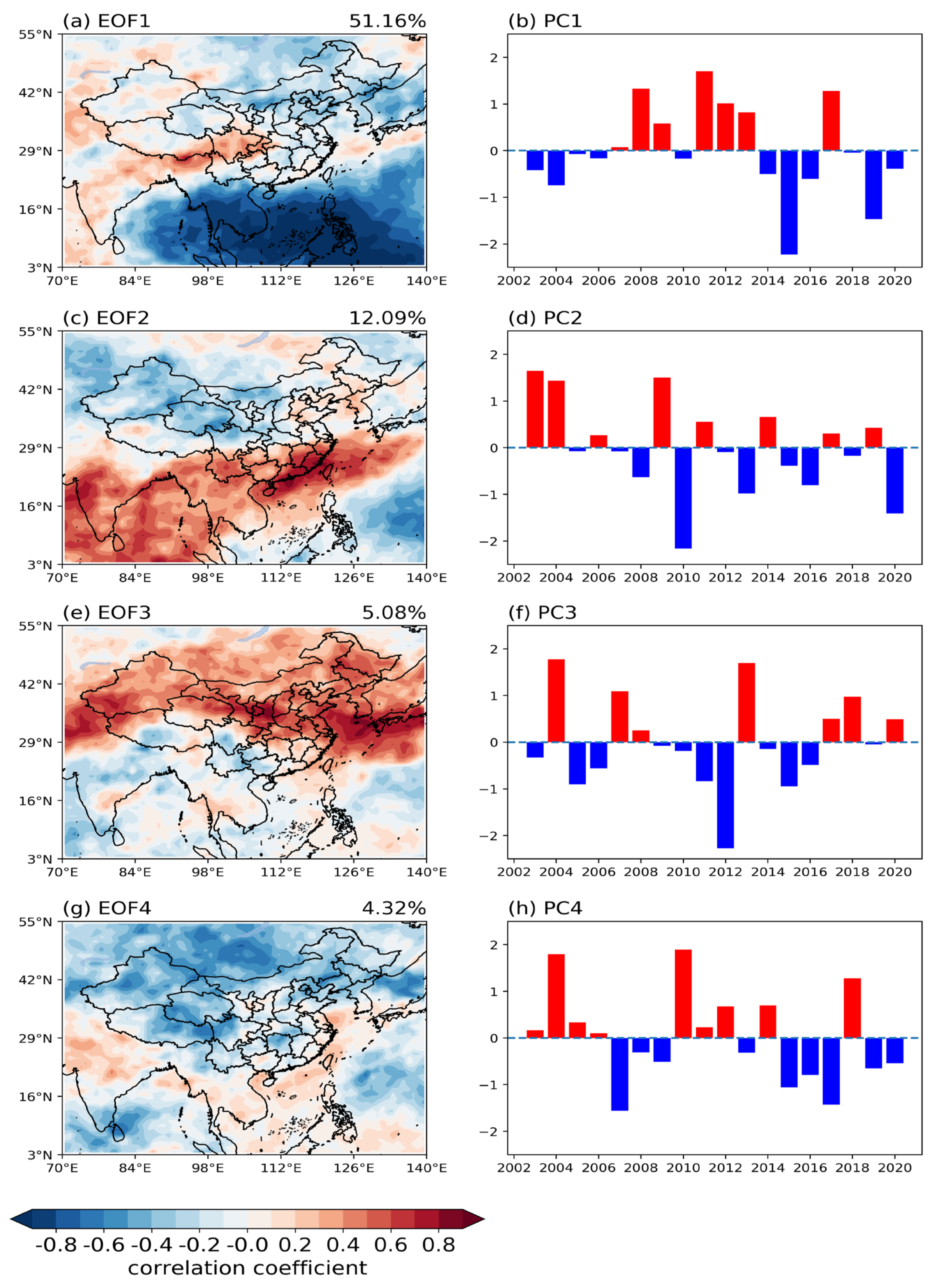
4.2. The Annual Average Spatiotemporal Characteristic EOF of OLR in China

Anomaly processing was performed on the OLR data detected by AIRS during the 18 years from 2003 to 2020 to obtain the annual average anomaly field data. Then, the anomalous field data were decomposed by EOF to obtain the eigenvectors and time coefficients. From a physical point of view, the larger the variance contribution of the eigenvectors obtained by the decomposition, the more it can reflect the spatial variation characteristics of the OLR data inverted by AIRS. At the same time, the time coefficient is used as the weight of the eigenvectors, which can reflect the spatial contribution influence of different years to spatial features.

Using EOF decomposition, we obtained 4 eigenvectors and 4 time coefficients, and the variance contribution and cumulative variance contribution of the eigenvectors are as follows (

Table 1. The variance contribution and cumulative variance (unit: %) of the first 4 modes.

Mode	EOF1	EOF2	EOF3	EOF4
Variance contribution	51.16%	12.09%	5.08%	4.32%
Cumulative variance	51.16%	63.25%	68.33%	72.65%

):

According to Table 1, it is known that the total variance contribution exceeds 70%, which is significant. It can be seen from Figure 7a that the variance contribution of the first EOF1 is 51.16%, far exceeding other modes. Its spatial distribution presents a meridional structure of ‘+, −’; 70°~110° E is positive, and 110°~140° E is negative. From Figure 7b, it can be seen that the time coefficient PC1 shows that the negative value is 11 years, and the positive value is 7 years, indicating that the change in OLR value in the whole 18 years showed a downward trend. But it showed an upward trend before 2013 and showed a significant downward trend after 2013. As shown in Figure 7c, the contribution of the second mode variance of the EOF2 is 12.09%, and it can be seen that the ‘+, −’ changes are divided by the north–south dividing line in China. The south of the dividing line is positive, and the north is negative. Guangdong and Fujian regions showed positive values, and the Qinghai-Tibet Plateau region showed more obvious negative values. From Figure 7d, it can be known from PC2 that the positive value is 8 years, and the negative value is 10 years. After 2009, the overall trend showed a downward trend, and the time coefficient was the lowest in 2010, indicating that the OLR inversion by AIRS in 2010 declined more sharply. As shown in Figure 7e, the variance contribution of the third mode of EOF3 is 5.08%, which can be clearly seen to be a zonal distribution; 30°~55° is a ‘+’ value, and below 30° is a ‘−’ value. From Figure 7f of the PC3 time coefficient, it can be seen that the overall trend is first rising and then falling, and it was rising before 2009, and the most obvious decline in 2012. As show in Figure 7g, the variance contribution of the fourth mode of EOF4 is 4.32%. This variance contribution is small and has no reference value in theory. It can also be seen from EOF4 that it is basically a negative trend in the entire Chinese region. It means that this variance contribution has no reference significance. As show in Figure 7h, it can be seen from the PC4 time coefficient that the positive value is 9 years and that the negative value is 9 years, indicating that the OLR value has not changed as a whole during these 18 years. This also shows that this variance contribution has no reference value.

5. Prediction Model Construction and Result Analysis

5.1. Predictive Analysis of SARIMA

5.1.1. Stationarity Test

Figure 8a is the initial sequence test of the outgoing long-wave radiation. We set the lag of the autocorrelation coefficient in Figure 8a to 40. From Figure 8a, it can be seen that the range changes of the OLR data is 230–250 w/m², and it can be seen that the initial time series of OLR data is stationary. Since the initial series of OLR data is stationary, the Dickey–Fuller (DF) test rejects the null hypothesis of the existence of a unit root. In fact, this can also be seen from the graph of Figure 8a itself—there is no obvious trend, so the mean is constant, and the variance of the whole series is relatively stable, so we only need to deal with seasonality. When we use “seasonal difference” for the time series of OLR data, that is perform a simple subtraction operation on the series, the time difference is equal to the seasonal period (here we set the seasonal period to 12, because a year is 12 months), obtained through an experimental seasonal-difference test plot (Figure 8b). By observation, the p-value in DF dropped from 0.00100 to 0.00004, indicating the disappearance of seasonality in the graph. It can be seen from the autocorrelation function (ACF) in Figure 8b that its periodicity disappears, and it can also be clearly seen that the seasonality disappears. Later, we also found that there are more points outside the light shade from the ACF in Figure 8b, which shows that the time series of OLR data still has too many obvious lags, so in order to move to divide them, we will “first-difference” (subtract itself from the series (with a time difference of 1) of the OLR data time series), and then we get the first-order difference test plot Figure 8c. From Figure 8b to Figure 8c, we can see that the time series of OLR data varies from −10–10 to −5–5, and it is found that the time series of OLR data oscillates around zero, and from the disordered oscillation in Figure 8b to the stable oscillation change in Figure 8c, the DF test shows that it is stable, and we can also find that the ACF is shallow in the number of points in the shaded area being significantly reduced, indicating that the time-series lag of the OLR data is significantly reduced, and it can be seen that the significant spikes in the ACF disappear. After using residual analysis, we get Figure 8d. At this time, we can predict the OLR time series data.

5.1.2. Other Results Estimating Parameter Performance

It can be seen from Figure 9 that the prediction results of the OLR data have very good performance results, because it can be seen from the standardized residual diagram. The variation ranges of the standardized residual of the OLR data obtained by the standardized residual processing is within the range of −2–2, and it oscillates around zero, indicating that its effect is better. At the same time, we can see from the histogram plus estimated density that the change of the histogram is mainly concentrated around zero, which is consistent with the change range of the standardized residual, indicating that the change of the standardized residual of the OLR data between −2–2 is correct. It can also be seen from the distribution of the normal distribution and the kernel density estimation (KDE) that the sum of their areas of change is 1, which basically conforms to the function change of the normal distribution, indicating that the effect of SARIMA prediction is good and that it is worthy of reference. After that, we correlate the quantiles of the samples and the quantiles of the theoretical, and we can find that their changes are on a linear line, indicating that their correlation is very high, and the reference of the prediction results that can obtain the OLR data should be high. Finally, we analyze the correlation diagram of the data, and we can find that the range of the correlation points is basically within the light-shaded area, indicating that there is basically no lag process in the change of OLR data, indicating that the prediction results are better. In summary, it can be found that the prediction of OLR data with the SARIMA algorithm should be of great reference value.

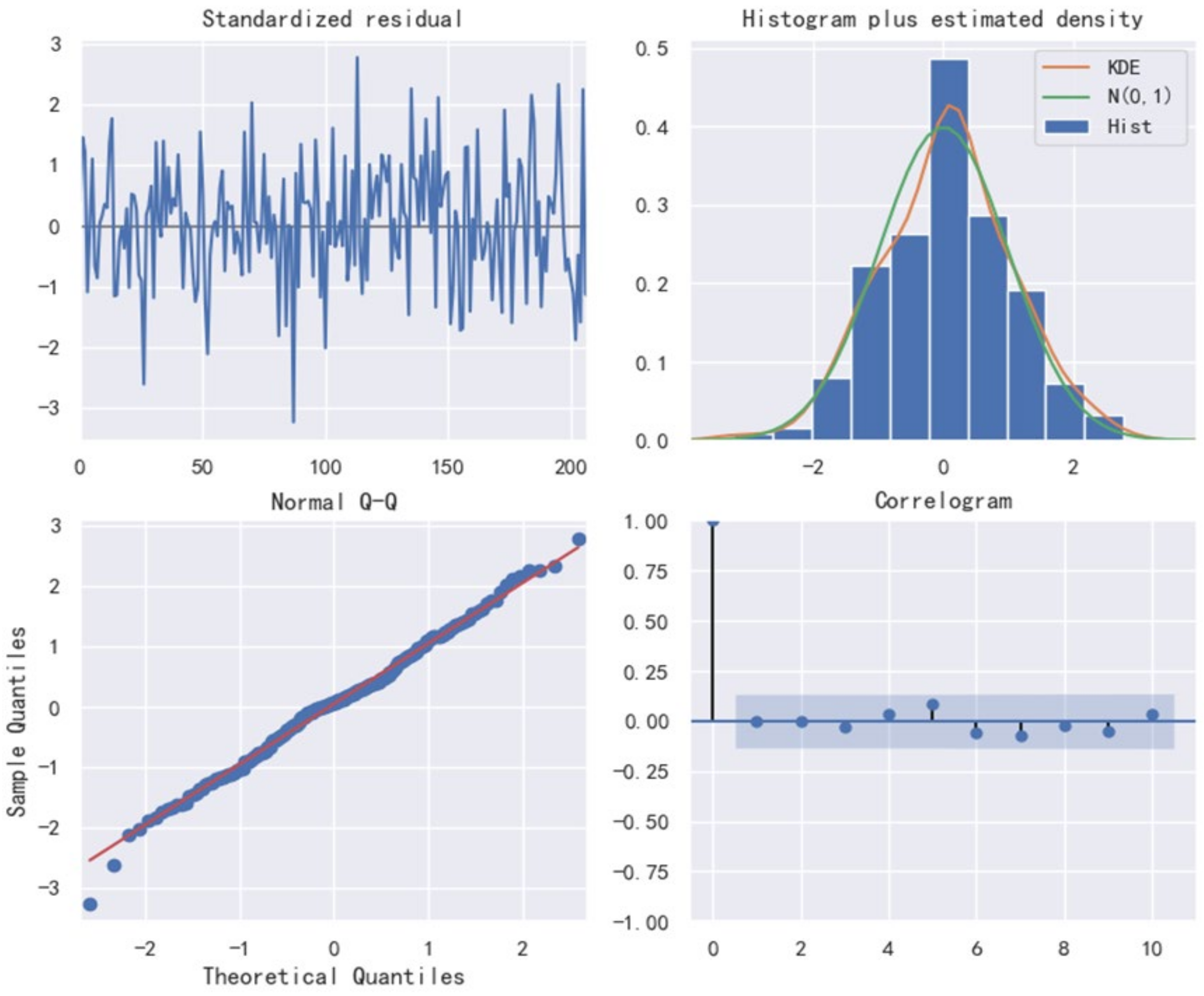
5.1.3. Modeling, Diagnosis and Prediction

Modeling SARIMA (seasonal autoregressive moving average model) requires the selection of some parameters. The optimal parameter value SARIMAX (1,1,3) × (1,1,1,12) is finally obtained through parameter training.

After the model is built, it is necessary to test its residuals. It is mainly necessary to ensure that the residuals of our model are irrelevant. By drawing the residual distribution of the model as shown in Figure 8d, confirming the low correlation between time-series residual and its own lag version by residual autocorrelation. It can be seen that our model produces a satisfactory fit that can help us better understand time series data and predict future values. Finally, the trend of OLR in the next 36 months is obtained through this model, as shown in Figure 10. The abscissa represents the month, and the ordinate represents the values of OLR. It was found that the OLR value showed a decreasing trend, and the error under the condition of percentage error is 0.01%, and the accuracy is very high. It is indicating that the accuracy under the condition of percentage error is extremely high, which can reach close to 99%. It is of great reference value to study the effects of OLR on cloud cover, sea surface temperature and precipitation.

5.2. Model Construction and Predictive Analysis of LSTM Predictive Analysis

First, the original data is processed, the data characteristics of the time series data of OLR in China is normalied and the data is mapped to the interval [0,1]; convert the time-series problem is converted into a supervised learning problem through a sliding window; then the dataset is divided into two parts: the training set and the test set. According to the LSTM network input format requirements, the numpy.reshape function is used to perform matrix transformation, so that the format is 3-dimensional data input into the model. The structure of the model is shown in

Table 2. LSTM network structure table.

Layer (Type)	Output Shape	Param
Lstm_1 (LSTM)	(None, None, 50)	10400
Lstm_2 (LSTM)	(None, None, 100)	60400
Lstm_3 (LSTM)	(None, None, 200)	240800
Lstm_4 (LSTM)	(None, 300)	601200
Dropout (Dropout)	(None, 300)	0
dense_1 (Dense)	(None, 100)	30100
dense_2 (Dense)	(None, 1)	101
activation (activation)	(None, 1)	0

.

The number of training epochs is set to 100, and the error changes during the training process of the LSTM model are shown in Figure 11.

When the number of epochs of this training is set to 100, the results of the training error of the LSTM model are shown in Figure 11. From Figure 11, we can see that, when our training continues after 60 epochs, the error basically tends to stability. Furthermore, we can see that, after 60 epochs of training, the loss of error is below 0.05, close to about 0.03, indicating that the accuracy of the model is close to 97% and that the accuracy is already very high and also indicating its very high reference significance. The actual value of OLR and the predicted value of LSTM neural network are shown in Figure 12. The best first-order root mean square error RMSE for the test set and training set is 4.05 and 4.04, respectively. It can be seen that the prediction effect of the LSTM neural network model is good. Using the existing OLR data to predict the OLR in the next month has achieved the expected results. The predicted value of 233.2 w/m² can better fit the real value, so that the error is relatively small and has a relatively high reference value.

6. Discussion and Conclusions

6.1. Discussion

This paper uses the nearly 19 years of OLR data in AIRS from September 2002 to February 2021 to analyze its spatiotemporal, seasonal, modes and forecast results. First of all, through the analysis of spatiotemporal and seasonal results, we can know the year-to-year changes and spatial distribution in China. Through the changes of OLR, we can better study some weather, such as precipitation, sea temperature, cloud cover, etc. to provide some help. In past research, there has been little direct study of OLR data, so our research idea is relatively new among the authors of OLR data research.

Among some outstanding authors in the world recently, the research on OLR mostly focuses on the study of OLR anomalies before and after earthquakes, and the method of useful background field analysis focuses on the increment of the multi-year average value of OLR data [23]. Some researchers studied whether the OLR data is abnormal before the earthquake nucleation in the seismically active area to determine whether the earthquake is nucleated [24], and some researchers study whether the OLR data will have an impact on the ionosphere disturbance before the earthquake and the correlation with some parameter changes, etc. [25]. Most of the studies are done in the context of earthquakes. However, this paper directly studies the OLR data and finds that the change of the OLR data is seasonal, and the overall change trend of the OLR decreases with the increase of latitude. At the same time, mutation analysis was performed on OLR data to study whether there were abnormalities in OLR data in the past 19 years, and the reasons for the formation of these abnormal points. This is relatively rare in previous studies, and the ideas are relatively new.

In the research process of this paper, we conducted an EOF analysis on the annual average OLR data, and it can be found that the total contribution of the four modes after EOF decomposition is more than 70%. In the process of data analysis by existing researchers using the EOF method, the variance contribution of the first mode is often relatively large, for example in Hu’s study of winter precipitation in California [26] and Wie’s study of surface ozone changes [27]. The first mode of its EOF is higher than 70%, indicating that its first mode has a high reference value. The total contribution of our modes is higher than 70%, but the variance contribution of the first mode exceeds 50%, and the other modes are relatively small, which may be caused by the complicated changes in OLR. However, we can still find abnormal changes in the Qinghai-Tibet Plateau and Northeast China, which are caused by the topography of the Qinghai-Tibet Plateau and the climatic environment in Northeast China.

Finally, we conduct predictive research on OLR data, which is relatively rare among researchers of OLR data over the years, and OLR data has a relatively prominent research significance. At the same time, the percentage errors of the two algorithms in the prediction results are relatively high, which is of high reference significance. However, the change of OLR is relatively complicated, and a single prediction is definitely not enough. Because the change of OLR will be affected by some extreme weather, we need to do more in-depth research in the future.

6.2. Conclusions

Using SARIMA and LSTM methods to study the characteristic distribution and prediction results of the China regional OLR value, the following conclusions are summarized:

(1)

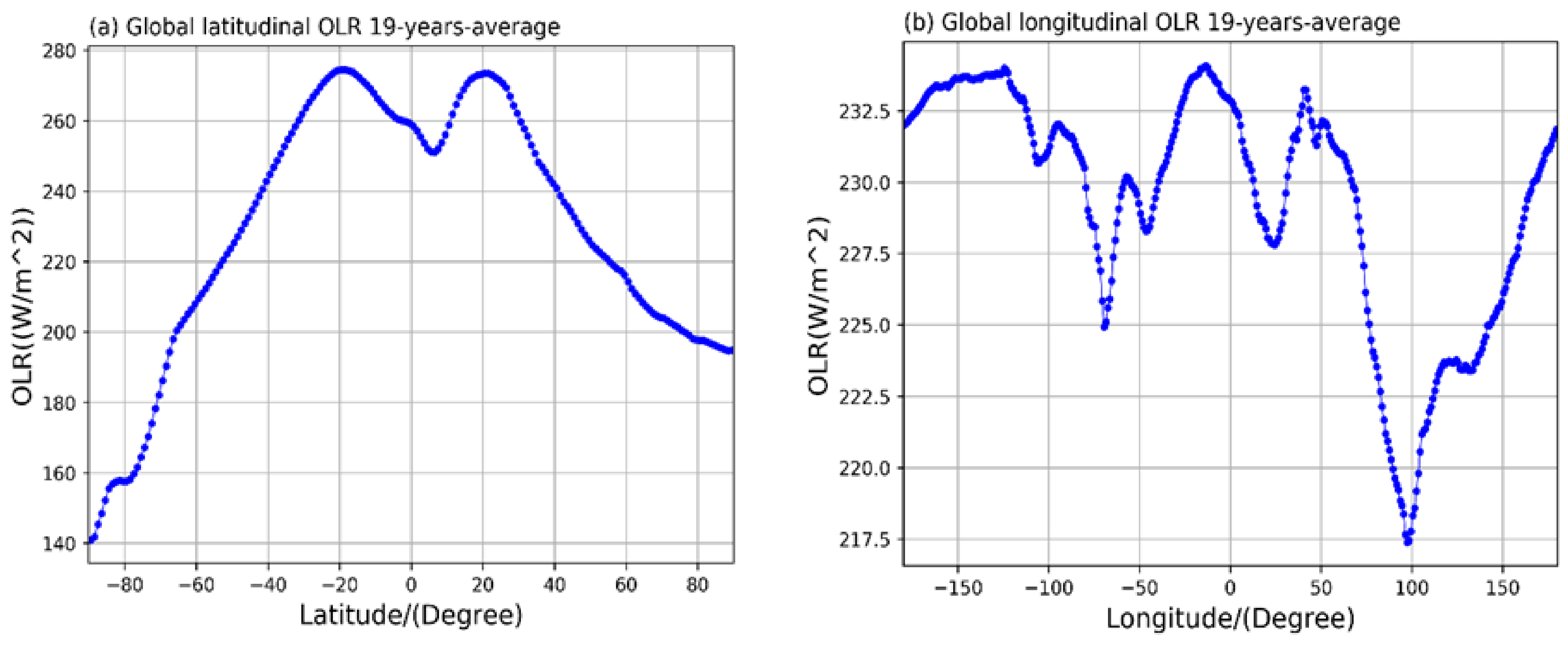
The distribution of OLR detected by AIRS presents a zonal distribution characteristic that is symmetrical to the equator, and the OLR gradually decreases with the increase of latitude. Low latitudes have no obvious change characteristics, while middle and high latitudes have more obvious changes. Furthermore, the change of latitude shows an inverted W-shaped change trend, and the change of longitude shows a W-shaped change trend.

(2)

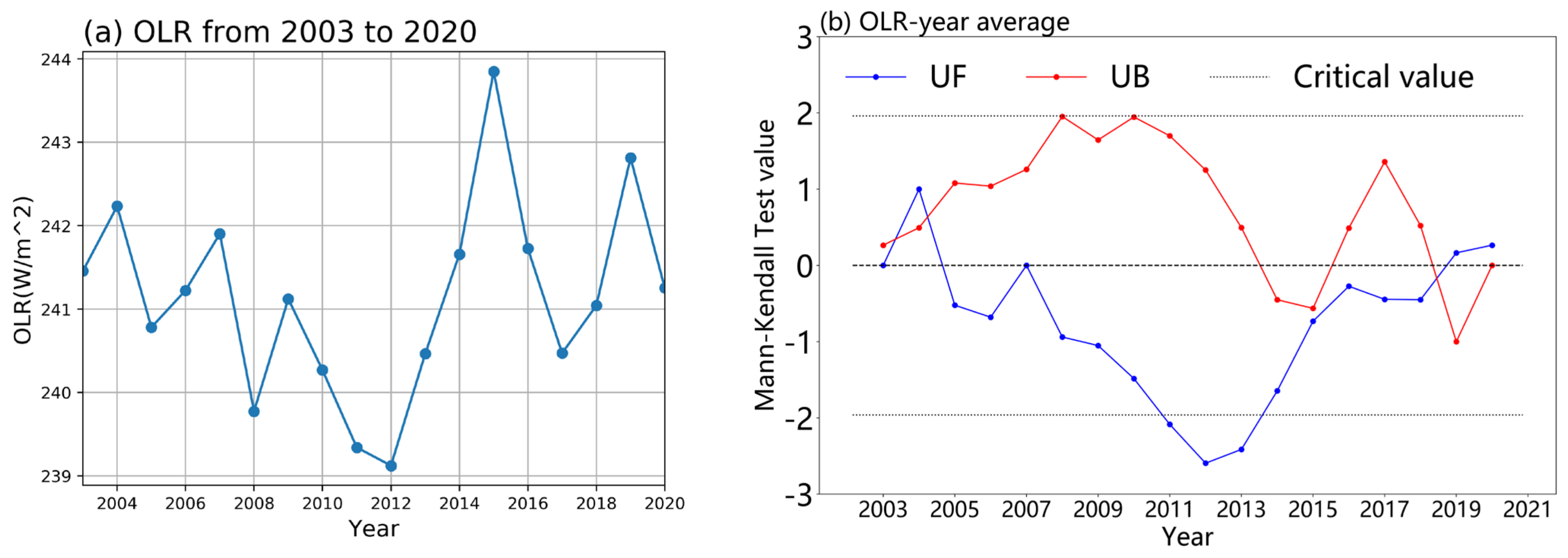
The annual average change of OLR value detected by AIRS was the largest in 2015 and the smallest in 2012. The annual average OLR MK analysis showed a downward trend in OLR values after 2015. The OLR value of the four seasons changes in spring, summer and autumn is obviously higher than that in winter, and the winter in 2010 is the lowest value among the four seasons. Four seasons of MK analysis shows that there are mutation points in spring, summer and autumn but no mutation points in winter, as well as a sudden change to increasing in spring and a trend of decreasing in summer and autumn.

(3)

The spatial distribution of OLR values detected by AIRS varies with latitude. The higher the latitude, the smaller the value. Furthermore, the annual average change high- and low-value area is divided by the north–south dividing line in China, the OLR value of the four seasons is significantly lower in winter than in other seasons, and the change is more obvious in Qinghai-Tibet Plateau and Northeast China.

(4)

By decomposing EOF into four spatial features and four time coefficients, it can be seen that its total variance contribution exceeds 70%, and the variance contribution of the first mode exceeds 50%, which is much higher than that of other modes. The spatial features and the time coefficient shows that the changes in the Qinghai-Tibet Plateau and Northeast China are more obvious.

(5)

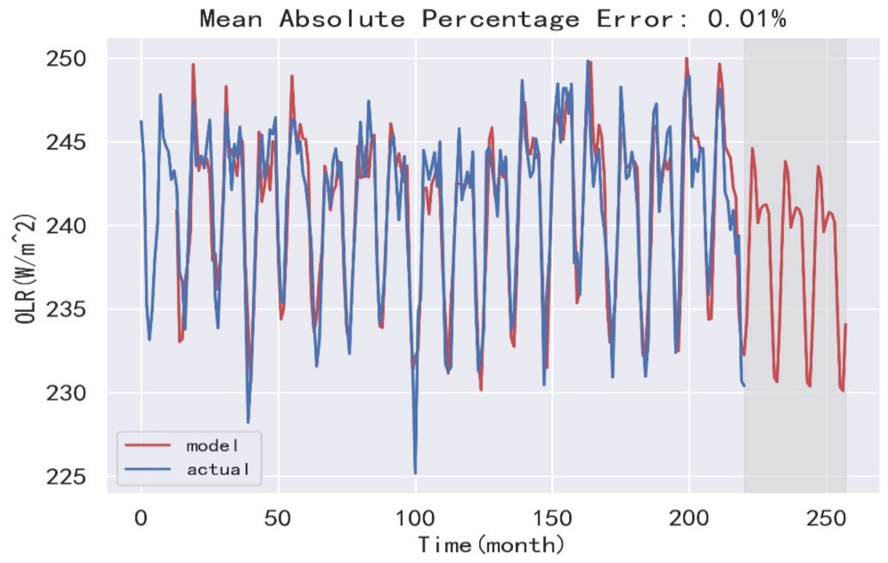
Prediction analysis through SARIMA algorithm can predict the OLR data for the next 36 months. It can be seen that the percentage of error in the prediction result is only 0.01%, that the accuracy is very high, and that the future OLR value in the prediction result has a slight downward trend. It can provide some reference value for future research on extreme weather.

(6)

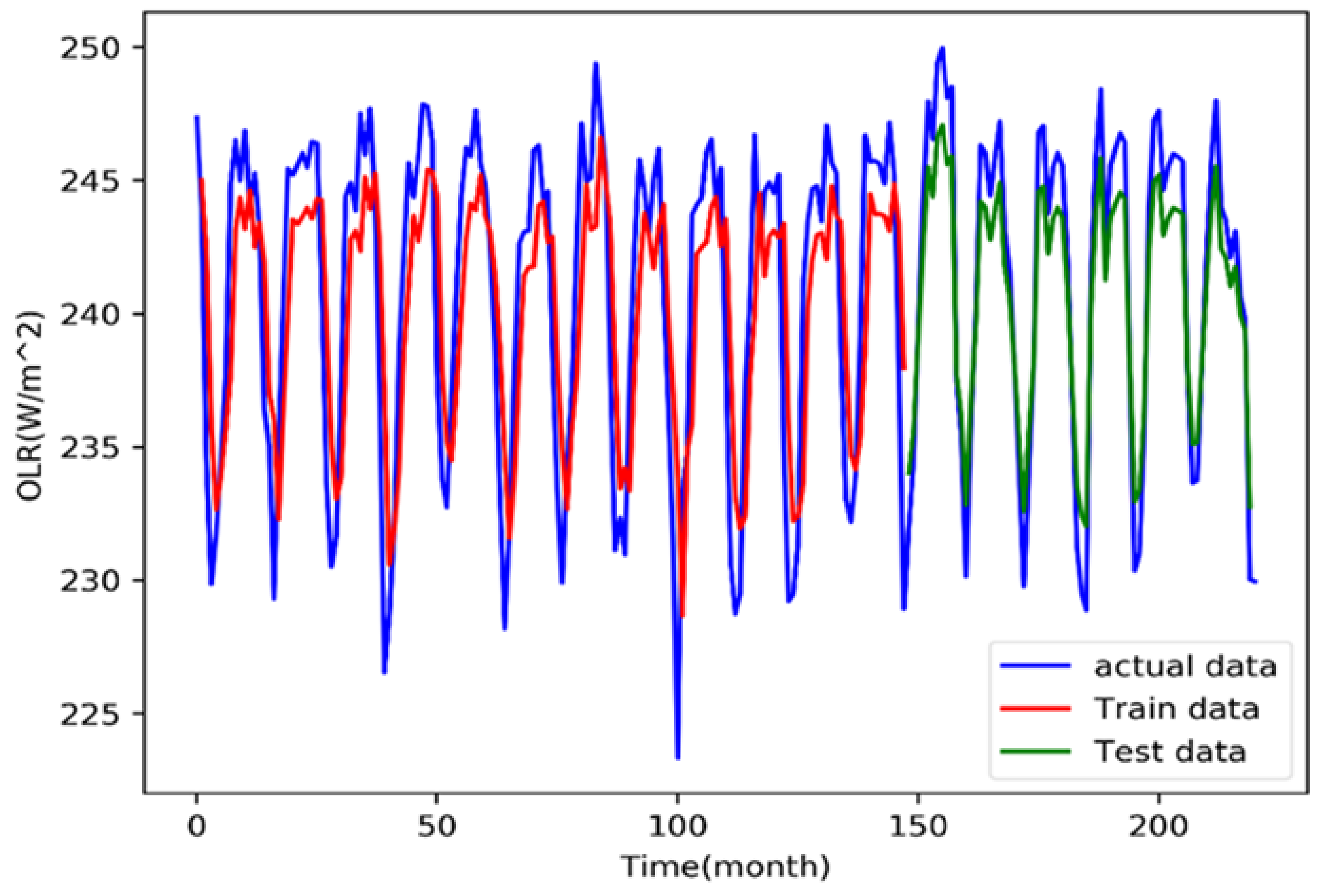
The prediction of the LSTM algorithm can be obtained after 60 instances of training; its loss degree is about 0.03, and the obtained accuracy is about 97%, which is very satisfactory for the reference value. However, compared with the SARIMA algorithm, the accuracy is slightly lower. It shows that SARIMA algorithm has a better prediction effect than LSTM algorithm.

Although this paper analyzes the change of OLR value in China through the temporal and spatial distribution of the four seasons and uses two algorithms for prediction and analysis, the change of OLR will be affected by some extreme weather, such as cloudiness, precipitation, and the temperature of the underlying surface. Therefore, the change process of OLR is quite complicated. This article only predicts the existing data without considering some factors affecting extreme weather. Therefore, to find out its growth and decline trends, it is necessary to use more detailed data and methods to analyze and demonstrate.

References

1. Xin, W.; Congming, D.; Pengfei, W.; Chaoli, T.; Fengmei, Z.; Heli, W. Information analysis of airborne atmosphere infrared high resolution spectral. Infrared Laser Eng. 2019, 48, 1104004. [Google Scholar]
2. Sandeep, S.; Stordal, F. Use of daily outgoing longwave radiation (OLR) data in detecting precipitation extremes in the tropics. Remote Sens. Lett. 2013, 4, 570–578. [Google Scholar] [CrossRef]
3. Nalli, N.R. Validation of Near-Real-Time NOAA-20 CrIS Outgoing Longwave Radiation with Multi-Satellite Datasets on Broad Timescales. Remote Sens. 2021, 13, 3912. [Google Scholar]
4. Lee, H.T.; Gruber, A.; Ellingson, R.G.; Laszlo, I. Development of the HIRS Outgoing Longwave Radiation Climate Dataset. J. Atmos. Ocean. Technol. 2007, 24, 2029–2047. [Google Scholar] [CrossRef] [Green Version]
5. Liu, L.; Zhang, W.; Chen, W.; Wu, R.; Wang, L. Evaluation of FY-3B Reprocessed OLR Data in the Asian–Australian Monsoon Region during 2011–2019: Comparison with NOAA OLR. J. Meteorol. Res. 2021, 35, 964. [Google Scholar] [CrossRef]
6. Schreck, C.; Lee, H.T.; Knapp, K. HIRS Outgoing Longwave Radiation—Daily Climate Data Record: Application toward Identifying Tropical Subseasonal Variability. Remote Sens. 2018, 10, 1325. [Google Scholar] [CrossRef] [Green Version]
7. Pagano, T.S.; Aumann, H.H.; Broberg, S.E.; Cañas, C.; Manning, E.M.; Overoye, K.O.; Wilson, R.C. SI-Traceability and Measurement Uncertainty of the Atmospheric Infrared Sounder Version 5 Level 1B Radiances. Remote Sens. 2020, 12, 1338. [Google Scholar] [CrossRef] [Green Version]
8. Mariano, A.; Carolina, V.; George, K. MJO Modulating the Activity of the Leading Mode of Intraseasonal Variability in South America. Atmosphere 2017, 8, 232. [Google Scholar]
9. Herdies, D.L. Dynamic Characteristics of the Circulation and Diurnal Spatial Cycle of Outgoing Longwave Radiation in the Different Phases of the Madden–Julian Oscillation during the Formation of the South Atlantic Convergence Zone. Atmosphere 2021, 12, 1399. [Google Scholar]
10. Kim, B.Y.; Lee, K.T. Using the Himawari-8 AHI Multi-Channel to Improve the Calculation Accuracy of Outgoing Longwave Radiation at the Top of the Atmosphere. Remote Sens. 2019, 11, 589. [Google Scholar] [CrossRef] [Green Version]
11. Heli, W.; Congming, D.; Chaoli, T.; Pengfei, W.; Honghua, H.; Xuebin, L.; Wenyue, Z.; Ruizhong, R.; Yingjian, W. Atmospheric parameter model and its application in calculation of radiative atmospheric transport. Infrared Laser Eng. 2019, 48, 11–18. [Google Scholar]
12. Fajary, F.R.; Hadi, T.W.; Yoden, S. Contributing Factors to Spatiotemporal Variations of Outgoing Longwave Radiation (OLR) in the Tropics. J. Clim. 2019, 32, 4621–4640. [Google Scholar] [CrossRef]
13. Zhang, L.; Ding, M.H.; Bian, L.G. AIRS temperature and ozone profiles in the South Pole. Chin. J. Geophys. 2020, 63, 1318–1331. [Google Scholar]
14. Heng, Z.; Jiang, X. An Assessment of the Temperature and Humidity of Atmospheric Infrared Sounder (AIRS) v6 Profiles Using Radiosonde Data in the Lee of the Tibetan Plateau. Atmosphere 2019, 10, 394. [Google Scholar] [CrossRef] [Green Version]
15. Liu, J.; Hagan, D.; Liu, Y. Global Land Surface Temperature Change (2003–2017) and Its Relationship with Climate Drivers: AIRS, MODIS, and ERA5-Land Based Analysis. Remote Sens. 2020, 13, 44. [Google Scholar] [CrossRef]
16. Sun, J.; McColl, K.A.; Wang, Y.; Rigden, A.J.; Lu, H.; Yang, K.; Li, Y.; Santanello, J.A., Jr. Global evaluation of terrestrial near-surface air temperature and specific humidity retrievals from the Atmospheric Infrared Sounder (AIRS). Remote Sens. Environ. 2021, 252, 112146. [Google Scholar] [CrossRef]
17. Amiri, M.A.; Goci, M. Innovative trend analysis of annual precipitation in Serbia during 1946–2019. Environ. Earth Sci. 2021, 80, 777. [Google Scholar]
18. Munagapati, H.; Tiwari, V.M. Spatio-Temporal Patterns of Mass Changes in Himalayan Glaciated Region from EOF Analyses of GRACE Data. Remote Sens. 2021, 13, 265. [Google Scholar] [CrossRef]
19. Zafra, C.; Suárez, J.; Pachón, J.E. Public Health Considerations for PM10 in a High-Pollution Megacity: Influences of Atmospheric Condition and Land Coverage. Atmosphere 2021, 12, 118. [Google Scholar] [CrossRef]
20. Wu, X.; Zhou, J.; Yu, H.; Liu, D.; Xie, K.; Chen, Y.; Hu, J.; Sun, H.; Xing, F. The Development of a Hybrid Wavelet-ARIMA-LSTM Model for Precipitation Amounts and Drought Analysis. Atmosphere 2021, 12, 74. [Google Scholar] [CrossRef]
21. Chen, S.; Zhang, S.; Geng, H.; Chen, Y.; Zhang, C.; Min, J. Strong Spatiotemporal Radar Echo Nowcasting Combining 3DCNN and Bi-Directional Convolutional LSTM. Atmosphere 2020, 11, 569. [Google Scholar] [CrossRef]
22. Yu, Y.; Si, X.; Hu, C.; Zhang, J. A Review of Recurrent Neural Networks: LSTM Cells and Network Architectures. Neural Comput. 2019, 31, 1235–1270. [Google Scholar] [CrossRef] [PubMed]
23. Su, B.; Li, H.; Ma, W.; Jing, Z.; Qi, Y.; Jing, C.; Yue, C.; Kang, C. The Outgoing Longwave Radiation Analysis of Medium and Strong Earthquakes. IEEE J. Sel. Top. Appl. Earth Obs. Remote Sens. 2021, 14, 6962–6973. [Google Scholar] [CrossRef]
24. Fu, C.C.; Lee, L.C.; Ouzounov, D.; Jan, J.C. Earth’s Outgoing Longwave Radiation Variability Prior to M ≥ 6.0 Earthquakes in the Taiwan Area During 2009–2019. Front. Earth Sci. 2020, 8, 15. [Google Scholar] [CrossRef]
25. Zhong, M.; Shan, X.; Zhang, X.; Qu, C.; Guo, X.; Jiao, Z. Thermal Infrared and Ionospheric Anomalies of the 2017 Mw6.5 Jiuzhaigou Earthquake. Remote Sens. 2020, 12, 2843. [Google Scholar] [CrossRef]
26. Hu, F.; Zhang, L.; Liu, Q.; Chyi, D. Environmental Factors Controlling the Precipitation in California. Atmosphere 2021, 12, 997. [Google Scholar] [CrossRef]
27. Wie, J.; Park, H.J.; Lee, H.; Moon, B.K. Near-Surface Ozone Variations in East Asia during Boreal Summer. Atmosphere 2020, 11, 206. [Google Scholar] [CrossRef] [Green Version]
Figure 1. LSTM CELL diagram.
Atmosphere 13 00400 g001
Figure 2. Inter-annual variability trend of latitude and longitude of OLR. (a) Latitudinal variation. (b) Longitudinal variation.
Atmosphere 13 00400 g002
Figure 3. OLR annual mean change and MK analysis. (a) Annual mean change. (b) MK analysis OLR-year average.
Atmosphere 13 00400 g003
Figure 4. Inter-annual variability trend of OLR in Different seasons in China. (a) Spring. (b) Summer. (c) Autumn. (d) Winter.
Atmosphere 13 00400 g004
Figure 5. Four Seasons MK test analysis. (a) OLR-spring. (b) OLR-summer. (c) OLR-autumn. (d) OLR-winter.
Atmosphere 13 00400 g005
Figure 6. Spatial distribution of four seasons and multi-year mean OLR in China. (a) OLR-Spring. (b) OLR-Summer. (c) OLR-Autumn. (d) OLR-Winter. (e) OLR-year average.
Atmosphere 13 00400 g006
Figure 7. Empirical orthogonal decomposition of spatiotemporal features in China. (a,c,e,g) Four modes. (b,d,f,h) Four PC value.
Atmosphere 13 00400 g007
Figure 8. Stationarity test diagram. (a) Original data test. (b) Seasonal difference test. (c) First-order difference test. (d) Residual test.
Atmosphere 13 00400 g008
Figure 9. Other methods for estimating parameter performance.
Atmosphere 13 00400 g009
Figure 10. Model residual test and prediction.
Atmosphere 13 00400 g010
Figure 11. Error changes during model training.
Atmosphere 13 00400 g011
Figure 12. LSTM prediction model results.
Atmosphere 13 00400 g012