A Heuristic Method for Modeling Odor Emissions from Open Roof Rectangular Tanks

Abstract

This paper presents heuristic equations for estimating odor emissions from open-roof rectangular tanks as a function of the tank orientation, wind direction, wind speed and distance of the emitting surface from the tank top. These types of equations are important because they may help to improve emission calculations to avoid overestimations, which are damaging to the plant owner, and underestimations, which are negative for the population around the plant. Odor emissions were determined for four tanks with the same area, different shape factors and two different orientations and then used as inputs for a dispersion model in order to calculate separation distances and evaluate their differences. The results show that different separation distances were obtained depending on the tank orientation, shape factor and level of filling. Future field applications to verify and improve the proposed equations are desirable. If the effect of the tank orientation on odor emission is proven, the design of future industrial plants containing open-roof rectangular tanks should consider the results of detailed wind data analysis.

1. Introduction

Atmospheric emissions of odorous substances may result in serious nuisance and interfere with individual use and enjoyment of real properties [1,2]. The level and probability of nuisance depend on many factors, which are altogether summarized by the FIDOL acronym, e.g., [3]: frequency, intensity, duration, offensiveness and location. All these factors must be considered at the same time.

Guadalupe-Fernandez et al. [4] carried out a systematic review to investigate possible health effects of odor pollution for populations living near the sources. The authors found limited evidence for outcomes, such as headache, nausea/vomiting and cough/phlegm. According to the authors, high quality epidemiological studies must be carried out to better understand the association between odor pollution and human health.

The number of complaints related to odor emissions increases in close proximity to residential, commercial and industrial areas. Such close proximity is often due to bad or absent urban planning. It is therefore important to simulate as precisely as possible the odor impact due to the emissions of a plant. Odor modeling is performed with the same tools used for air quality modeling, but odor simulation has many peculiarities with respect to air quality simulation.

The most important is that odor is perceived on very short time scales, of the order of one breath, while dispersion models typically calculate 1-h average concentrations. For this reason, the so-called peak-to-mean factor is introduced for estimating the peak concentrations (i.e., concentration averaged on the time of one breath). A comparison among three methods for calculating the peak concentrations was described in [5].

Another important difference is related to the characterization of emissions and sources, a topic that is partially covered by this paper. Odor modelling is such a challenging effort that a working group of more than fifty experts is currently working on a handbook describing how to face each task involved in odor impact evaluation [6]. Plants responsible for odor emissions are often characterized by the presence of open roof tanks, such as wastewater treatment plants (WWTPs) and livestock facilities. The typical scheme of WWTPs, e.g., [7,8] shows that tanks are the main odor sources.

Many papers have been published about the water flow within tanks (e.g., [9]) and the effects of wind loads on tanks (e.g., [10,11]). However, as far as the authors are aware, there are no studies, nor simple analytical expressions, describing the wind flow within an open-roof tank as a function of the distance between the tank top and the liquid surface (DTL in the following), the wind speed and direction. Some of the research dealing with emissions from tanks is briefly summarized in the following; however, only one study is related to open roof tanks.

Invernizzi and Sironi (2020) [12] presented a methodology to estimate odor emissions from hydrocarbon storage tanks starting from the AP-42 methodology [13] and the TANKS 4.09D software [14]. Their analysis focused on fixed roof tanks that were mainly used to store heavy products characterized by vapor pressure lower than 14 kPa (e.g., fuel oil) and floating roof tanks that were mainly used to store light products characterized by vapor pressure between 14 and 86 kPa (e.g., gasoline). The fugitive mass of hydrocarbons is transformed into odor emission through the hydrocarbon odor emission capacity (HCOEC) [15].

Rong et al. (2010) [16] discussed the effects of airflow on the emissions of ammonia. They found that the mass transfer coefficient over the surface increases with airflow velocity but decreases with the horizontal distance along the airflow direction due to the increasing boundary layer thickness of concentration, which opposes more resistance. Moreover, the authors observed that the mass transfer coefficient was more sensitive to changes in airflow velocity at a low velocity compared with at a higher velocity range.

As is known, the odor emissions from a liquid surface are related to the speed of the air flow above it. Ravina et al. (2020) [8] discussed the use of three different relations to downscale the wind speed measured at the anemometer height–or calculated at a specific height by a meteorological model–to the height of the liquid surface (actually at the height of the tank top). They considered the power law, the logarithmic law of the similarity theory and the Deaves–Harris law [17], finding that, depending on the relation used, there are significant differences on the resulting odor levels.

Liu et al. (1995) [18] faced the 3D problem of a circular open roof tank by dividing it in rectangular sections and then solving the equations for a set of 2D problems. They predicted and measured the air flow near the emitting surface for full, half-full and empty tanks. For the empty tank, they observed that the velocity profile along the center is characterized more or less by a sigmoidal function with slow wind speed variation towards the top and the bottom of the tank and an abrupt decrease in the central part (see Figure 5 of [18]).

The results reported in [18] show a strong relation between the odor emission rates and the ratio between tank width (W) and tank height (H). The variation of dimensionless odor emissions is summarized in Table 4 of [18]. It is noticed that the airflow in [18] is always perpendicular to W. Independently from the W/H ratio, the larger emissions are observed for full tanks, due to the higher wind velocity over the liquid surface. Moreover, the odor flux emitted by a full tank is almost independent from the W/H ratio.

If the tank is half full, the wind speed strips the “odor molecules” from the liquid surface less efficiently and the resulting emissions are reduced. In particular, when the W/H = 0.6, odor emissions for a half full tank are about ¼ of those of a full tank, while for the other values of W/H they are between 50% and 60%. When the tank is almost empty (i.e., the liquid surface is very close to the tank bottom), the odor emission fluxes of the two larger tanks (W/H = 1.6 and W/H = 2.0) are almost the same as when the tank is half-full.

On the contrary, the emission flux of the tank characterized by W/H = 1.2 is about 0.6 times the emissions of a half-full tank, while the emission flux of the tank characterized by W/H = 0.6 is about 0.3 times the emissions of a half-full tank This behavior is due to the decreased velocity that the wind has in reaching lower parts of the tank, and it is enhanced when the wind enters in narrow tanks. The term “lower wind speed” refers to an average property of the air flux over the liquid surface. There could be portions of the liquid surface over which the wind speed might be relatively high, but in other parts it could be practically absent.

The odor emission rate (OER) from an emitting surface within a tank depends on the airflow speed over such a surface. Currently, in order to estimate the OER, the wind speed is scaled from the measuring/modeling height to the height of the tank top. However, if the tank is not completely full, the OER is overestimated. On the other hand, considering the height of the liquid surface with respect to the ground in place of the height of the tank top–as if the tank is not present–is not correct, due to the effects of the tank walls on the internal airflow. Therefore, this paper proposes heuristic equations for calculating the OER as a function of the distance between the tank top and the emitting surface (DTL), the wind direction and the wind speed.

The proposed methodology for estimating the OER from open-roof rectangular tanks is described in the next section. Then, the importance of the tank orientation with respect to the prevailing wind is shown by means of simulations with the Lagrangian particle model LAPMOD [19,20]. The results are finally presented for two different tank orientations and different heights of emitting surface within the tank.

2. Material and Methods

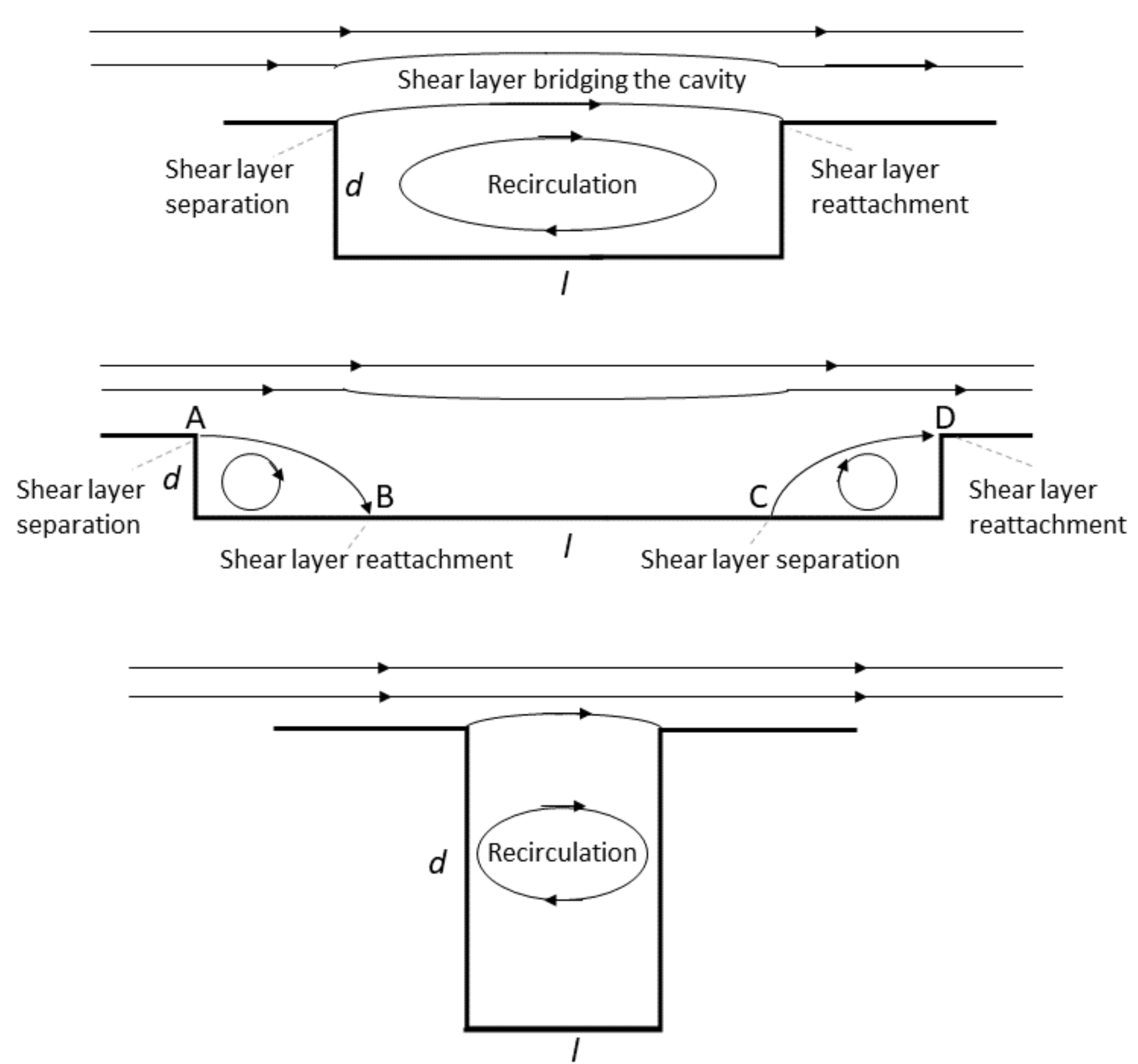
2.1. Passive Odor Sources

As described by the odor guidelines of Region Lombardy [21], wastewater tanks are passive sources because they are not characterized by their own volumetric flow. Their emissions are typically characterized through a specific odor emission rate (SOER), expressed in ouE/m²/s. The SOER is determined by the product of the odor concentration (C_Od, ouE/m³) and the volumetric flow rate (Q, m³/s) within the sampling device, divided by its area (A_B, m²):

$$SOER=\frac{Q C_{Od}}{A_B}$$

(1)

The odor emission rate (OER) in ouE/s is determined by the product of the SOER and the surface of the emitting source (A, m²):

$$OE{R}_R=SOER A$$

(2)

Subscript R in the previous equation indicates that the odor emission rate refers to the reference air speed (v_R, m/s) within the sampling device (e.g., a wind tunnel). Since the flow rate is a function of the air speed within the sampling device, when simulating odor emissions, one must consider the wind speed over the source area. As indicated by [22], the odor emission rate over the emitting surface (OER_S) can be calculated as:

$$OE{R}_S=OE{R}_R {\left(\frac{v_S}{v_R}\right)}^{\gamma }$$

(3)

where γ is 0.63 in [22] and 0.5 in [21]. The value of γ indicated by the odor guidelines of Region Lombardy [21] is used in this paper. In the previous equation v_s (m/s) is the wind speed close to the surface of the odor source, and it can be calculated with a power law profile as

$$v_S=v_h {\left(\frac{z}{h}\right)}^{\beta }$$

(4)

where h (m) is the anemometer height-or the height at which a meteorological model provides the wind speed v_h (m/s), and z (m) is the height at which the wind is estimated.

The coefficient β depends on the atmospheric stability and terrain type of the area of application (rural or urban). Different values have been proposed for the coefficient β (e.g., [23,24]). In the following, the default values of the old ISC3 dispersion model [25] will be used; they are summarized in

Table 1. Values of β in predicting the wind speed profile.

Stability Class	Rural Terrain	Urban Terrain
A	0.07	0.15
B	0.07	0.15
C	0.10	0.20
D	0.15	0.25
E	0.35	0.30
F	0.55	0.30

.

Ravina et al. (2020) [8] discussed the use of three different relations to downscale the wind speed at the height of interest: the power law (Equation (4)), the logarithmic law of the similarity theory and the Deaves–Harris law [17]. Depending on the relation used, they found significant differences in the resulting odor impact. However, for the purposes of this work, the power law profile (Equation (4)) will be used.

The tank height above the ground is typically used for z in Equation (4). This assumption is correct when the tank is full or almost full, while it can give rise to emission overestimation when the tank is not completely full. In fact, when z is the tank height, v_s in Equation (4) represents the wind speed at the top of the tank; however, it is typically higher than the wind speed close to the emitting surface, which is responsible for “stripping” the odorous molecules. On the other hand, assuming z equal to the height of the emitting surface is not correct when the surface is well within the tank.

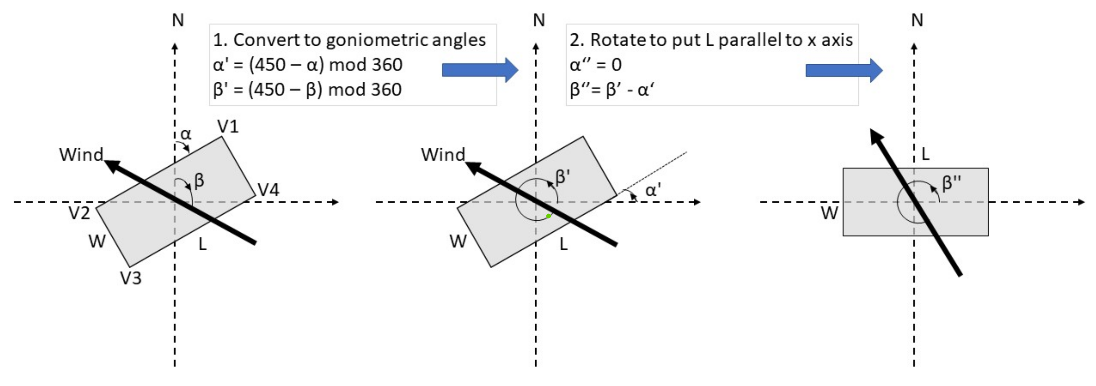
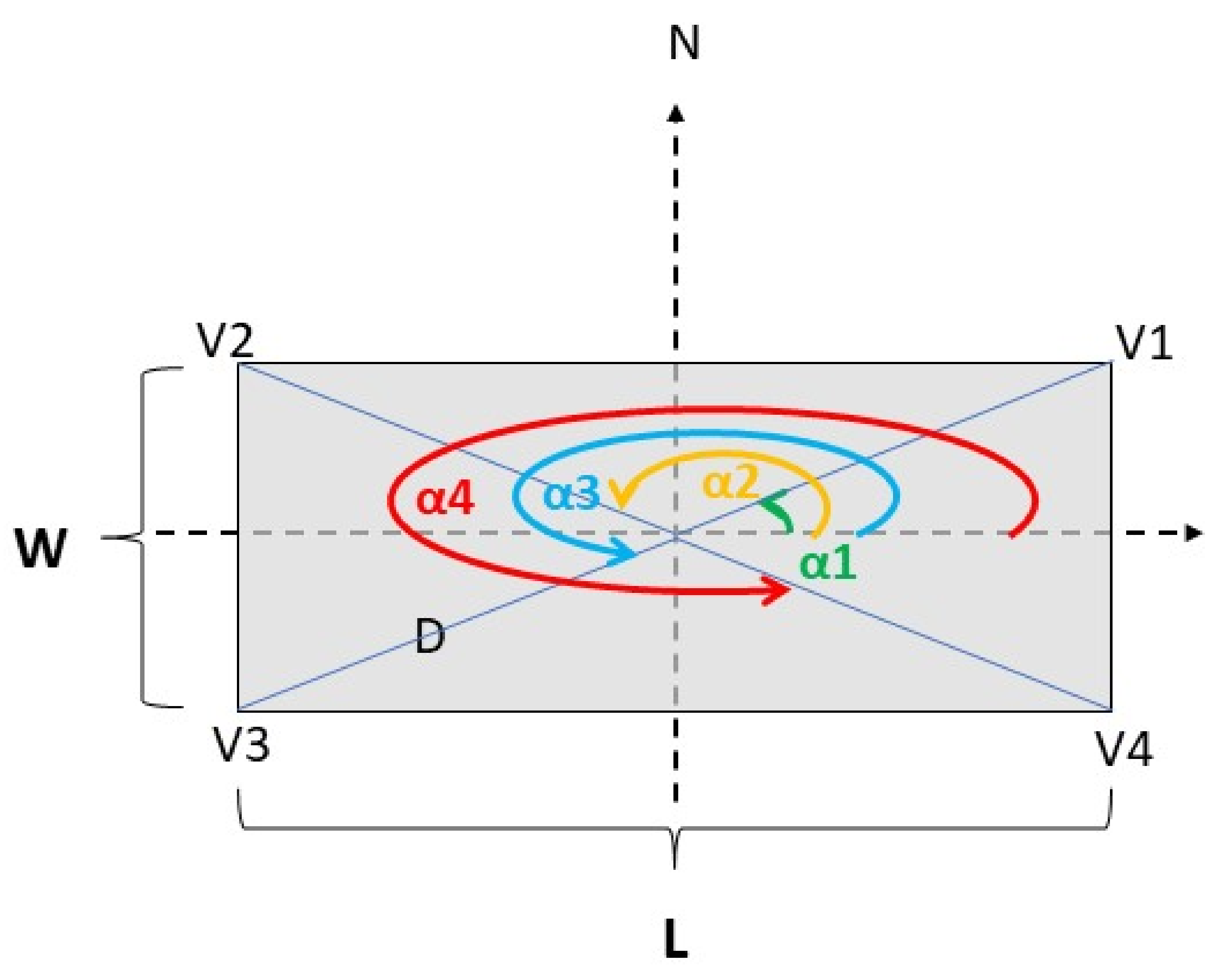
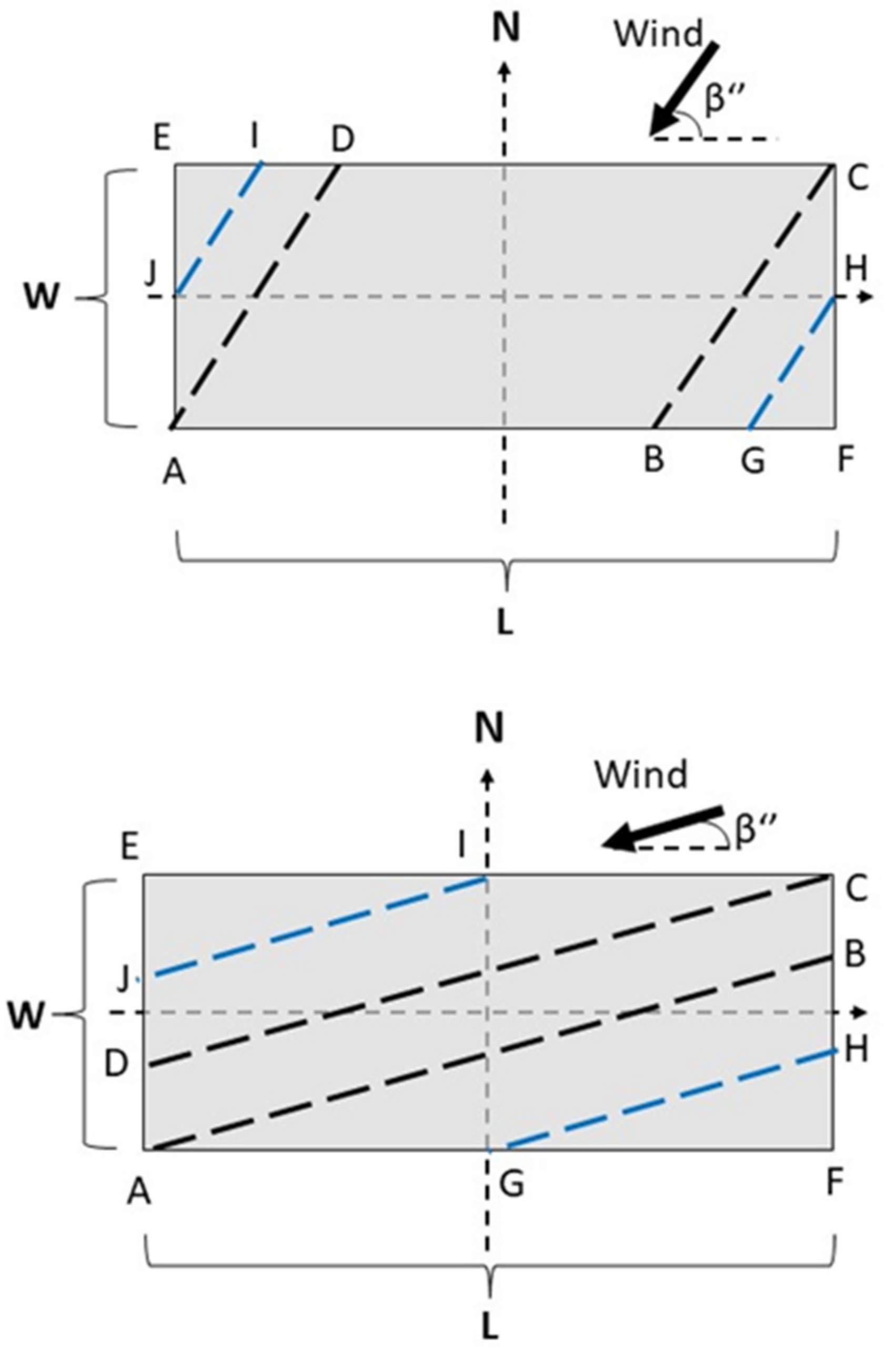
2.2. Wind Speed over the Emitting Surface

As far as the authors are aware, there are no simple expressions (i.e., analytical solutions of a complex set of equations) describing the wind flow within an open roof tank. The problem of a rectangular tank with the emitting surface at a certain distance from its top has some similarities with the problem of the street canyon, for which analytical solutions have been proposed.

For example, Soulhac et al. (2008) [26] presented an analytical solution for the wind flow within a street canyon when the external wind is parallel to the street. Hotchkiss and Harlow (1973) [27] found an analytical solution capable of determining the wind components at any point within a street canyon on a plane perpendicular to its longitudinal axis. Yamartino and Wiegand (1986) [28] found a reasonable agreement between the wind measurements in a street canyon with H/W close to 1 (where H is the height of the buildings and W is the width of the street) and the solution proposed by Hotchkiss and Harlow. Unfortunately, the solution is valid only for external wind that is perpendicular to the street. Berkowicz et al. (1997) [29] proposed a simple expression to estimate the average wind speed at street level.

In addition to the similarities, there are also differences between the street canyon problem and the rectangular tank problem. The main difference between them is the assumption of an infinitely long street, which may be justified when L >> W, where L is the street length and W is the width. While this assumption may be reasonable in most streets, it might be not reasonable in rectangular tanks; therefore, the street canyon analogy has not been further explored.

Open roof rectangular tanks may be considered as cavities, which have been deeply studied, for example in the automotive and aerospace sectors, mainly because they are responsible for noise production (e.g., [30]). Cavities may be classified according to their length-to depth (l/d) ratio: cavities with l/d < 1 are classified as deep, while those with l/d > 1 are classified as shallow [31]. Three different flow types can originate within cavities according to their l/d ratio [32]:

1 < l/d < 6-7: An open flow type is present within a shallow cavity. It is characterized by a large recirculation zone within the cavity and a shear layer bridging the entire cavity. The shear layer separates the cavity internal flow and the freestream flow outside the cavity (Figure 1. top).

l/d > 8-9: A closed flow type is present within the shallow cavity. Under this condition, on the leeward side, the shear layer separates at the edge of the cavity (separation point, A), and then hits the cavity floor (impingement point, B). Then, the shear layer detaches from the floor (separation point, C) and flows over the windward side of the cavity (stagnation point, D). Two recirculation zones form: one between the separation point A on the leeward side and the impingement point B, the other between the separation point C within the cavity and the stagnation point D. A schematic representation of a closed cavity flow is shown in Figure 1 (center). In this situation, a considerable part of the emitting surface (the one between the impingement point B and the separation point C) is characterized by the same wind speed that is present at the top of the tank.

l/d < 1: An open flow type is present within the deep cavity. A net separation exists between the flow within the cavity and freestream flow (Figure 1. bottom). Recirculation flow in these open flow deep cavities is not as strong as in the shallow ones.

The reader must be aware that Figure 1 is only a simple schematization of the flow types that may happen within a cavity; it is not to scale and does not reproduce all the peculiarities of the flows. The value of the ratio l/d in a shallow cavity for the transition from open flow to closed flow is not so sharp. Additionally, a so-called transitional flow originates within the cavity during the passage. For simplicity, we will neglect the transitional flow and consider the transition from an open to closed flow when l/d = 7.

The rectangular tank represented in Figure 2 is considered, where W and L are the tank width and length (W ≤ L), respectively, α is the orientation of the longest side of the tank (i.e., considering L, not W) with respect to north, and DTL is the distance between the tank top and emitting surface.

Keeping in mind the analogy with cavities, in order to describe the average ventilation above the emitting surface, three situations are defined by considering DTL for d and the projection of the open roof rectangular tank along the wind direction (i.e., the path, P, of the wind over the emitting surface, as described by the following Equations (7) and (8)) for l:

Open flow in deep cavities (P/DTL < 1). It is assumed that the ambient wind does not reach the emitting surface, because it does not have sufficient space to enter within the tank; thus, the emissions will not depend on the wind speed. In this situation, it is assumed that OER = OER_R, without any correction for wind speed or wind direction.

Open flow in shallow cavities (1 < P/DTL < 7). In general, large values of the DTL should hinder the circulation of air within the tank and, thus, reduce the odor emissions from the liquid surface. Therefore, the average wind speed above the emitting surface (v_L) must decrease as the distance DTL increases. It is assumed that v_L can be described with a logarithmic profile, as done, for example, by [29] within a street canyon:

$$v_L=\mathsf{\mu } v_S \frac{ln\left(\raisebox{1ex}{$h_0$}\!\left/ \!\raisebox{-1ex}{$z_0$}\right.\right)}{ln\left(\raisebox{1ex}{$DTL$}\!\left/ \!\raisebox{-1ex}{$z_0$}\right.\right)}$$

(5)

In the previous expression, h₀ is the height above the odor-emitting surface at which the wind speed is evaluated; in the following calculations, it is set to 0.1 m. For the roughness length z_0, a value of 0.01 m is used, assuming a mud-like surface. This roughness length value was chosen considering, for example, a manure tank or an aerobic sludge digestion tank. Of course, the value may be different when the tank contains mainly water. An estimate of the uncertainties due to the choice of z₀ and other variables is reported in paragraph 3.4.

The correction factor μ is equal to 0.8. This is determined from the correction factor used in [29] for street canyons: μ = (1−0.2 p sin(φ)), where φ = 0 for a wind parallel to the street canyon, and p is the ratio between the street canyon height upwind and its average height (in our case p = 1). For a rectangular tank, the concept of parallel wind speed is not applicable, since the infinite length assumption is not realistic, therefore, we assume sin(φ) = 1, and then μ = 0.8. When the DTL is relatively small, there should be little or no variation between the external wind and v_L. For this reason, the wind speed correction should be applied only when the DTL exceeds a certain threshold value, for example when the DTL > h₀. When the DTL is smaller than such a value, it is assumed that the wind speed does not change (i.e., the value at tank top is used).

Closed flow in shallow cavities (P/DTL > 7). It is assumed that the average wind speed within the two recirculation zones can be calculated with the logarithmic profile, as for the open flow in shallow cavities (Equation (5)), while between the impingement and the detachment points, the external wind speed is considered. The distance of the impingement point from the leading edge increases with the depth of the cavity, as the distance from the separation point and the trailing edge. We assume that each one of the two distances is proportional to DTL through a factor k, therefore, excluding a length equal to 2 k DTL, the remaining length is characterized by the external wind speed. Then, the average speed over the emitting surface is given by a linear combination:

$$v_L=\frac{v_S}{\left(\raisebox{1ex}{$P$}\!\left/ \!\raisebox{-1ex}{$DTL$}\right.\right) } \left[2 k \mathsf{\mu } \frac{ln\left(\raisebox{1ex}{$h_0$}\!\left/ \!\raisebox{-1ex}{$z_0$}\right.\right)}{ln\left(\raisebox{1ex}{$DTL$}\!\left/ \!\raisebox{-1ex}{$z_0$}\right.\right)}+\left(\raisebox{1ex}{$P$}\!\left/ \!\raisebox{-1ex}{$DTL$}\right.-2 k\right) \right]$$

(6)

In this work, k = 3 was used. Additional work is needed to evaluate the correctness of this arbitrary choice.

The wind path (P) over the emitting surface can be calculated as shown in Figure 3 (wind vector entering and exiting through L) and Figure 4 (wind vector entering and exiting through W). The tank orientation with respect to the north is α, while the wind direction is β. The goniometric angles to the segments formed by joining the rectangle center with its vertexes are α1, α2, α3 and α4. If D is half the rectangle diagonal, calculated with the Pythagoras theorem starting from L and W, the four limiting angles corresponding to the vertexes can be calculated by defining γ = arcsin(W/(2D)), and then, after rotating the tank (Figure 5), α1 = γ, α2 = 180 − γ, α3 = 180 + γ and α4 = 360 − γ. The wind enters and exits through L when α1 < β″ < α2 or α3 < β″ < α4, while it enters and exits through W when α4 < β″ < α1 or α2 < β″ < α3 (thus, the name limiting angles).

Then, after converting the tank orientation and wind direction from north to goniometric angles, and after rotating the tank (all equations shown in Figure 3 and Figure 4), the following relation can be used for calculating the wind path P over the tank when the wind vector enters and exits through its longest size L (Figure 3):

$$P=\left|\frac{W}{sin\left({\beta }^{″}\right)}\right|$$

(7)

On the contrary, when the wind vector enters and exits through the shortest size of the tank W (Figure 4), the following equation can be used:

$$P=\left|\frac{L}{cos\left({\beta }^{″}\right)}\right|$$

(8)

P is the maximum path that wind has over the tank, and it does not affect the whole area but only part of it. For example, considering Figure 6 (top), when the wind vector enters and exits through L, the path P is equal to BC (or AD), and it sweeps the parallelogram ABCD, while the wind path over the triangles BFC and ADE is shorter. For those triangles, an average path Pa passing in W/2 is considered, with Pa = GH = IJ = abs(W/(2 sin(β″))) = P/2.

Then, P is used for the area of the parallelogram, equal to W (L-P cos(β″)), while Pa is used for the sum of the areas of the triangles, equal to PW cos(β″). Similarly, when the wind vector enters and exits through W (Figure 6, bottom), the path P is equal to AB (or CD), and it sweeps the parallelogram ABCD, while the wind path over the triangles AFB and DCE is shorter. For those triangles an average path Pa passing in L/2 is considered, with Pa = GH = IJ = abs (L/(2 cos(β″))) = P/2. Then, P is used for the area of the parallelogram, equal to L (W-P sin(β″)), while Pa is used for the sum of the areas of the triangles, equal to PL sin(β″).

Therefore, at each time, the odor emissions from the tank are calculated as the sum of the contribution of the parallelogram and the contribution of the rectangle obtained from the sum of the two triangles.

2.3. The LAPMOD Dispersion Model

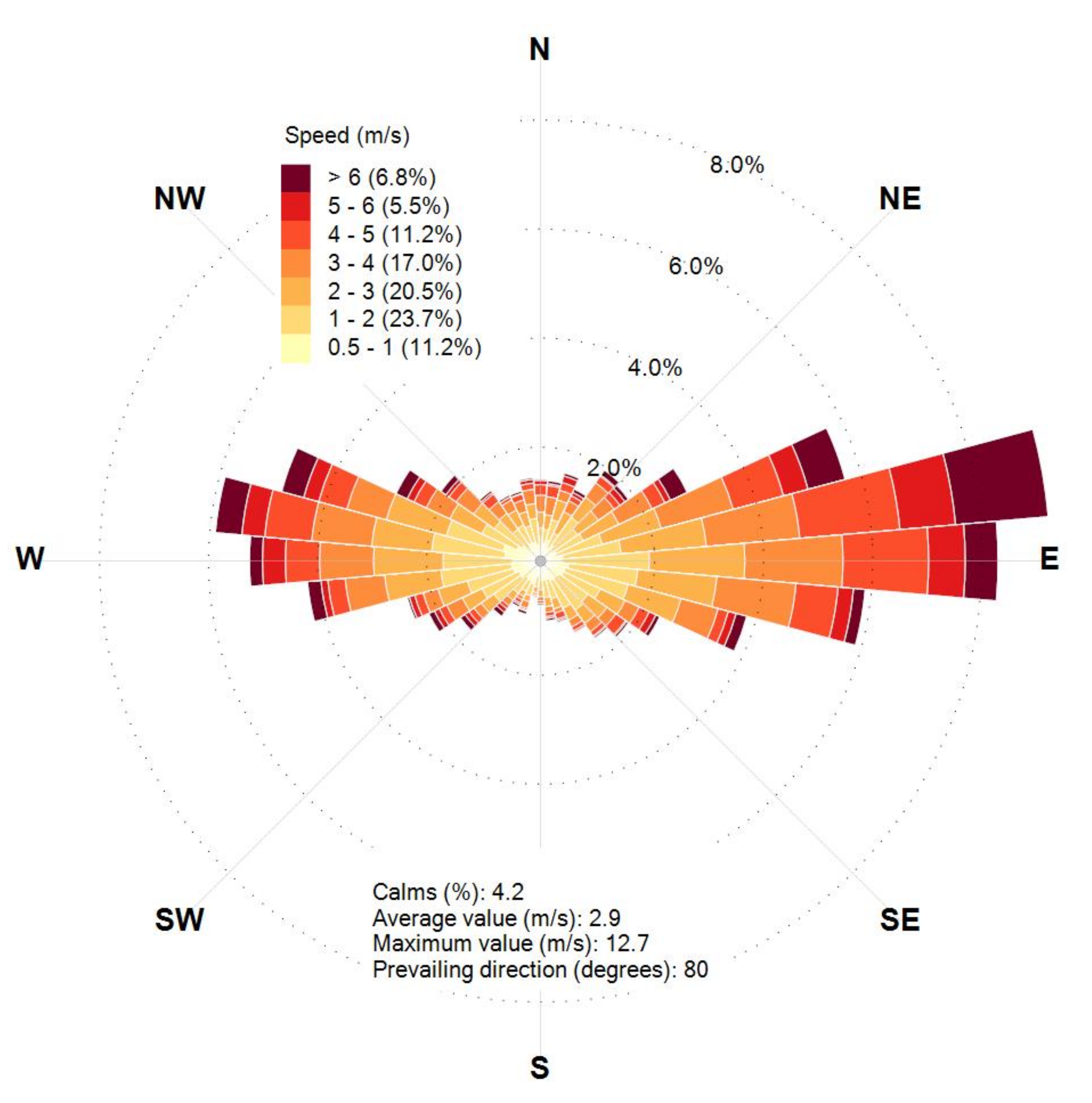
The LAPMOD modeling system is an open-source Fortran code available at https://www.enviroware.com/lapmod (accessed on 19 February 2022). The model has been described in [19,20]; the same papers also describe the model validation against two experimental datasets: one in rural terrain (Kincaid) and one in urban terrain (Indianapolis).

According to the performance evaluation criteria proposed by [33]–based on FA2, NMSE and fractional bias–LAPMOD can be defined a reliable model in both terrain types. Since model validation is a continuous process, other tests are underway. Another validation was described by [34], while an intercomparison with other models for odor applications was described by [35].

LAPMOD calculates the concentration fields with different kernel methods [36]. For odor modeling applications, peak concentrations can be calculated in two ways by LAPMOD according to the user’s choice: (1) by applying a constant peak-to-mean factor to the 1-h average concentration (for example 2.3 as indicated in [21]) or (2) as a function of the atmospheric stability and distance from the source, as described in [37]. This second method for determining the peak concentration is more realistic with respect to the application of a constant peak-to mean factor applied to the 1-h average concentration.

A comparison among three methods for calculating the peak concentrations was recently described in [5]. In this work, the peak concentrations are determined as a function of atmospheric stability and distance from the source, as described in [37] and specifically summarized for LAPMOD in [35]. Concentrations were calculated starting from the particles positions with the Uliasz parabolic kernel [19].

2.4. Meteorology

LAPMOD was fed by the meteorological field prepared with the Weather Research and Forecasting model (WRF) [38] and CALMET [23]. WRF is a mesoscale numerical weather prediction system designed for both atmospheric research and operational forecasting. CALMET is a diagnostic meteorological model that reconstructs the 3D wind and temperature fields and micrometeorological variables (e.g., mixing height, Monin-Obukhov length, friction and convection velocity) starting from meteorological measurements and/or output of prognostic model and geophysical data (orography and land use).

WRF (version 3.9.1, ARW core) was initialized with the NCEP FNL (Final) Operational Global Analysis data (https://rda.ucar.edu/datasets/ds083.2/ (accessed on 19 February 2022)), operationally prepared every 6 h on a 1 × 1 degrees grid. The NCEP FNL dataset includes many observational data. WRF was run at 45 vertical levels, up to 50 mb, and a three-level domain nesting was used, with domain resolution of 27, 9 and 3 km, respectively.

CALMET (version 6.5.0, level 150223) was employed on a domain of 14 × 14 km², with a grid resolution of 200 m. The WRF output of its innermost domain was used in input by CALMET as surface and upper air data. The 1-h CALMET output data of the computational grid containing the source were extracted for the whole simulation year (2020). These data are used in input by the emission processor implementing the equations described in the previous sections. They were also used to prepare the wind rose shown in Figure 7.

2.5. Source Term

Four hypothetical open-roof rectangular tanks with a surface of 90 m² and different shape factors (L/W) were considered (

Table 2. The sizes of the four tanks.

Tank	Length (m)	Width (m)	L/W
L10_W9	10.0	9.0	1.11
L12_W7.5	12.0	7.5	1.60
L15_W6	15.0	6.0	2.50
L18_W5	18.0	5.0	3.60

). All the tanks had a height of 3 m above the ground and the same centroid. For each tank, two different orientations (90 and 180 degrees) and four DTLs were considered, as summarized in

Table 3. Common characteristics of the fictitious tanks.

Parameter	Value
Height (m)	3
DTLs (m)	0.0, 0.5, 1.0, 1.5
Orientations (degrees)	90, 180
SOER (ouE/m2/s)	80

. As already specified, DTL means the distance between the tank top and the emitting surface within the tank (see Figure 2).

The tanks were located in a region of the northern part of Italy, within the Po Valley, which, in many places, is characterized by prevailing winds from east to west and vice versa (see Figure 7). For this reason, in order to show the two most different effects, two orientations are considered in Table 3: one with the longest size of the tank more or less parallel to the prevailing winds (90 degrees) and one with the longest size of the tank perpendicular to the prevailing winds (180 degrees). Tank orientation is measured as the wind direction: north is zero, and the angle increases clockwise. The SOER value reported in Table 3 may be representative, for example, for an aerobic sludge digestion tank.

For each tank, eight emission scenarios result from the combination of the tank orientations and DTLs described in Table 3. The simulations with DTL = 0 m represent the base case scenarios, and their emissions were obtained with Equation (3) without considering the wind direction and the location of the emitting surface within the tank.

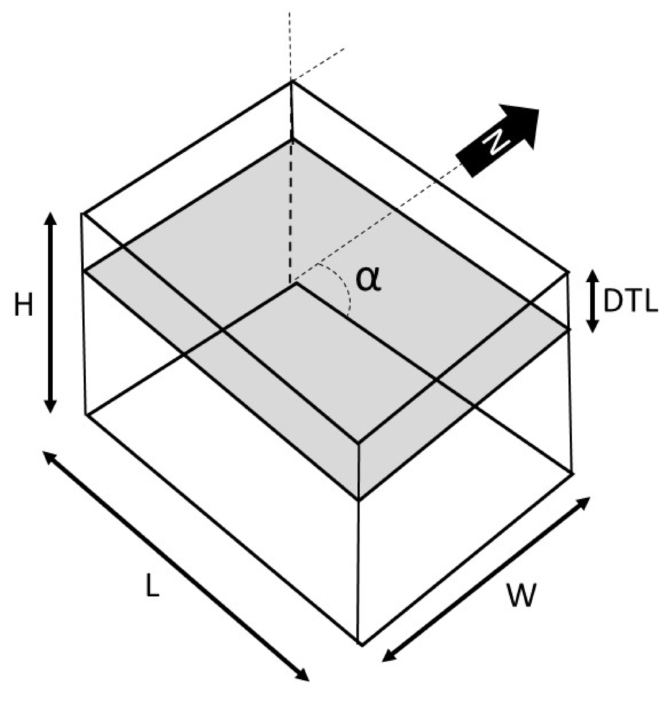
2.6. Simulation Domain

The output concentrations were calculated both on regular receptors placed on a Cartesian grid and on discrete receptors. Regular receptors were placed over a square domain of 6 × 6 km² with a distance of 50 m from each other. Discrete receptors were placed at the intersections of two circles (centered over the common centroids of the sources with radius of 500 m and 1000 m) with the segments exiting from the centroid of the sources with angles from 0 to 360 degrees with steps of 45 degrees (where 0 degrees is north). Therefore, a total of 16 discrete receptors was used. All the receptors, regular and discrete, were placed 2 m above ground level.

3. Results and Discussion

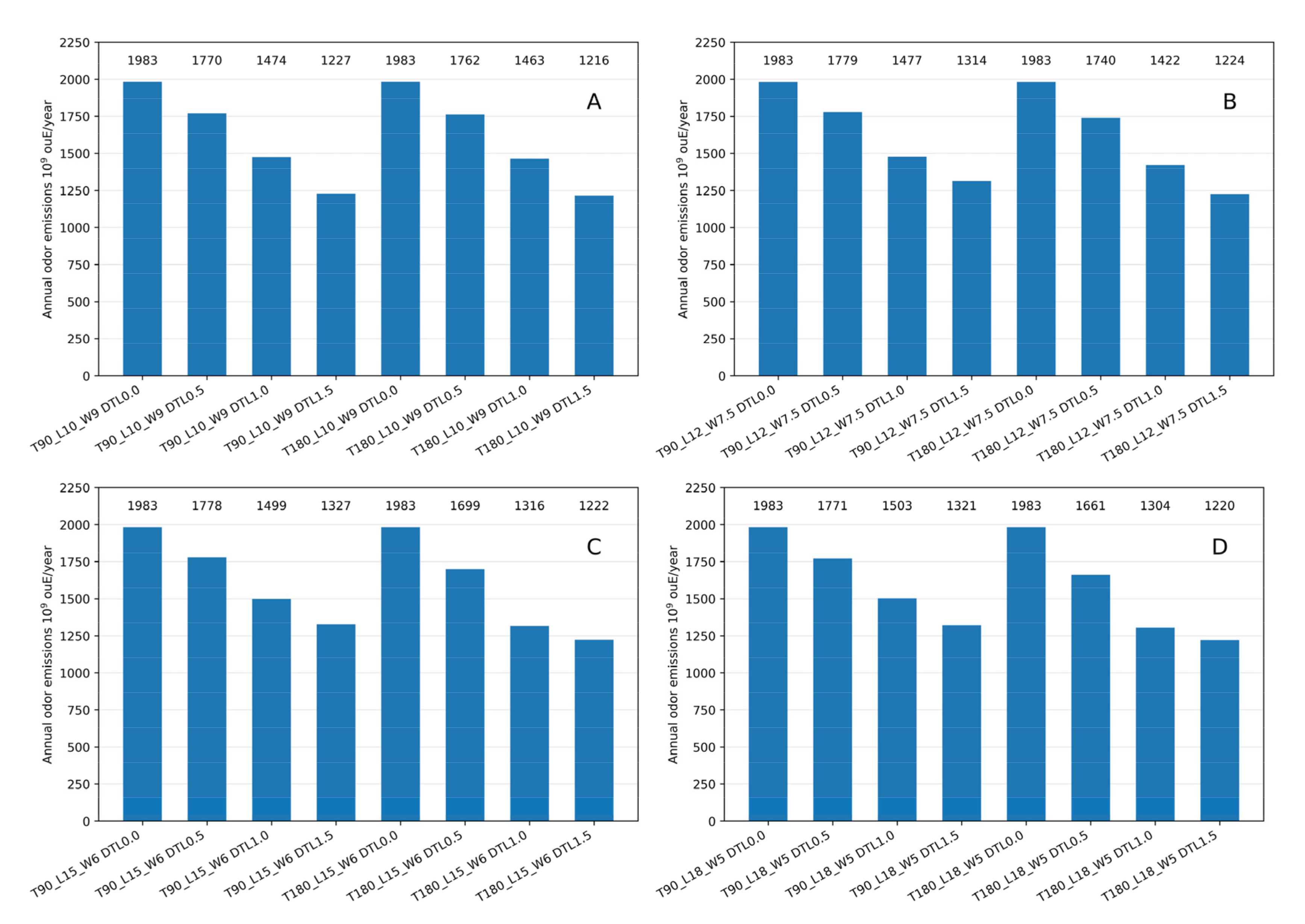
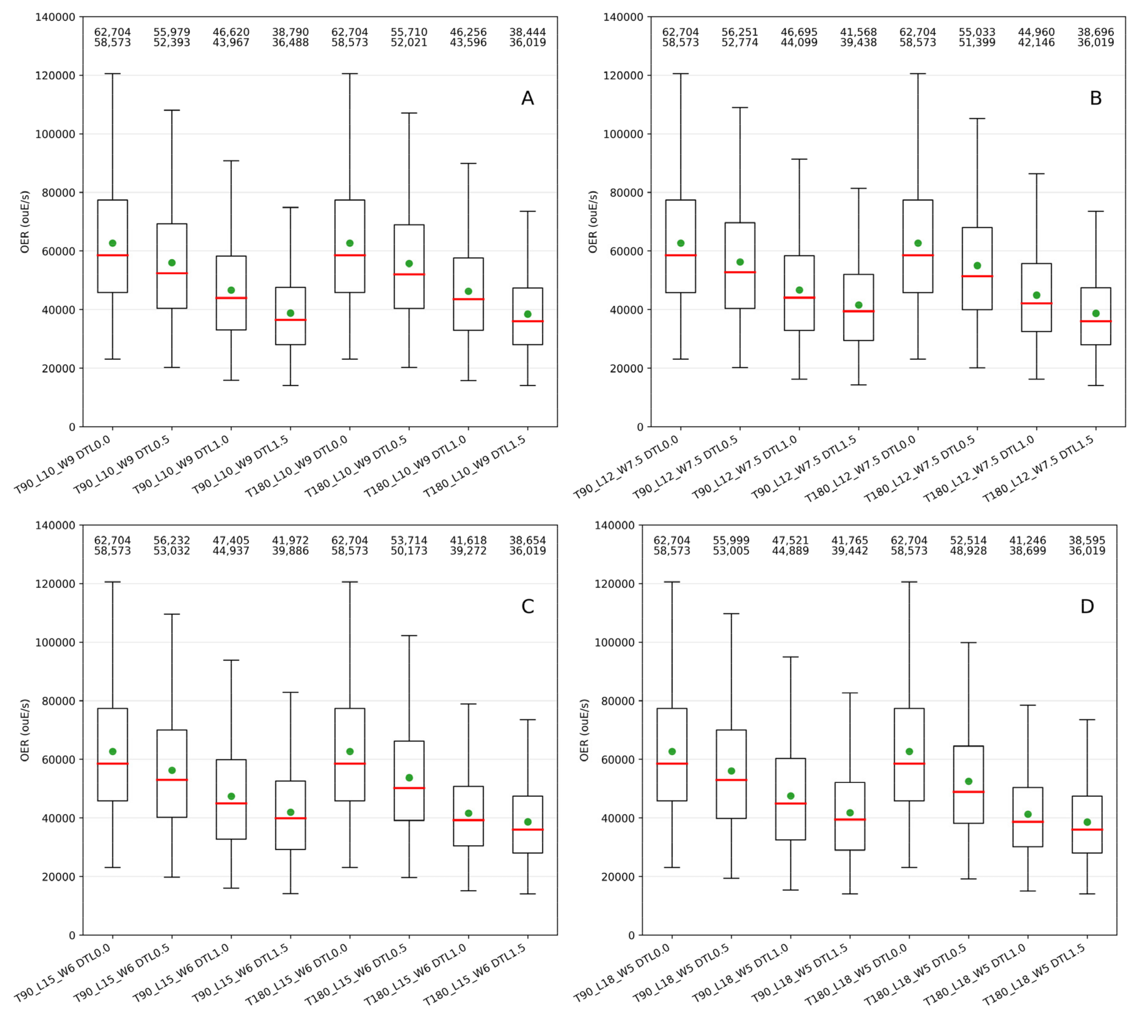
As already stated, the simple heuristic approach described for estimating odor emissions must be verified and, perhaps, modified by means of CFD simulations and/or experimental testing. Liu et al. (1995) [18], for example, in their Figure 5, showed that the wind speed profile within an almost empty tank with W/H = 2, at its center, had a sigmoidal shape.

Additionally, by sticking with the street canyon profile, the analytical expressions proposed by Hotchkiss and Harlow (1973) [27] to solve the vorticity equation show that, for large canyons (W/H = 2), the average wind at the bottom is similar to that at the top, with minimum values at mid height corresponding to the center of the flow rotor. Then, in this situation the wind speed is not a monotonic function of the DTL (as instead Equation (6) is), because it decreases up to a minimum, and then it increases again. However, the Hotchkiss and Harlow equations also show that, for narrower canyons (W/H = 1 or W/H = 0.5), the average wind speed decreases by increasing the distance from the top of the buildings (i.e., by increasing DTL in our case).

Keeping in mind these uncertainties, LAPMOD was used for calculating the separation distances as a function of different tank orientations and DTLs and to evaluate odor concentrations.

3.1. Emissions

The annual odor emissions resulting from the different scenarios are illustrated in Figure 8. The label reported for each bar indicates the tank configuration and orientation; for example, T90_L15_W6_DTL0.5 indicates tank L15_W6 (see Table 2) with orientation 90 degrees and DTL = 0.5 m. As shown, the base case (i.e., DTL = 0.0 m) emissions are the same for all the tanks independently from their orientations. On the contrary, when DTL ≠ 0.0 m and the tank has an orientation of 90 degrees–i.e., its longest size is aligned to the prevailing wind–the annual emissions are always larger than those determined for a tank with 180 degrees orientation, and the difference increases as the shape factor increases.

This does not mean that the emissions of the 90 degrees tank are always larger than those of the 180 degrees tank at any hour, since they depend on wind direction and wind speed at that specific hour. The relative variations of the total odor emissions, expressed as percentages, are summarized in

Table 4. Relative percent variation of the total emissions.

DTL (m)	L10_W9 (%)	L12_W7.5 (%)	L15_W6 (%)	L18_W5 (%)
0.0	0.0	0.0	0.0	0.0
0.5	0.5	2.2	4.5	6.2
1.0	0.8	3.7	12.2	13.2
1.5	0.9	6.9	7.9	7.6

. For any specific DTL value, relative variations are calculated as the difference between total emissions of the 90-degree and 180-degree tank, divided by the total emissions of the 90-degree tank.

Table 4 shows that, when the shape factor is 1.11 (tank L10_W9, Figure 8A), there is practically no difference between the emissions when the tank has two different orientations: the largest variation is 0.9% when the DTL = 1.5 m. When the shape factor is 1.6 (tank L12_W7.5, Figure 8B), the relative variation for different tank orientations increases with the DTL up to a maximum of 6.9% when the DTL = 1.5 m. For the other two shape factors (2.5 for L15_W6, Figure 8C and 3.6 for L18_W5, Figure 8D), the relative variation is larger for DTL = 1 m than for DTL = 1.5 m.

Moreover, the relative variation when DTL = 1.5 m is smaller when the shape factor is 3.6 than when it is 2.5. This apparently awkward behavior is due to the fact that wind speed variation over the emitting surface passing from a shallow-cavity closed-flow to a shallow-cavity open-flow is larger with respect to the wind variation remaining in a shallow-cavity open-flow. For example, when tank L15_W6 has an orientation of 180 degrees, the wind is often more or less perpendicular to it. If we consider, for simplicity, a wind that is perfectly perpendicular, its path over the tank is 6 m long. Therefore, when DTL = 0.5 m (P/DTL = 12: shallow-cavity closed-flow), the wind speed over the emitting surface is calculated with Equation (6).

On the contrary, when DTL = 1 m (P/DTL = 6: shallow-cavity open-flow), the wind speed over the emitting surface is calculated with Equation (5). Finally, when DTL = 1.5 m (P/DTL = 4: shallow-cavity open-flow), the wind speed over the emitting surface is again calculated with Equation (5). In this situation, the wind speed variation passing from DTL = 0.5 m to DTL = 1.0 m is larger than the wind speed variation passing from DTL = 1.0 m to DTL = 1.5 m. As a consequence, the emission variation passing from DTL = 0.5 m to DTL = 1.0 m is larger than the emission variation passing from DTL = 1.0 m to DTL = 1.5 m.

The distribution of the odor emission rates (OERs) of the different tanks and scenarios is represented in Figure 9 with a box-and-whiskers plot. The red segments show the median value, while the green circles represent the mean values of each OER distribution. The height of each rectangle represents the interquartile range of the distribution (i.e., the difference between the values representing the 75th and the 25th percentiles), while the small horizontal segments at the extremes represent the 2nd percentile and the 98th percentile of the distribution.

The OER distributions when DTL = 0.0 m are identical, while, for a fixed tank orientation, the mean, median and 98th percentile decrease increasing the DTL value. Excluding tank L10_W9 (Figure 9A), for which the values vary more or less in the same way as a function of the DTL for the two orientations, the mean, median and 98th percentile for the 180-degree tank are always smaller than those of the 90-degree tank for the same DTL.

In order to evaluate, in more detail, the effects of wind direction, the emissions of tank L18_W5 with the two different orientations were analyzed when wind blew from the intervals (345, 15) degrees or (165, 195) degrees and when it blew from the intervals (75–105) degrees and (255–285) degrees. Practically, an arc of 30 degrees was considered–the amplitude of the arc from the center of the tank to its smaller side–from north, south, east and west.

Due to the specific wind rose of this study (Figure 7), there were 632 events when wind blew from north or south and 3488 events when it blew from east or west. The maximum OER calculated for tank L18_W5 with different orientations and for different DTLs is summarized in

Table 5. Maximum OER (ouE/s) calculated for different wind directions.

Tank	Wind from N or S	Wind from E or W	Ratio
T90_L18_W5 DTL0.5	120,431	132,688	1.10
T180_L18_W5 DTL0.5	135,547	115,769	0.85
T90_L18_W5 DTL1.0	92,659	121,976	1.32
T180_L18_W5 DTL1.0	120,043	88,844	0.74
T90_L18_W5 DTL1.5	88,831	109,379	1.23
T180_L18_W5 DTL1.5	100,162	85,174	0.85

. The ratio between the values calculated when wind blows from east or west and when the wind blows from north or south (the rightmost column of Table 5) clearly show the effect of the tank orientation.

When the tank had a 90 degrees orientation, the maximum OER was greater for easterly or westerly winds than for northerly or southerly winds. On the contrary, when the tank had a 180-degree orientation, the maximum OER was greater for northerly or southerly winds than for easterly or westerly winds. The combined effect of wind direction and tank orientation is also visible, although less evident for the different number of events, for the average emission when the wind blows from the four specified directions in

Table 6. Average OER (ouE/s) calculated for different wind directions.

Tank	Wind from N or S	Wind from E or W	Ratio
T90_L18_W5 DTL0.5	44,425	64,633	1.45
T180_L18_W5 DTL0.5	50,364	56,966	1.13
T90_L18_W5 DTL1.0	34,138	58,231	1.71
T180_L18_W5 DTL1.0	45,301	43,770	0.97
T90_L18_W5 DTL1.5	32,728	50,221	1.53
T180_L18_W5 DTL1.5	38,940	41,962	1.08

.

In any case, even for the averages, the emission ratios depend on the tank orientation and wind direction. The impacts of these emission scenarios over the surrounding environment were simulated for a whole year.

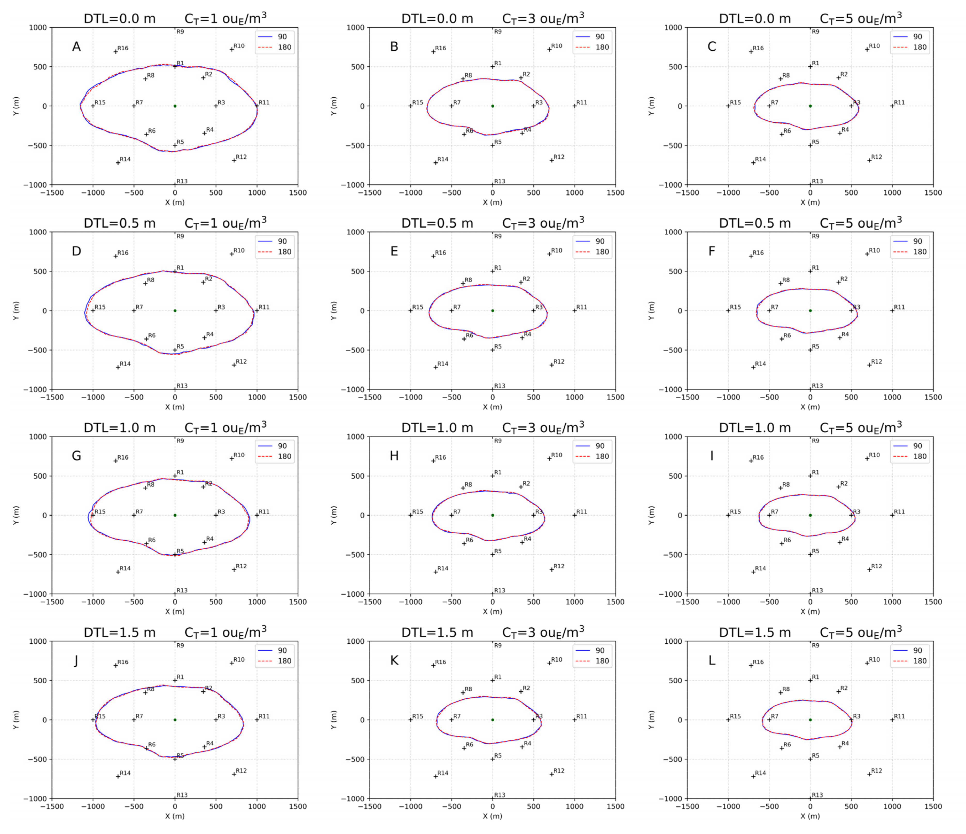
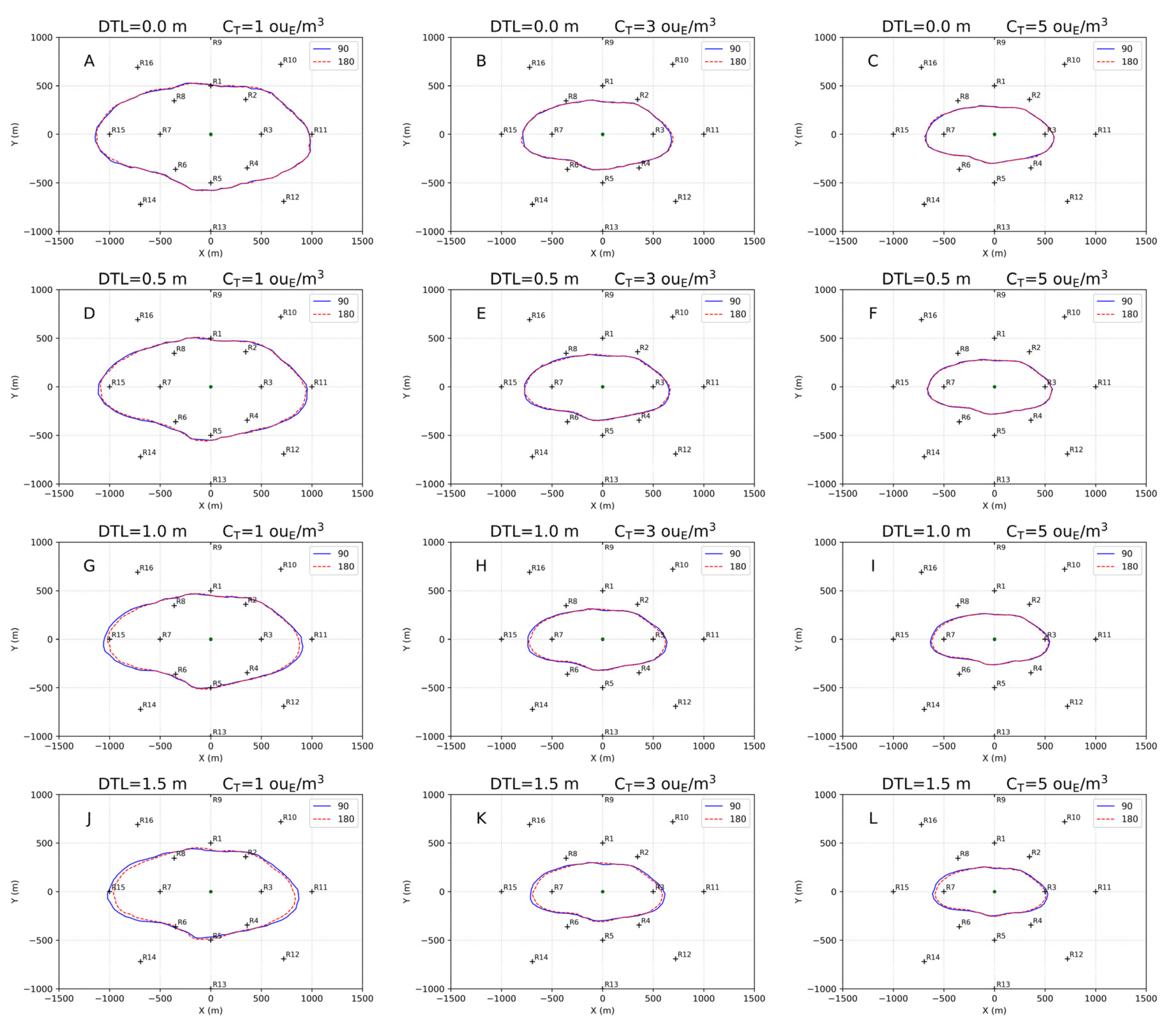
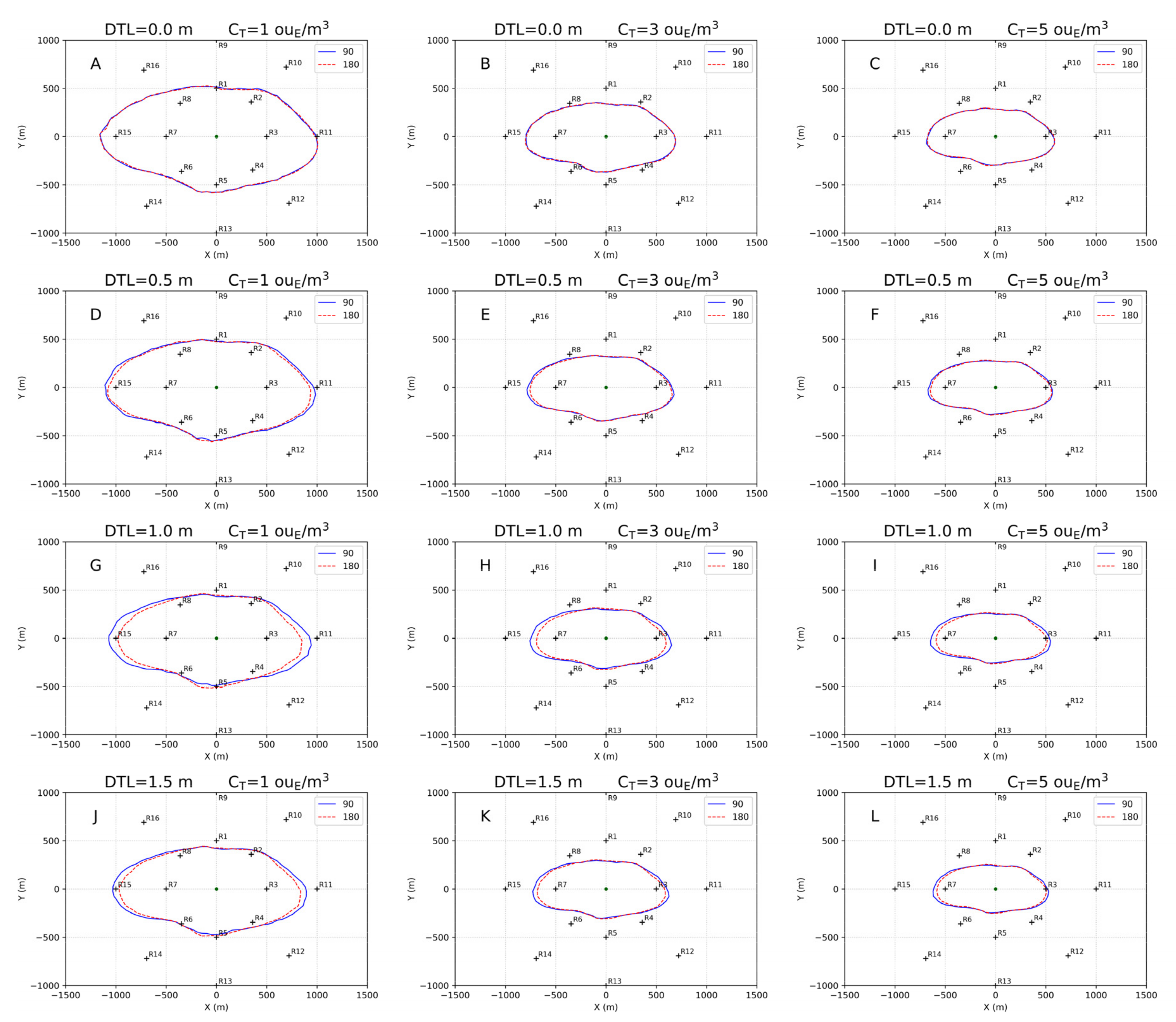
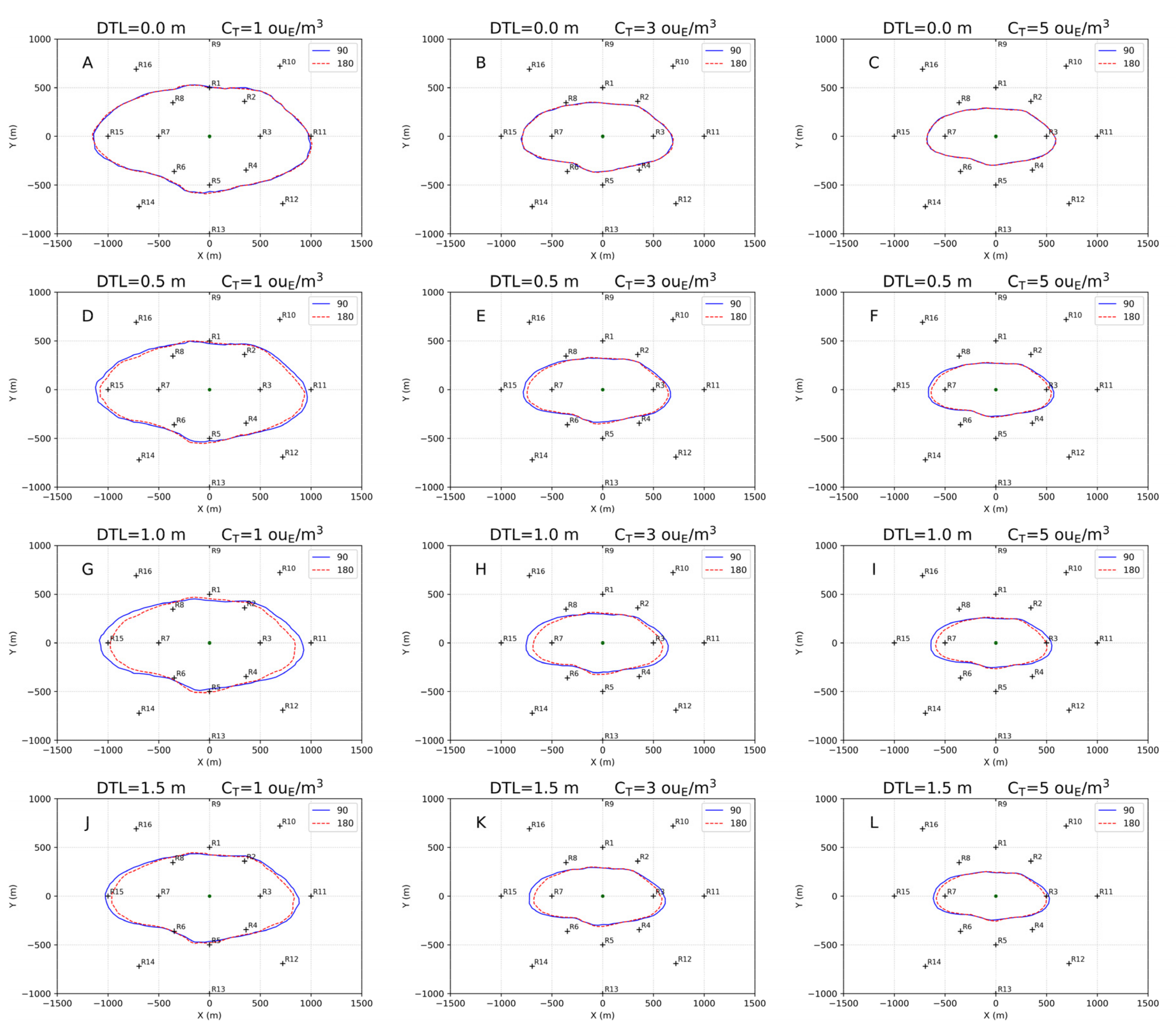
3.2. Separation Distances

Separation distances were calculated considering the odor impact criteria (OIC) defined by Region Lombardy [21]: odor concentration threshold levels of 1 ouE/m³, 3 ouE/m³ and 5 ouE/m³ and exceedance probability of 2%. In other words, the 98th percentile of the peak concentrations at any output point should be lower than the threshold levels. As pointed out by [35], separation distances are described by the contour lines of an ambient concentration threshold at a fixed exceedance probability of such a threshold. The exceedance probability of 2% corresponds to 176 h, since a leap-year (2020) was simulated.

The resulting separation distances are illustrated in Figure 10, Figure 11, Figure 12 and Figure 13, and all of them have a potato-like shape, in agreement with the wind rose shown in Figure 7. In each figure, the top row (images A, B and C) represents the results of the base case scenarios, i.e., the OER_S for two identical tanks with same area and shape factor (L/W), but different orientations, is calculated with Equation (3), which does not consider the wind direction and distance between the tank top and the emitting surface (DTL = 0.0 m).

In fact, the continuous blue line, representing the results for the tank with a 90 degrees orientation, and the dashed red line, representing the results for the tank with a 180 degrees orientation, are almost superimposed. There are small differences between the contours, which are more evident when the shape factor increases, due to the fact that some particles are emitted in different places when the tank is placed with the two different orientations; however, those differences are negligible.

On the contrary, the contour lines reported in each figure from the second to the fourth row show the effects of the wind direction and DTLs on the separation distances. Specifically, images D, E and F refer to DTL = 0.5 m, images G, H and I refer to DTL = 1.0 m, and images J, K and L refer to DTL = 1.5 m.

The relative variation of the maximum separation distance along X (ΔX) and along Y (ΔY) for a specific tank orientation as a function of the DTL with respect to DTL = 0.0 m is summarized in

Table 7. Relative variation (%) of the maximum separation distances along X and Y as a function of the DTL. Or. is tank orientation.

			CT = 1 ouE/m3		CT = 3 ouE/m3		CT = 5 ouE/m3
Tank	Or. (degrees)	DTL (m)	ΔX (%)	ΔY (%)	ΔX (%)	ΔY (%)	ΔX (%)	ΔY (%)
L10_W9	90	0.5	−4.3	−4.4	−3.1	−6.9	−2.7	−4.2
L10_W9	180	0.5	−7.0	−3.3	−3.1	−6.9	−2.7	−4.2
L10_W9	90	1.0	−9.1	−13.3	−8.5	−13.8	−8.2	−14.6
L10_W9	180	1.0	−11.8	−12.2	−8.5	−13.8	−8.2	−14.6
L10_W9	90	1.5	−16.0	−17.8	−14.6	−17.2	−14.5	−20.8
L10_W9	180	1.5	−16.0	−17.8	−14.6	−17.2	−14.5	−20.8
L12_W7.5	90	0.5	−2.7	−4.4	−2.3	−3.6	−3.6	−4.3
L12_W7.5	180	0.5	−4.3	−3.3	−2.3	−3.6	−3.6	−4.3
L12_W7.5	90	1.0	−7.6	−13.3	−6.2	−14.3	−7.2	−10.9
L12_W7.5	180	1.0	−11.4	−12.2	−8.5	−12.5	−9.0	−10.9
L12_W7.5	90	1.5	−10.8	−18.9	−10.1	−19.6	−10.8	−17.4
L12_W7.5	180	1.5	−16.2	−14.4	−13.2	−14.3	−15.3	−15.2
L15_W6	90	0.5	−4.8	−4.4	−0.8	−7.0	−1.8	−6.5
L15_W6	180	0.5	−7.0	−3.3	−4.7	−7.0	−5.4	−4.3
L15_W6	90	1.0	−7.5	−15.6	−5.4	−15.8	−5.4	−13.0
L15_W6	180	1.0	−15.5	−11.1	−14.0	−12.3	−13.5	−10.9
L15_W6	90	1.5	−10.7	−20.0	−8.5	−19.3	−9.0	−17.4
L15_W6	180	1.5	−16.6	−16.7	−14.0	−15.8	−14.4	−15.2
L18_W5	90	0.5	−1.6	−7.8	−2.3	−8.8	−1.8	−8.7
L18_W5	180	0.5	−5.9	−4.4	−7.7	−3.5	−6.4	−4.3
L18_W5	90	1.0	−4.9	−16.7	−5.4	−17.5	−5.5	−15.2
L18_W5	180	1.0	−14.6	−12.2	−14.6	−10.5	−12.7	−10.9
L18_W5	90	1.5	−9.7	−20.0	−9.2	−17.5	−9.1	−15.2
L18_W5	180	1.5	−15.7	−16.7	−15.4	−12.3	−13.6	−13.0

. This relative variation is calculated for each orientation as (D_T,DTL-D_T,0.0)/D_T,0.0 × 100, where D_T,DTL represents the maximum separation distance along X or Y for orientation T and a specific DTL, and D_T,0.0 represents the maximum separation distance along X or Y for orientation T and DTL = 0.0 m.

Similarly,

Table 8. Relative variation (%) of the maximum separation distances along X and Y as a function of the tank orientation.

		CT = 1 ouE/m3		CT = 3 ouE/m3		CT = 5 ouE/m3
Tank	DTL (m)	ΔX (%)	ΔY (%)	ΔX (%)	ΔY (%)	ΔX (%)	ΔY (%)
L10_W9	0.5	−2.8	1.2	0.0	0.0	0.0	0.0
L10_W9	1.0	−2.9	1.3	0.0	0.0	0.0	0.0
L10_W9	1.5	0.0	0.0	0.0	0.0	0.0	0.0
L12_W7.5	0.5	−1.7	1.2	0.0	0.0	0.0	0.0
L12_W7.5	1.0	−4.1	1.3	−2.5	2.1	−1.9	0.0
L12_W7.5	1.5	−6.1	5.5	−3.4	6.7	−5.1	2.6
L15_W6	0.5	−2.2	1.2	−3.9	0.0	−3.7	2.3
L15_W6	1.0	−8.7	5.3	−9.0	4.2	−8.6	2.5
L15_W6	1.5	−6.6	4.2	−5.9	4.3	−5.9	2.6
L18_W5	0.5	−4.4	3.6	−5.5	5.8	−4.6	4.8
L18_W5	1.0	−10.2	5.3	−9.8	8.5	−7.7	5.1
L18_W5	1.5	−6.6	4.2	−6.8	6.4	−5.0	2.6

shows the relative variation of the maximum separation distance along X (ΔX) and along Y (ΔY) for a specified DTL value as a function of the tank orientation. This relative variation is calculated for each DTL as (D₁₈₀ − D₉₀)/D₉₀ × 100, where D_T represents the maximum separation distance along X or Y for orientation T.

The separation distances calculated for tank L10_W9 (L/W = 1.11) vary almost exclusively due to the DTL values, not for tank orientation (Figure 10). Small variations due to tank orientation are noticed only for C_T = 1 ouE/m³ when DTL = 0.5 m (Figure 10G) and DTL = 1.0 m (Figure 10D). In both situations, when the tank orientation was 180 degrees, the maximum separation distance along X (to the left of the source) reduces by about 30 m, while the maximum separation distance along Y increases by about 5 m.

Considering the separation distances represented in Figure 11 for tank L12_W7.5 (L/W = 1.6), when C_T = 1 ouE/m³ the maximum separation distance along X decreases from −1.7% to −6.1% going from DTL = 0.5 m (Figure 11D) to DTL = 1.5 m (Figure 11J) when the two different orientations are considered (Table 8). On the contrary, in the same situation, the maximum separation distance along Y increases from 1.2% to 5.5%. A similar behavior (i.e., reduction of the maximum separation distance along X and increase along Y) is observed for C_T = 3 ouE/m³ and C_T = 5 ouE/m³. Table 7 shows that the reduction of the maximum separation distance as the only variation of the DTL for a fixed orientation reaches a maximum of −16.2% along X (DTL = 1.5 m, orientation 180°, C_T = 1 ouE/m³) and −19.6% along Y (DTL = 1.5 m, orientation 90°, C_T = 3 ouE/m³).

Figure 12 shows the separation distances for tank L15_W6 (L/W = 2.5). The reduction of the maximum separation distance due to the variation of the DTL for a fixed orientation (Table 7) reaches a maximum of −16.6% along X (DTL = 1.5 m, orientation 180°, C_T = 1 ouE/m³) and −20.0% along Y (DTL = 1.5 m, orientation 90°, C_T = 1 ouE/m³). Concerning the variation due to tank orientation for a fixed DTL value, Table 8 shows that, for C_T = 1 ouE/m³, the maximum variation along X is −8.7% when DTL = 1.0 m (Figure 12G), while it is −6.6% when DTL = 1.5 m (Figure 12J).

Similarly, the maximum variation of the separation distance along Y is 5.3% when DTL = 1.0 m, while it is 4.2% when DTL = 1.5 m. In other words, for shape factor L/W = 2.5, the effect of the tank orientations is larger for DTL = 1.0 m than for DTL = 1.5 m. The same result is observed for the variation of maximum separation distance along X (not along Y) when considering C_T = 3 ouE/m³ and C_T = 5 ouE/m³. These results, as discussed for the emissions, are due to the larger variation of the average wind speed over the emitting surface when passing from DTL = 0.5 m to DTL = 1.0 m than when passing from DTL = 1.0 m to DTL = 1.5 m.

Finally, Figure 13 shows the separation distances for tank L18_W5 (L/W = 3.6). The reduction of the separation distance due to the variation of the DTL for a fixed orientation (Table 7) reaches a maximum of −15.7% along X (DTL = 1.5 m, orientation 180°, C_T = 1 ouE/m³) and −20.0% along Y (DTL = 1.5 m, orientation 90°, C_T = 1 ouE/m³). Table 8 shows the variation of the maximum separation distance due to tank orientation for a fixed DTL value shows results qualitatively similar to those of tank L15_W6. For C_T = 1 ouE/m³, the variation of the maximum separation distance along X is −10.2% when DTL = 1.0 m (Figure 13G), while it is −6.6% when DTL = 1.5 m (Figure 13J).

Similarly, the maximum variation of the separation distance along Y is 5.3% when DTL = 1.0 m, while it is 4.2% when DTL = 1.5 m. Therefore, even for shape factor L/W = 3.6 the effect of the tank orientations is larger for DTL = 1.0 m than for DTL = 1.5 m. The same result is observed for the variation of maximum separation distance along X and along Y when considering C_T = 3 ouE/m³ and C_T = 5 ouE/m³. Again, these effects are due to the different variations of the average wind speed over the emitting surface when passing from DTL = 0.5 m to DTL = 1.0 m than when passing from DTL = 1.0 m to DTL = 1.5 m.

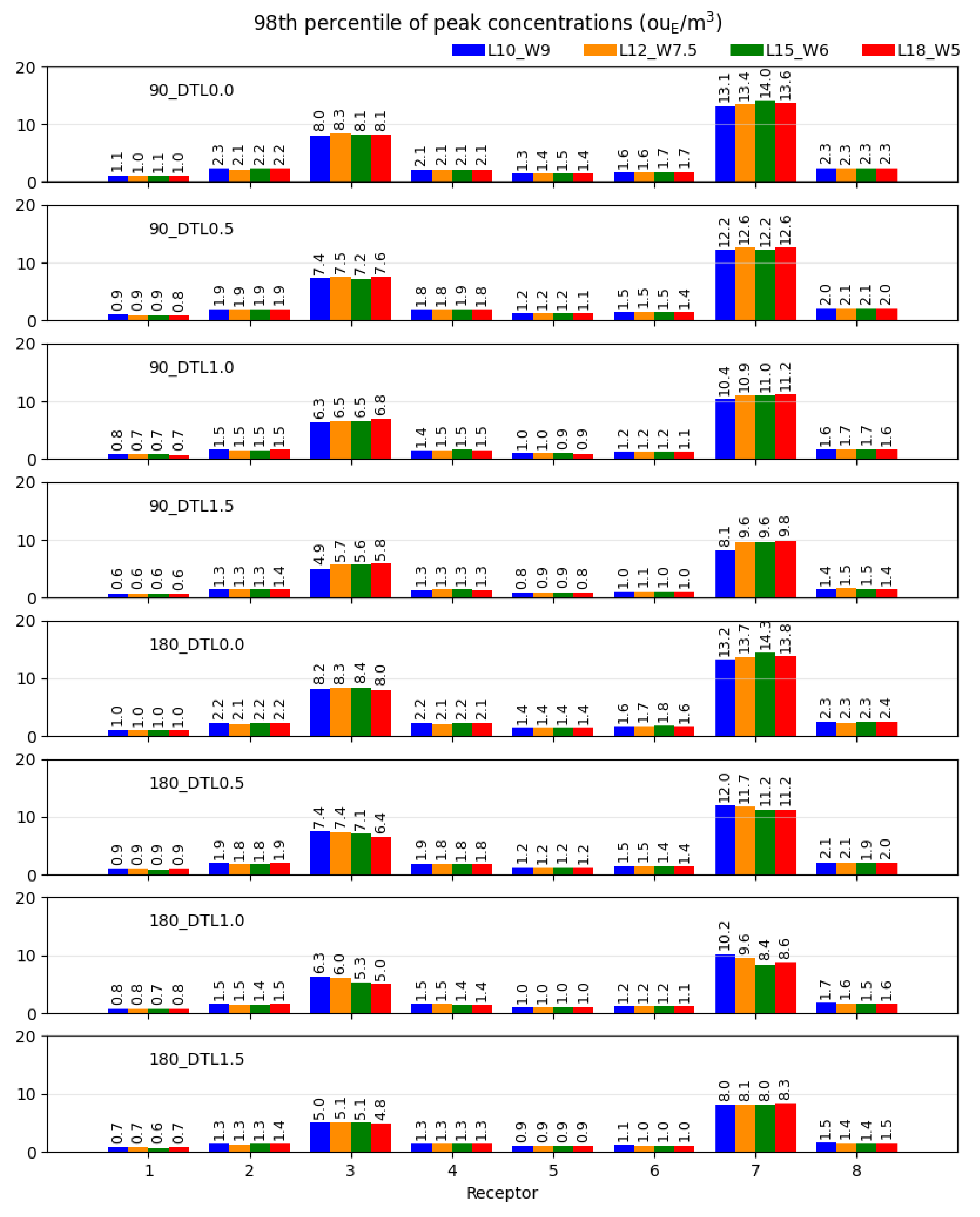
3.3. Results at Discrete Receptors

A postprocessor of LAPMOD (LAPOST) was used to analyze the output time series and characterize the odor nuisance at the discrete receptors. The 98th percentiles of the peak concentrations were extracted and are represented in Figure 14.

As explained before, the discrete receptors are placed on two rings centered on the common centroid of the tanks. Receptors R1–R8 are placed on the first ring with a radius of 500 m, while receptors R9–R16 are placed on the second ring with radius 1000 m. They are shown in Figure 10, Figure 11, Figure 12 and Figure 13. In the following, we consider only the eight inner receptors (i.e., those on the 500 m ring), which are the most impacted.

The maximum peak concentrations referring to a single hour within the whole simulation year were also extracted. However, the interpretation of those values is not simple because they depend on a combination of unfavorable meteorological conditions, both for emissions and for atmospheric dispersion. For this reason, the chart with maximum concentrations is not reported.

The 98th percentile of peak concentrations (Figure 14) shows that the maximum value was observed at R7 for all the emission scenarios; however, the maximum peak concentration was always predicted at R3 (result not shown). This result is not unexpected considering the wind rose reported in Figure 7, which shows that winds blowing from the east were more frequent than those blowing from west (i.e., 23.4% blowing from the interval 75–105 degrees, and 15.3% blowing from the interval 255–285 degrees).

Excluding tank shape factor 1.11 (i.e., L10_W9), for a fixed DTL value, concentrations at receptors 3 and 7, aligned with the longest size of the tank, were higher for the 90-degree tanks than for 180-degree tanks. This effect could be imputable to the fact that, easterly or westerly winds, which are the most frequent for the situation examined (Figure 7), are more efficient in collecting a large part of computational particles from the emitting surface and transporting them toward receptors 3 and 7 when the tank had a 90-degree orientation compared with when the tank had a 180-degree orientation. For similar reasons, the opposite was observed for receptors 1 and 5.

Figure 14 also shows different relative variations of the 98th percentile values with DTL as a function of the tank shape factor and orientation. For example, looking only at R7, considering tank L10_W9 (L/W = 1.11), when the orientation is 90 degrees, the relative variations of the 98th percentile values with respect to DTL = 0.0 m are −7.3% (DTL = 0.5 m), −20.8% (DTL = 1.0 m) and −38.0% (DTL = 1.5 m), and when the orientation is 180 degrees, the relative variations with respect to DTL = 0.0 m are −9.5% (DTL = 0.5 m), −22.9% (DTL = 1.0 m) and −39.2% (DTL = 1.5 m).

For the shape factor close to 1, the relative variations are therefore similar for both the orientations. On the contrary, if tank L18_W5 (L/W = 3.6) is considered, when the orientation is 90 degrees, the relative variations of the 98^th percentile values with respect to DTL = 0.0 m are −7.4% (DTL = 0.5 m), −17.7% (DTL = 1.0 m) and −37.5% (DTL = 1.5 m), and when the orientation is 180 degrees, the relative variations with respect to DTL = 0.0 m are −18.7% (DTL = 0.5 m), −37.5% (DTL = 1.0 m) and −40.0% (DTL = 1.5 m). Therefore, for a tank shape factor significantly different from 1, the relative variations for the same DTL value are very different as a function of the tank orientation.

3.4. Evaluation of Uncertainties

The equations used for estimating odor emissions are based on some constants that should be determined starting from the experimental results. Specifically, those constants are:

• The proportionality factor (k = 3) between the DTL and the distance of the impingement point from the leading edge, or the distance from the separation point and the trailing edge of the cavity, used in Equation (6).
• The roughness length (z₀ = 0.01 m) used in Equation (5) for determining the flow velocity close to the emitting surface.
• The height (h₀ = 0.1 m) above the odor-emitting surface at which the wind speed is evaluated, Equation (5).
• The correction factor (μ = 0.8) used in Equation (5) for determining the flow velocity close to the emitting surface.

The results obtained in this work depend on the values used for the above parameters. In order to estimate how the results would change if other values would be selected, a bootstrap procedure was applied. For simplicity, a wind of 1 m/s at the top of the tank was considered, blowing from the east (90 degrees). Different intervals of existence were assumed for the four parameters: (0.005 and 0.015 m) for z₀, (0.05 and 0.15 m) for h₀, (2.5 and 3.5) for k and (0.7 and 0.9) for μ.

Since it is not possible to assign an a priori distribution to the values, it was assumed that each value has the same probability within its interval. A Perl program was developed to randomly extract a value of each parameter and then calculate the odor emission. For each tank configuration, defined by the length, width, orientation and DTL, the procedure was run 2000 times. The statistics calculated at the end of this procedure are summarized in

Table 9. The range of variation of odor emissions (ouE/s) with the bootstrap procedure and as calculated with k = 3, z₀ = 0.01 m, h₀ = 0.1 m and μ = 0.8.

Tank	Or. (degrees)	DTL (m)	Mean (ouE/s)	Median (ouE/s)	Min (ouE/s)	Max (ouE/s)	StdDev (ouE/s)	Calculated (ouE/s)
L10_W9	90	0.5	41,691	41,730	39,328	43,251	684	41,767
L10_W9	90	1.0	36,288	36,415	31,091	39,967	1528	36,429
L10_W9	90	1.5	27,370	27,604	20,275	33,146	2388	29,891
L10_W9	180	0.5	41,258	41,315	38,950	43,141	763	41,326
L10_W9	180	1.0	35,070	35,209	28,745	39,154	1777	35,273
L10_W9	180	1.5	27,352	27,557	20,467	32,972	2364	27,610
L12_W7.5	90	0.5	42,396	42,438	40,587	43,739	556	42,418
L12_W7.5	90	1.0	38,010	38,108	34,226	40,998	1202	38,099
L12_W7.5	90	1.5	32,844	32,982	25,411	37,563	2047	33,017
L12_W7.5	180	0.5	40,336	40,403	37,131	42,602	946	40,432
L12_W7.5	180	1.0	32,633	32,865	24,711	37,868	2271	32,837
L12_W7.5	180	1.5	27,270	27,388	20,250	32,841	2293	27,610
L15_W6	90	0.5	43,003	43,035	41,594	44,107	448	43,060
L15_W6	90	1.0	39,647	39,715	36,613	41,875	915	39,698
L15_W6	90	1.5	35,756	35,837	30,559	39,342	1506	35,872
L15_W6	180	0.5	38,941	39,052	34,346	41,877	1224	39,051
L15_W6	180	1.0	28,550	28,787	21,321	34,182	2421	28,800
L15_W6	180	1.5	27,469	27,700	20,323	32,682	2355	27,610
L18_W5	90	0.5	43,447	43,470	42,238	44,396	370	43,483
L18_W5	90	1.0	40,677	40,738	38,233	42,544	743	40,729
L18_W5	90	1.5	37,590	37,654	33,897	40,379	1173	37,656
L18_W5	180	0.5	37,513	37,639	32,277	41,190	1498	37,620
L18_W5	180	1.0	28,509	28,653	21,226	34,121	2468	28,800
L18_W5	180	1.5	27,380	27,633	20,473	32,808	2362	27,610

.

The mean and the median values obtained with the bootstrap procedure are similar to those calculated with k = 3, z₀ = 0.01 m, h₀ = 0.1 m and μ = 0.8 (the values used in this work), as reported in the rightmost column of Table 9. The calculated value is always within the interval determined by the mean plus or minus a standard deviation. For each tank, the standard deviation (i.e., the uncertainty) increases with the DTL. This is likely due to the fact that, when the DTL is small, the area characterized by free flow is large (Figure 1, center), and over this area, there are no constants involved in determining the flow, since it is the external one. On the contrary, when the DTL increases, the four parameters play a role.

4. Conclusions

This paper presents a heuristic approach for estimating odor emissions from rectangular open-roof tanks as a function of the wind direction, wind speed, tank orientation, tank shape factor and vertical position of the emitting surface within the tank.

The contributions of other authors willing to apply CFD modeling and field experiments to verify the approach and, eventually, to improve it, is desirable. A reliable expression defining the ventilation of the emitting surface (i.e., the surface-average wind speed) as a function of the DTL and wind speed at the top of the tank is of particular importance. The need for a surface-averaged wind speed is important because–depending on the DTL–there could be portions of the emitting surface over which the wind speed might be high, and other parts where it could be practically absent.

Of course, the quantitative results reported in this work may differ from results where the methodology is applied for a different meteorology or a different source configuration. However, the results illustrated in this paper show the importance of the tank orientation and the DTL on the separation distances. If the effects of the tank orientation on odor emission are confirmed–with the proposed equation or others–the design of plants containing such sources should consider a detailed wind data analysis, in a similar way as is done for designing airport runways (e.g., [39]).

The distance of the odor-emitting surface from the tank top (DTL) may vary over time due to plant operations. The time variation of the DTL should be considered when conducting odor-impact-assessment studies.

The proposed equations are applicable to open-roof circular tanks as well, even though, for those tanks, only the effect of the distance between the tank top and emitting surface (DTL) will be present.

References

1. DEQ Nuisance Odor Report. State of Oregon. Department of Environmental Quality, 24 March 2014. Available online: https://www.oregon.gov/deq/FilterDocs/NuisanceOdorReport.pdf (accessed on 11 January 2022).
2. Aatamila, M.; Verkasalo, P.K.; Korhonen, M.J.; Suominen, A.L.; Hirvonen, M.-R.; Viluksela, M.K.; Nevalainen, A. Odour annoyance and physical symptoms among residents living near waste treatment centres. Environ. Res. 2011, 111, 164–170. [Google Scholar] [CrossRef] [PubMed]
3. Invernizzi, M.; Capelli, L.; Sironi, S. Proposal of Odor Nuisance Index as Urban Planning Tool. Chem. Senses 2017, 42, 105–110. [Google Scholar] [CrossRef] [Green Version]
4. Guadalupe-Fernandez, V.; De Sario, M.; Vecchi, S.; Bauleo, L.; Michelozzi, P.; Davoli, M.; Ancona, C. Industrial odour pollution and human health: A systematic review and meta-analysis. Environ. Heal. 2021, 20, 1–21. [Google Scholar] [CrossRef] [PubMed]
5. Brancher, M.; Hieden, A.; Baumann-Stanzer, K.; Schauberger, G.; Piringer, M. Performance evaluation of approaches to predict sub-hourly peak odour concentrations. Atmos. Environ. X 2020, 7, 100076. [Google Scholar] [CrossRef]
6. Barclay, J.; Diaz, C.; Galvin, G.; Bellasio, R.; Tinarelli, G.; Díaz-Robles, L.A.; Schauberger, G.; Capelli, L. New International Handbook on the Assessment of Odour Exposure Using Dispersion Modelling. Chem. Eng. Trans. 2021, 85, 175–180. [Google Scholar]
7. Carrera-Chapela, F.; Donoso-Bravo, A.; Souto, J.A.; Ruiz-Filippi, G. Modeling the Odor Generation in WWTP: An Integrated Approach Review. Water Air Soil Pollut. 2014, 225, 1932. [Google Scholar] [CrossRef] [Green Version]
8. Ravina, M.; Bruzzese, S.; Panepinto, D.; Zanetti, M. Analysis of Separation Distances under Varying Odour Emission Rates and Meteorology: A WWTP Case Study. Atmosphere 2020, 11, 962. [Google Scholar] [CrossRef]
9. Martínez-Solano, F.J.; Iglesias Rey, P.L.; Gualtieri, C.; López-Jiménez, P.A. Modelling flow and concentration field in a 3D rectangular water tank. In Proceedings of the 2010 International Congress on Environmental Modelling and Software, Ottawa, ON, Canada, 5–8 July 2010. [Google Scholar]
10. Jing, W.; Feng, H.; Cheng, X. Dynamic Responses of Liquid Storage Tanks Caused by Wind and Earthquake in Special Environment. Appl. Sci. 2019, 9, 2376. [Google Scholar] [CrossRef] [Green Version]
11. Sun, X.; Li, W.; Huang, Q.; Zhang, J.; Sun, C. Large eddy simulations of wind loads on an external floating-roof tank. Eng. Appl. Comput. Fluid Mech. 2020, 14, 422–435. [Google Scholar] [CrossRef]
12. Invernizzi, M.; Sironi, S. Odour Emission Rate Estimation Methods for Hydrocarbon Storage Tanks. Chem. Eng. Trans. 2020, 82, 67–72. [Google Scholar]
13. UE-EPA. AP-42: Compilation of Air Emissions Factors; US-EPA: Research Triangle Park, NC, USA, 2020. Available online: https://www.epa.gov/air-emissions-factors-and-quantification/ap-42-compilation-air-emissions-factors (accessed on 19 February 2022).
14. TANKS Emissions Estimation Software, Version 4.09D. Available online: https://www3.epa.gov/ttnchie1/software/tanks/ (accessed on 19 February 2022).
15. Invernizzi, M.; Ilare, J.; Capelli, L.; Sironi, S. Proposal of a Method for Evaluating Odour Emissions from Refinery Storage Tanks. Chem. Eng. Trans. 2018, 68, 49–54. [Google Scholar]
16. Rong, L.; Nielsen, P.V.; Zhang, G. Experimental and Numerical Study on Effects of Airflow and Aqueous Ammonium Solution Temperature on Ammonia Mass Transfer Coefficient. J. Air Waste Manag. Assoc. 2010, 60, 419–428. [Google Scholar] [CrossRef] [PubMed] [Green Version]
17. Cook, N. The Deaves and Harris ABL model applied to heterogeneous terrain. J. Wind Eng. Ind. Aerodyn. 1997, 66, 197–214. [Google Scholar] [CrossRef]
18. Liu, Q.; Bundy, D.S.; Hoff, S.J. A study on the air flow and odor emission rate from a simplified open manure storage tank. Trans. ASAE 1995, 38, 1881–1886. [Google Scholar] [CrossRef]
19. Bellasio, R.; Bianconi, R.; Mosca, S.; Zannetti, P. Formulation of the Lagrangian particle model LAPMOD and its evaluation against Kincaid SF6 and SO2 datasets. Atmos. Environ. 2017, 163, 87–98. [Google Scholar] [CrossRef]
20. Bellasio, R.; Bianconi, R.; Mosca, S.; Zannetti, P. Incorporation of Numerical Plume Rise Algorithms in the Lagrangian Particle Model LAPMOD and Validation against the Indianapolis and Kincaid Datasets. Atmosphere 2018, 9, 404. [Google Scholar] [CrossRef] [Green Version]
21. Region Lombardy. D.g.r. 15 Febbraio 2012–n. IX/3018. Determinazioni Generali in Merito Alla Caratterizzazione Delle Emissioni Gassose in Atmosfera Derivanti da Attività a Forte Impatto Odorigeno; Region Lombardy: Milan, Italy, 2012. (In Italian) [Google Scholar]
22. Jiang, K.; Kaye, R. Comparison study on portable wind tunnel system and isolation chamber for determination of VOCs from areal sources. Water Sci. Technol. 1996, 34, 583–589. [Google Scholar] [CrossRef]
23. Scire, J.S.; Robe, F.R.; Fernau, M.E.; Yamartino, R.J. A User’s Guide for the CALMET Meteorological Model (Version 5.0); Earth Tech Inc.: Concord, MA, USA, January 2000; Available online: http://www.src.com/calpuff/download/CALMET_UsersGuide.pdf (accessed on 19 February 2022).
24. Arya, S.P. Air Pollution Meteorology and Dispersion; Oxford University Press: Oxford, UK, 1999. [Google Scholar]
25. EPA. User’s Guide for the Industrial Source Complex (ISC3) Dispersion Model; Description of Model Algorithms; Report EPA-454/B-95-003b; US-EPA: Research Triangle Park, NC, USA, 1995; Volume II.
26. Soulhac, L.; Perkins, R.J.; Salizzoni, P. Flow in a Street Canyon for any External Wind Direction. Bound.-Layer Meteorol. 2007, 126, 365–388. [Google Scholar] [CrossRef]
27. Hotchkiss, R.S.; Harlow, F.H. Air Pollution Transport in Street Canyons; EPA-R4-73-029; US-EPA: Research Triangle Park, NC, USA, 1973.
28. Yamartino, R.J.; Wiegand, G. Development and evaluation of simple models for the flow, turbulence and pollutant concentration fields within an urban street canyon. Atmos. Environ. 1986, 20, 2137–2156. [Google Scholar] [CrossRef]
29. Berkowicz, R.; Hertel, O.; Larsen, S.E.; Sørensen, N.N.; Nielsen, M. Modelling Traffic Pollution in Streets; National Environmental Research Institute: Roskilde, Denmark, 1997. [Google Scholar]
30. Huang, L.; Zhao, K.; Liang, J.; Kopiev, V.; Belyaev, I.; Zhang, T. A Numerical Study of the Wind Speed Effect on the Flow and Acoustic Characteristics of the Minor Cavity Structures in a Two-Wheel Landing Gear. Appl. Sci. 2021, 11, 11235. [Google Scholar] [CrossRef]
31. Crook, S.D.; Lau, T.C.W.; Kelso, R.M. Three-dimensional flow within shallow, narrow cavities. J. Fluid Mech. 2013, 735, 587–612. [Google Scholar] [CrossRef]
32. Ashcroft, G.; Zhang, X. Vortical structures over rectangular cavities at low speed. Phys. Fluids 2005, 17, 015104. [Google Scholar] [CrossRef]
33. Chang, J.C.; Hanna, S.R. Air quality model performance evaluation. Arch. Meteorol. Geophys. Bioclimatol. Ser. B 2004, 87, 167–196. [Google Scholar] [CrossRef]
34. Haq, A.U.; Nadeem, Q.; Farooq, A.; Irfan, N.; Ahmad, M.; Ali, M.R. Assessment of Lagrangian particle dispersion model “LAPMOD” through short range field tracer test in complex terrain. J. Environ. Radioact. 2019, 205-206, 34–41. [Google Scholar] [CrossRef]
35. Invernizzi, M.; Brancher, M.; Sironi, S.; Capelli, L.; Piringer, M.; Schauberger, G. Odour impact assessment by considering short-term ambient concentrations: A multi-model and two-site comparison. Environ. Int. 2020, 144, 105990. [Google Scholar] [CrossRef] [PubMed]
36. Vitali, L.; Monforti, F.; Bellasio, R.; Bianconi, R.; Sachero, V.; Mosca, S.; Zanini, G. Validation of a Lagrangian dispersion model implementing different kernel methods for density reconstruction. Atmos. Environ. 2006, 40, 8020–8033. [Google Scholar] [CrossRef]
37. Mylne, K.R.; Mason, P.J. Concentration fluctuation measurements in a dispersing at a range up to 1000 m. Q. J. R. Meteorol. Soc. 1991, 117, 177–206. [Google Scholar] [CrossRef]
38. Weather Research and Forecasting Model. Available online: https://www.mmm.ucar.edu/weather-research-and-forecasting-model (accessed on 11 January 2022).
39. Bellasio, R. Analysis of wind data for airport runway design. J. Airl. Airpt. Manag. 2014, 4, 97–116. [Google Scholar] [CrossRef]
Figure 1. Schematization of the flow types within a cavity.
Atmosphere 13 00367 g001
Figure 2. Simple schematization of the rectangular tank. The gray surface represents the emitting surface.
Atmosphere 13 00367 g002
Figure 3. Path calculation when wind crosses the longest size of the tank (L).
Atmosphere 13 00367 g003
Figure 4. Path calculation when wind crosses the shortest size of the tank (W).
Atmosphere 13 00367 g004
Figure 5. Definition of the limiting angles. Top view of the tank.
Atmosphere 13 00367 g005
Figure 6. Wind path approximation. P is represented by the dashed black lines, while Pa is represented by the blue dashed lines. Top: the wind vector enters and exits through L. Bottom: the wind vector enters and exits through W.
Atmosphere 13 00367 g006
Figure 7. Wind rose of the computational grid containing the source.
Atmosphere 13 00367 g007
Figure 8. Annual emissions of odor (109 ouE/year) for the different tanks and scenarios. (A): tank L10_W9, shape factor 1.11. (B): tank L12_W7.5, shape factor 1.60. (C): tank L15_W6, shape factor 2.50. (D): tank L18_W5, shape factor 3.60.
Atmosphere 13 00367 g008
Figure 9. Box and whiskers plot of the OERs (ouE/s) for the different tanks and scenarios. The green circle represents the mean value, while the red segment represents the median value. The mean and median values are also numerically reported in the upper part of the figure. (A): tank L10_W9, shape factor 1.11. (B): tank L12_W7.5, shape factor 1.60. (C): tank L15_W6, shape factor 2.50. (D): tank L18_W5, shape factor 3.60.
Atmosphere 13 00367 g009
Figure 10. Tank L10_W9. Separation distances calculated for the base case (top row) and as a function of the tank orientation and DTL of 0.5 m (second row), 1.0 m (third row) and 1.5 m (bottom row). Concentration thresholds are 1 ouE/m3 (left column), 3 ouE/m3 (central column) and 5 ouE/m3 (right column). The dark green circle represents the centroid of the sources, while the black crosses represent the discrete receptors. (A): DTL = 0.0 m, CT = 1 ouE/m3. (B): DTL = 0.0 m, CT = 3 ouE/m3. (C): DTL = 0.0 m, CT = 5 ouE/m3. (D): DTL = 0.5 m, CT = 1 ouE/m3. (E): DTL = 0.5 m, CT = 3 ouE/m3. (F): DTL = 0.5 m, CT = 5 ouE/m3. (G): DTL = 1.0 m, CT = 1 ouE/m3. (H): DTL = 1.0 m, CT = 3 ouE/m3. (I): DTL = 1.0 m, CT = 5 ouE/m3. (J): DTL = 1.5 m, CT = 1 ouE/m3. (K): DTL = 1.5 m, CT = 3 ouE/m3. (L): DTL = 1.5 m, CT = 5 ouE/m3.
Atmosphere 13 00367 g010
Figure 11. Tank L12_W7.5. Separation distances calculated for the base case (top row) and as a function of the tank orientation and DTL of 0.5 m (second row), 1.0 m (third row) and 1.5 m (bottom row). Concentration thresholds are 1 ouE/m3 (left column), 3 ouE/m3 (central column) and 5 ouE/m3 (right column). The dark green circle represents the centroid of the sources, while the black crosses represent the discrete receptors. (A): DTL = 0.0 m, CT = 1 ouE/m3. (B): DTL = 0.0 m, CT = 3 ouE/m3. (C): DTL = 0.0 m, CT = 5 ouE/m3. (D): DTL = 0.5 m, CT = 1 ouE/m3. (E): DTL = 0.5 m, CT = 3 ouE/m3. (F): DTL = 0.5 m, CT = 5 ouE/m3. (G): DTL = 1.0 m, CT = 1 ouE/m3. (H): DTL = 1.0 m, CT = 3 ouE/m3. (I): DTL = 1.0 m, CT = 5 ouE/m3. (J): DTL = 1.5 m, CT = 1 ouE/m3. (K): DTL = 1.5 m, CT = 3 ouE/m3. (L): DTL = 1.5 m, CT = 5 ouE/m3.
Atmosphere 13 00367 g011
Figure 12. Tank L15_W6. Separation distances calculated for the base case (top row) and as a function of the tank orientation and DTL of 0.5 m (second row), 1.0 m (third row) and 1.5 m (bottom row). Concentration thresholds are 1 ouE/m3 (left column), 3 ouE/m3 (central column) and 5 ouE/m3 (right column). The dark green circle represents the centroid of the sources, while the black crosses represent the discrete receptors. (A): DTL = 0.0 m, CT = 1 ouE/m3. (B): DTL = 0.0 m, CT = 3 ouE/m3. (C): DTL = 0.0 m, CT = 5 ouE/m3. (D): DTL = 0.5 m, CT = 1 ouE/m3. (E): DTL = 0.5 m, CT = 3 ouE/m3. (F): DTL = 0.5 m, CT = 5 ouE/m3. (G): DTL = 1.0 m, CT = 1 ouE/m3. (H): DTL = 1.0 m, CT = 3 ouE/m3. (I): DTL = 1.0 m, CT = 5 ouE/m3. (J): DTL = 1.5 m, CT = 1 ouE/m3. (K): DTL = 1.5 m, CT = 3 ouE/m3. (L): DTL = 1.5 m, CT = 5 ouE/m3.
Atmosphere 13 00367 g012
Figure 13. Tank L18_W5. Separation distances calculated for the base case (top row) and as a function of the tank orientation and DTL of 0.5 m (second row), 1.0 m (third row) and 1.5 m (bottom row). Concentration thresholds are 1 ouE/m3 (left column), 3 ouE/m3 (central column) and 5 ouE/m3 (right column). The dark green circle represents the centroid of the sources, while the black crosses represent the discrete receptors. (A): DTL = 0.0 m, CT = 1 ouE/m3. (B): DTL = 0.0 m, CT = 3 ouE/m3. (C): DTL = 0.0 m, CT = 5 ouE/m3. (D): DTL = 0.5 m, CT = 1 ouE/m3. (E): DTL = 0.5 m, CT = 3 ouE/m3. (F): DTL = 0.5 m, CT = 5 ouE/m3. (G): DTL = 1.0 m, CT = 1 ouE/m3. (H): DTL = 1.0 m, CT = 3 ouE/m3. (I): DTL = 1.0 m, CT = 5 ouE/m3. (J): DTL = 1.5 m, CT = 1 ouE/m3. (K): DTL = 1.5 m, CT = 3 ouE/m3. (L): DTL = 1.5 m, CT = 5 ouE/m3.
Atmosphere 13 00367 g013
Figure 14. The 98th percentiles of peak concentrations (ouE/m3) at discrete receptors for the eight emission scenarios.
Atmosphere 13 00367 g014