
Valley–Mountain Circulation Associated with the Diurnal Cycle of Precipitation in the Tropical Andes (Santa River Basin, Peru)

 , ,
, ,  and
and
Abstract
1. Introduction
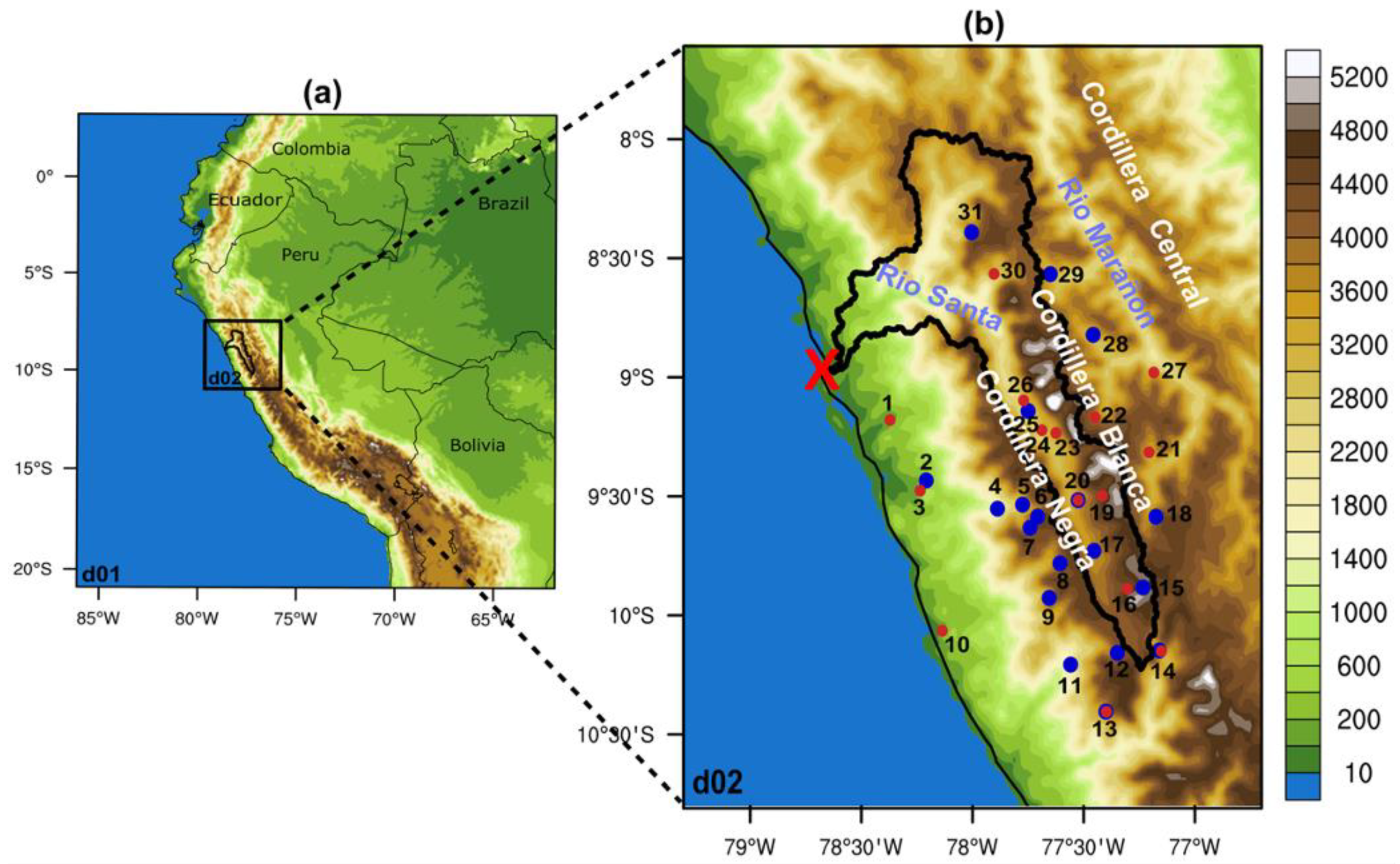
2. Main Climatic Features
3. Data and Model
3.1. In Situ Data
3.2. Precipitation Products
3.3. WRF Simulations
4. Evaluation of the Diurnal Cycle of Precipitation in the Santa River Basin
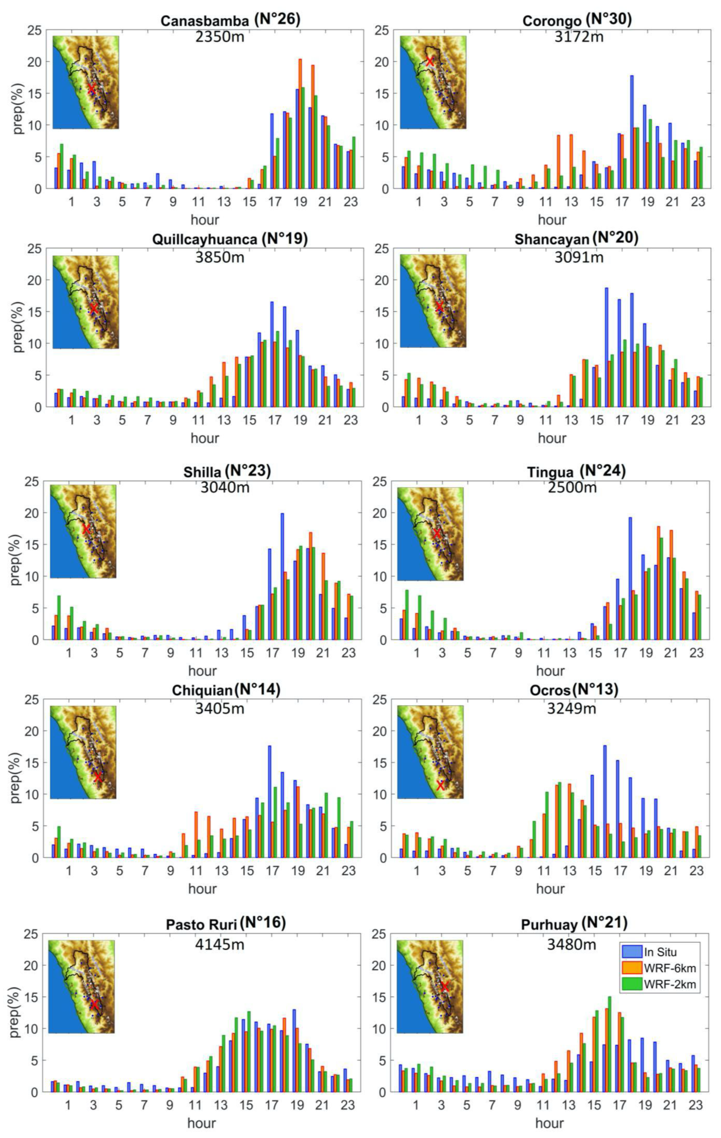
4.1. Local Scale
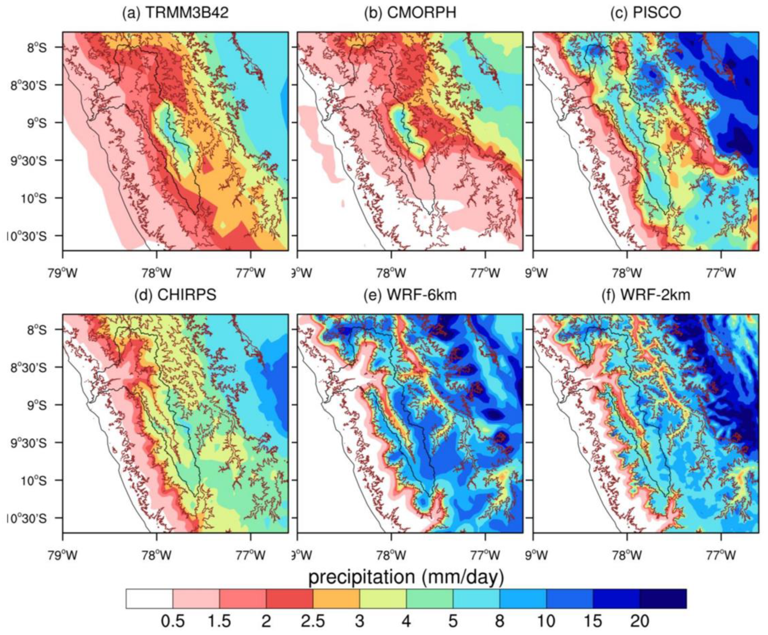
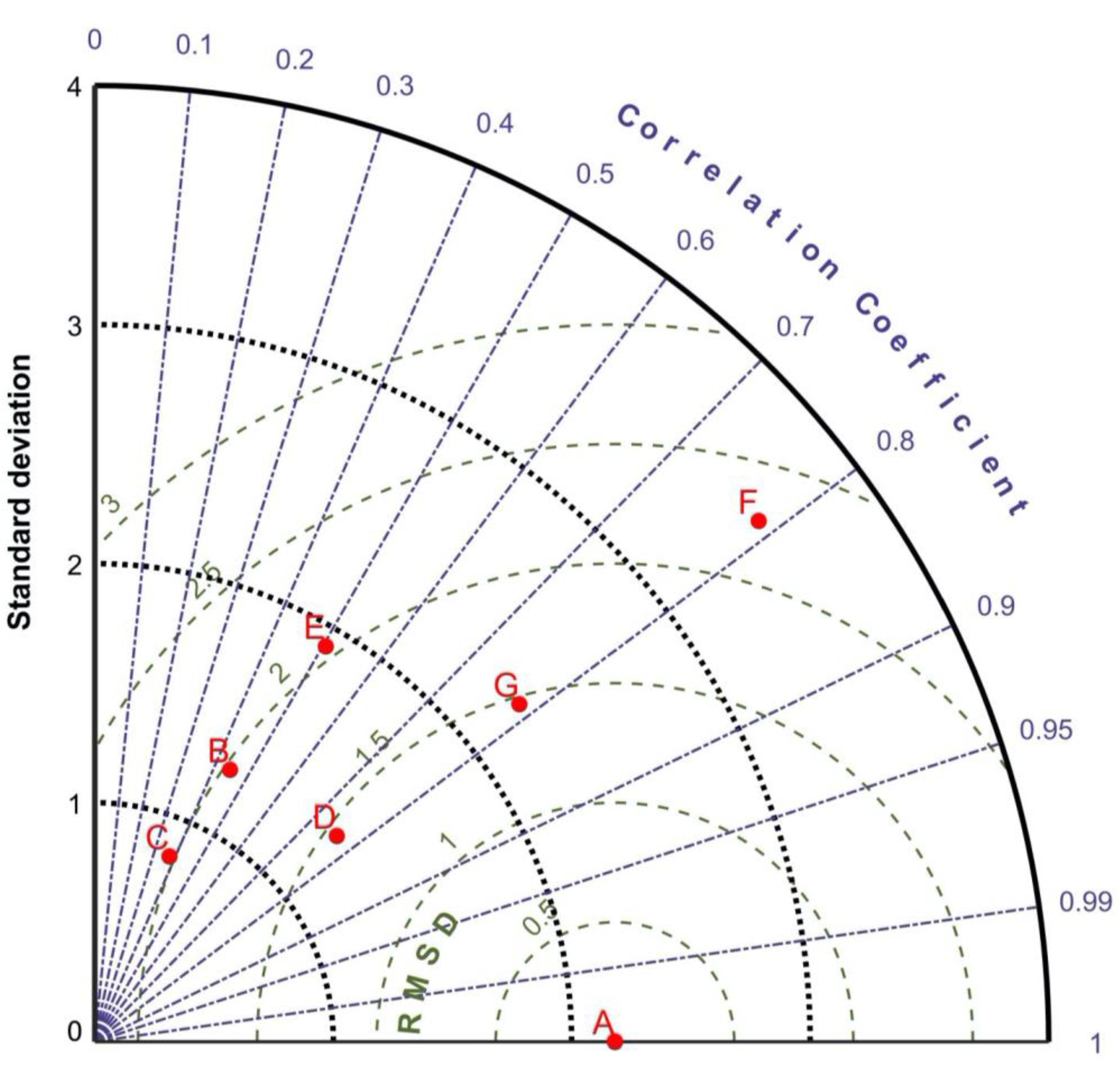
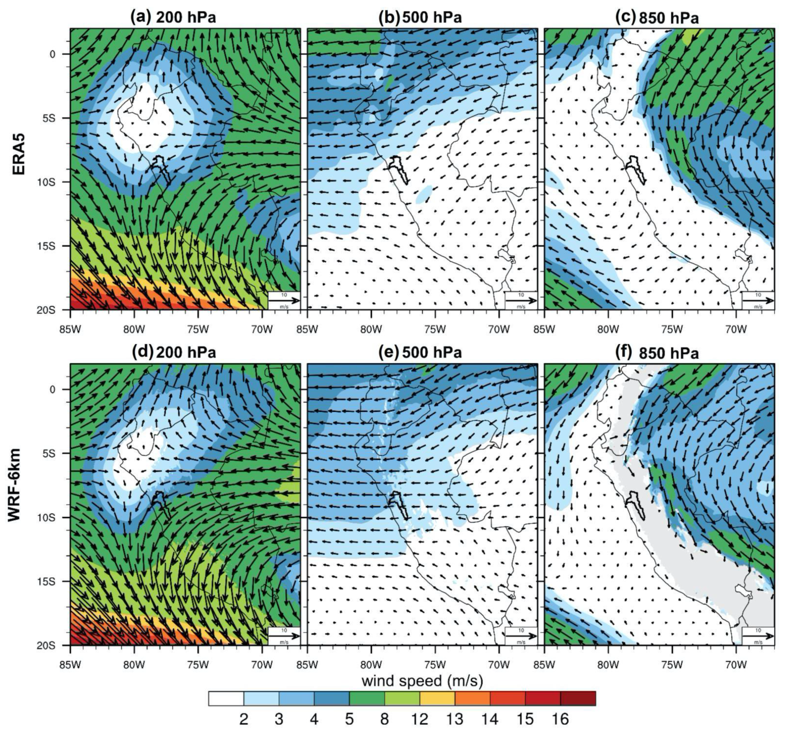
4.2. Regional Scale
5. Atmospheric Processes Associated with the Diurnal Cycle of Precipitation
5.1. Diurnal Cycle of Moisture Fluxes Related to Precipitation
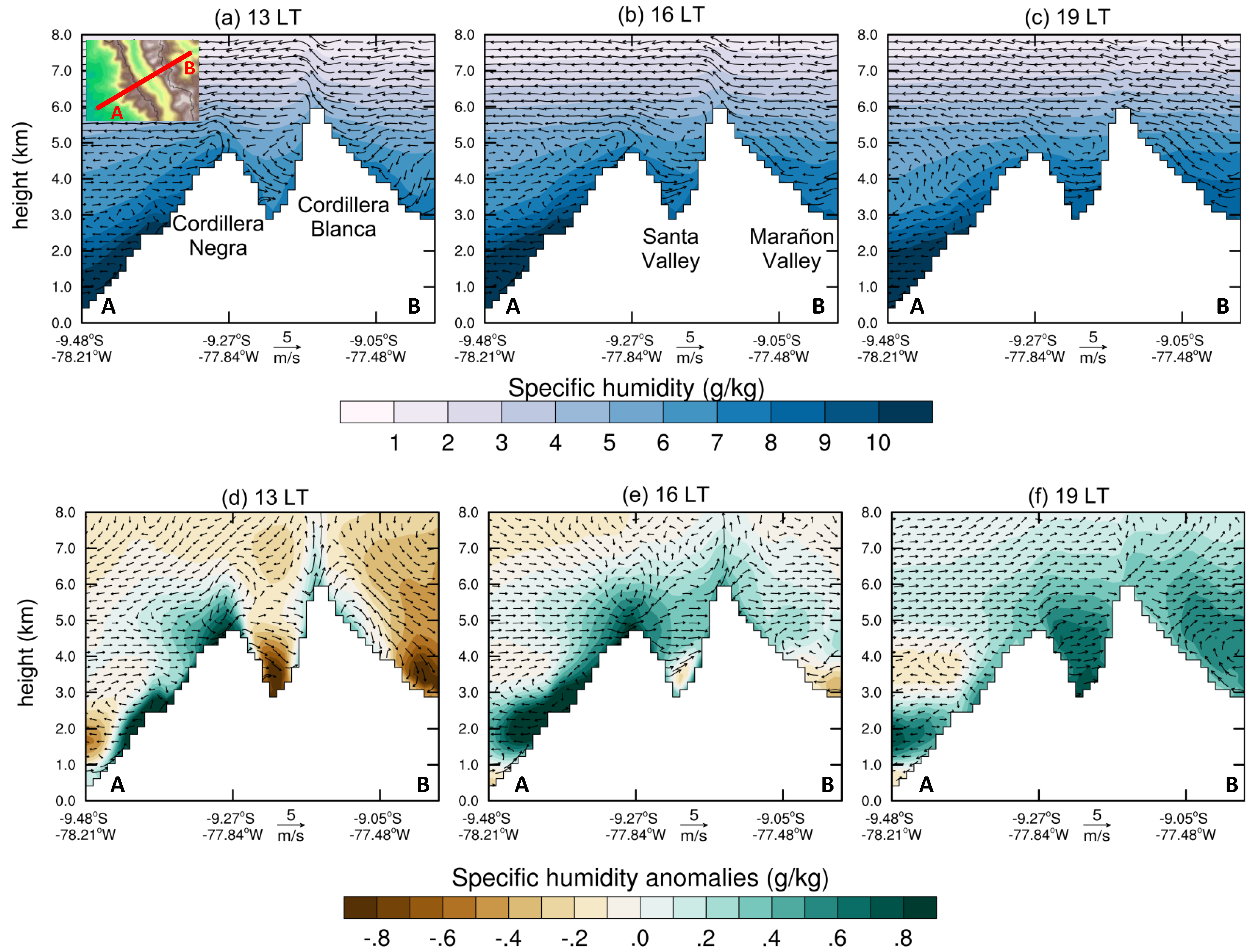
5.2. Regional and Local Atmospheric Processes Controlling the Afternoon and Early Night Precipitation
6. Summary and Conclusions
Supplementary Materials
Author Contributions
Funding
Data Availability Statement
Acknowledgments
Conflicts of Interest
References
- Zapata, M.; Arnaud, Y.; Gallaire, R. Inventario de Glaciares de La Cordillera Blanca. In Proceedings of the 13th IWRA World Water Congress, Montpellier, France, 1–4 September 2008. [Google Scholar]
- Vignon, F. Glaciares y Recursos Hídricos en el Valle Alto del Río Santa. Ph.D. Thesis, Paris Diderot University, Paris, France, 2002. [Google Scholar]
- Kaser, G.; Ames, A.; Zamora, M. Glacier Fluctuations and Climate in the Cordillera Blanca, Peru. Ann. Glaciol. 1990, 14, 136–140. [Google Scholar] [CrossRef]
- Georges, C. 20th-Century Glacier Fluctuations in the Tropical Cordillera Blanca, Peru. Arct. Antarct. Alp. Res. 2004, 36, 100–107. [Google Scholar] [CrossRef]
- Vuille, M.; Kaser, G.; Juen, I. Glacier Mass Balance Variability in the Cordillera Blanca, Peru and Its Relationship with Climate and the Large-Scale Circulation. Glob. Planet. Chang. 2008, 62, 14–28. [Google Scholar] [CrossRef]
- Condom, T.; Escobar, M.; Purkey, D.; Pouget, J.C.; Suárez, W.; Ramos, C.; Apaestegui, J.; Tacsi, A.; Gómez, J. Simulating the Implications of Glaciers’ Retreat for Water Management: A Case Study in the Rio Santa Basin, Peru. Water Int. 2012, 37, 442–459. [Google Scholar] [CrossRef]
- Junquas, C.; Takahashi, K.; Condom, T.; Espinoza, J.-C.; Chavez, S.; Sicart, J.-E.; Lebel, T. Understanding the Influence of Orography on the Precipitation Diurnal Cycle and the Associated Atmospheric Processes in the Central Andes. Clim. Dyn. 2018, 50, 3995–4017. [Google Scholar] [CrossRef]
- Mejía, F.; Douglas, M. Flow around the Andean Elbow from WRF Simulations and P-3 Aircraft Measurements during the SALLJEX. In Proceedings of the 8th International Conference on Southern Hemisphere Meteorology and Oceanography (ICSHMO), Foz de Iguaçu, Brazil, 24–28 April 2006; INPE: São José dos Campos, Brazil, 2006; pp. 795–802. [Google Scholar]
- Moya-Álvarez, A.S.; Martínez-Castro, D.; Flores, J.L.; Silva, Y. Sensitivity Study on the Influence of Parameterization Schemes in WRF_ARW Model on Short- and Medium-Range Precipitation Forecasts in the Central Andes of Peru. Adv. Meteorol. 2018, 2018, 1381092. [Google Scholar] [CrossRef]
- Ochoa-Sánchez, A.E.; Pineda Ordonez, L.E.; Crespo, P.; Willems, P. Evaluation of TRMM 3B42 Precipitation Estimates and WRF Retrospective Precipitation Simulation over the Pacific-Andean Region of Ecuador and Peru. Hydrol. Earth Syst. Sci. 2014, 18, 3179–3193. [Google Scholar] [CrossRef]
- Spiga, A.; Teitelbaum, H.; Zeitlin, V. Identification of the Sources of Inertia-Gravity Waves in the Andes Cordillera Region. Ann. Geophys. 2008, 26, 2551–2568. [Google Scholar] [CrossRef][Green Version]
- Saavedra, M.; Junquas, C.; Espinoza, J.-C.; Silva, Y. Impacts of Topography and Land Use Changes on the Air Surface Temperature and Precipitation over the Central Peruvian Andes. Atmos. Res. 2020, 234, 104711. [Google Scholar] [CrossRef]
- Mourre, L.; Condom, T.; Junquas, C.; Lebel, T.; Sicart, J.E.; Figueroa, R.; Cochachin, A. Spatio-Temporal Assessment of WRF, TRMM and in Situ Precipitation Data in a Tropical Mountain Environment (Cordillera Blanca, Peru). Hydrol. Earth Syst. Sci. 2016, 20, 125–141. [Google Scholar] [CrossRef]
- Skamarock, W.C.; Klemp, J.B.; Dudhia, J.; Gill, D.O.; Barker, D.M.; Duda, M.G.; Huang, X.-Y.; Wang, W.; Powers, J.G. A Description of the Advanced Research WRF Version 3; Technical Report NCAR/TN–475+STR; NCAR: Boulder, CO, USA, 2008; 125p. [Google Scholar]
- Garreaud, R.D. The Andes Climate and Weather. Adv. Geosci. 2009, 22, 3–11. [Google Scholar] [CrossRef]
- Houze, R.A. Orographic Effects on Precipitating Clouds. Rev. Geophys. 2012, 50, RG1001. [Google Scholar] [CrossRef]
- Garreaud, R.D. Multiscale Analysis of the Summertime Precipitation over the Central Andes. Mon. Weather Rev. 1999, 127, 901–921. [Google Scholar] [CrossRef]
- Espinoza, J.C.; Garreaud, R.; Poveda, G.; Arias, P.A.; Molina-Carpio, J.; Masiokas, M.; Viale, M.; Scaff, L. Hydroclimate of the Andes Part I: Main Climatic Features. Front. Earth Sci. 2020, 8, 64. [Google Scholar] [CrossRef]
- Chavez, S.P.; Takahashi, K. Orographic Rainfall Hot Spots in the Andes-Amazon Transition According to the TRMM Precipitation Radar and In Situ Data. J. Geophys. Res. Atmos. 2017, 122, 5870–5882. [Google Scholar] [CrossRef]
- Espinoza, J.C.; Chavez, S.; Ronchail, J.; Junquas, C.; Takahashi, K.; Lavado, W. Rainfall Hotspots over the Southern Tropical Andes: Spatial Distribution, Rainfall Intensity, and Relations with Large-Scale Atmospheric Circulation. Water Resour. Res. 2015, 51, 3459–3475. [Google Scholar] [CrossRef]
- Garreaud, R.; Vuille, M.; Clement, A.C. The Climate of the Altiplano: Observed Current Conditions and Mechanisms of Past Changes. Palaeogeogr. Palaeoclimatol. Palaeoecol. 2003, 194, 5–22. [Google Scholar] [CrossRef]
- Staal, A.; Tuinenburg, O.A.; Bosmans, J.H.C.; Holmgren, M.; van Nes, E.H.; Scheffer, M.; Zemp, D.C.; Dekker, S.C. Forest-Rainfall Cascades Buffer against Drought across the Amazon. Nat. Clim. Chang. 2018, 8, 539–543. [Google Scholar] [CrossRef]
- Ampuero, A.; Stríkis, N.M.; Apaéstegui, J.; Vuille, M.; Novello, V.F.; Espinoza, J.C.; Cruz, F.W.; Vonhof, H.; Mayta, V.C.; Martins, V.T.S.; et al. The Forest Effects on the Isotopic Composition of Rainfall in the Northwestern Amazon Basin. J. Geophys. Res. Atmos. 2020, 125, e2019JD031445. [Google Scholar] [CrossRef]
- Falvey, M.; Garreaud, R.D. Moisture Variability over the South American Altiplano during the South American Low Level Jet Experiment (SALLJEX) Observing Season. J. Geophys. Res. 2005, 110, D22105. [Google Scholar] [CrossRef]
- Romatschke, U.; Houze, R.A. Extreme Summer Convection in South America. J. Clim. 2010, 23, 3761–3791. [Google Scholar] [CrossRef]
- Enfield, D.B. Thermally Driven Wind Variability in the Planetary Boundary Layer above Lima, Peru. J. Geophys. Res. 1981, 86, 2005–2016. [Google Scholar] [CrossRef]
- Takahashi, K. Thermotidal and Land-Heating Forcing of the Diurnal Cycle of Oceanic Surface Winds in the Eastern Tropical Pacific. Geophys. Res. Lett. 2012, 39, L04805. [Google Scholar] [CrossRef]
- Trachte, K.; Seidel, J.; Figueroa, R.; Otto, M.; Bendix, J. Cross-Scale Precipitation Variability in a Semiarid Catchment Area on the Western Slopes of the Central Andes. J. Appl. Meteorol. Climatol. 2018, 57, 675–694. [Google Scholar] [CrossRef]
- Gutman, G.J.; Schwerdtfeger, W. The Role of Latent and Sensible Heat for the Development of a High Pressure System over the Subtropical Andes, in the Summer (Role of Latent Heat in Development of Anticyclone Pressure System over Subtropical Andes during Summer Months—TIROS II Radiation Data); Springer: Berlin/Heidelberg, Germany, 1965; pp. 95–124. [Google Scholar]
- Virji, H. A Preliminary Study of Summertime Tropospheric Circulation Patterns over South America Estimated from Cloud Winds. Mon. Weather Rev. 1981, 109, 599–610. [Google Scholar] [CrossRef]
- Vera, C.; Higgins, W.; Amador, J.; Ambrizzi, T.; Garreaud, R.; Gochis, D.; Gutzler, D.; Lettenmaier, D.; Marengo, J.; Mechoso, C.R.; et al. Toward a Unified View of the American Monsoon Systems. J. Clim. 2006, 19, 4977–5000. [Google Scholar] [CrossRef]
- Lenters, J.D.; Cook, K.H. Summertime Precipitation Variability over South America: Role of the Large-Scale Circulation. Mon. Weather Rev. 1999, 127, 409–431. [Google Scholar] [CrossRef]
- Figueroa, S.N.; Satyamurty, P.; Da Silva Dias, P.L. Simulations of the Summer Circulation over the South American Region with an Eta Coordinate Model. J. Atmos. Sci. 1995, 52, 1573–1584. [Google Scholar] [CrossRef]
- Aceituno, P.; Montecinos, A. Circulation Anomalies Associated with Dry and Wet Periods in the South American Altiplano. In Proceedings of the Fourth International Conference on Southern Hemisphere Meteorology, Hobart, Australia, 29 March–2 April 1993; pp. 330–331. [Google Scholar]
- Kodama, Y. Large-Scale Common Features of Subtropical Precipitation Zones (the Baiu Frontal Zone, the SPCZ, and the SACZ) Part I: Characteristics of Subtropical Frontal Zones. J. Meteorol. Soc. Jpn. Ser. II 1992, 70, 813–836. [Google Scholar] [CrossRef]
- Marengo, J.A.; Liebmann, B.; Grimm, A.M.; Misra, V.; da Silva Dias, P.L.; Cavalcanti, I.F.A.; Carvalho, L.M.V.; Berbery, E.H.; Ambrizzi, T.; Vera, C.S.; et al. Recent Developments on the South American Monsoon System. Int. J. Climatol. 2012, 32, 1–21. [Google Scholar] [CrossRef]
- Zhou, J.; Lau, K.M. Does a Monsoon Climate Exist over South America? J. Clim. 1998, 11, 1020–1040. [Google Scholar] [CrossRef]
- Liebmann, B.; Marengo, J. Interannual Variability of the Rainy Season and Rainfall in the Brazilian Amazon Basin. J. Clim. 2001, 14, 4308–4318. [Google Scholar] [CrossRef]
- Marengo, J.A.; Douglas, M.W.; Dias, P.L.S. The South American Low-level Jet East of the Andes during the 1999 LBA-TRMM and LBA-WET AMC Campaign. J. Geophys. Res. Atmos. 2002, 107, LBA-47. [Google Scholar] [CrossRef]
- Segura, H.; Espinoza, J.C.; Junquas, C.; Lebel, T.; Vuille, M.; Garreaud, R. Recent Changes in the Precipitation-Driving Processes over the Southern Tropical Andes/Western Amazon. Clim. Dyn. 2020, 54, 2613–2631. [Google Scholar] [CrossRef]
- Rodwell, M.J.; Hoskins, B.J. Subtropical Anticyclones and Summer Monsoons. J. Clim. 2001, 14, 3192–3211. [Google Scholar] [CrossRef]
- Junquas, C.; Li, L.; Vera, C.S.; Le Treut, H.; Takahashi, K. Influence of South America Orography on Summertime Precipitation in Southeastern South America. Clim. Dyn. 2016, 46, 3941–3963. [Google Scholar] [CrossRef]
- Poveda, G.; Mesa, O.J.; Salazar, L.F.; Arias, P.A.; Moreno, H.A.; Vieira, S.C.; Agudelo, P.A.; Toro, V.G.; Alvarez, J.F. The Diurnal Cycle of Precipitation in the Tropical Andes of Colombia. Mon. Weather Rev. 2005, 133, 228–240. [Google Scholar] [CrossRef]
- Ruiz-Hernández, J.C.; Condom, T.; Espinoza, J.C.; Junquas, C.; Ribstein, P.; Villacis, M.; Lemoine, N.; Sicart, J.E.; Rabatel, A.; Campozano, L.; et al. Spatial Variability of Diurnal to Seasonal Cycles of Precipitation from a High-Altitude Equatorial Andean Valley to the Amazon Basin. J. Hydrol. Reg. Stud. 2021, 38, 100924. [Google Scholar] [CrossRef]
- Campozano, L.; Célleri, R.; Trachte, K.; Bendix, J.; Samaniego, E. Rainfall and Cloud Dynamics in the Andes: A Southern Ecuador Case Study. Adv. Meteorol. 2016, 2016, 3192765. [Google Scholar] [CrossRef]
- Egger, J.; Blacutt, L.; Ghezzi, F.; Heinrich, R.; Kolb, P.; Lämmlein, S.; Leeb, M.; Mayer, S.; Palenque, E.; Reuder, J.; et al. Diurnal Circulation of the Bolivian Altiplano. Part I: Observations. Mon. Weather Rev. 2005, 133, 911–924. [Google Scholar] [CrossRef][Green Version]
- Giovannettone, J.P.; Barros, A.P. Probing Regional Orographic Controls of Precipitation and Cloudiness in the Central Andes Using Satellite Data. J. Hydrometeorol. 2009, 10, 167–182. [Google Scholar] [CrossRef]
- Reuder, J.; Egger, J. Diurnal Circulation of the South American Altiplano: Observations in a Valley and at a Pass. Tellus A Dyn. Meteorol. Oceanogr. 2006, 58, 254–262. [Google Scholar] [CrossRef]
- Trachte, K.; Rollenbeck, R.; Bendix, J. Nocturnal Convective Cloud Formation under Clear-Sky Conditions at the Eastern Andes of South Ecuador. J. Geophys. Res. 2010, 115, 24203. [Google Scholar] [CrossRef]
- Trachte, K.; Nauss, T.; Bendix, J. The Impact of Different Terrain Configurations on the Formation and Dynamics of Katabatic Flows: Idealised Case Studies. Bound.-Layer Meteorol. 2010, 134, 307–325. [Google Scholar] [CrossRef]
- Funk, C.; Peterson, P.; Landsfeld, M.; Pedreros, D.; Verdin, J.; Shukla, S.; Husak, G.; Rowland, J.; Harrison, L.; Hoell, A.; et al. The Climate Hazards Infrared Precipitation with Stations—A New Environmental Record for Monitoring Extremes. Sci. Data 2015, 2, 150066. [Google Scholar] [CrossRef] [PubMed]
- Huffman, G.J.; Adler, R.F.; Bolvin, D.T.; Gu, G.; Nelkin, E.J.; Bowman, K.P.; Hong, Y.; Stocker, E.F.; Wolff, D.B. The TRMM Multisatellite Precipitation Analysis (TMPA): Quasi-Global, Multiyear, Combined-Sensor Precipitation Estimates at Fine Scales. J. Hydrometeorol. 2007, 8, 38–55. [Google Scholar] [CrossRef]
- Kummerow, C.; Simpson, J.; Thiele, O.; Barnes, W.; Chang, A.T.C.; Stocker, E. The Status of the Tropical Rainfall Measuring Mission (TRMM) after Two Years in Orbit. J. Appl. Meteorol. 2000, 39, 1965–1982. [Google Scholar] [CrossRef]
- Joyce, R.J.; Janowiak, J.E.; Arkin, P.A.; Xie, P. CMORPH: A Method That Produces Global Precipitation Estimates from Passive Microwave and Infrared Data at High Spatial and Temporal Resolution. J. Hydrometeorol. 2004, 5, 487–503. [Google Scholar] [CrossRef]
- Rosales, A.J.G. Valley-Mountain Circulation Associated with Precipitation Formation in the Tropical Andes (Rio Santa Basin). Master’s Thesis, Universidade de São Paulo, São Paulo, Brazil, 2019. [Google Scholar]
- Betts, A.K. A New Convective Adjustment Scheme. Part I: Observational and Theoretical Basis. Q. J. R. Meteorol. Soc. 1986, 112, 677–691. [Google Scholar] [CrossRef]
- Betts, A.K.; Miller, M.J. A New Convective Adjustment Scheme. Part II: Single Column Tests Using GATE Wave, BOMEX, ATEX and Arctic Air-Mass Data Sets. Q. J. R. Meteorol. Soc. 1986, 112, 693–709. [Google Scholar] [CrossRef]
- Janjić, Z.I. The Step-Mountain Eta Coordinate Model: Further Developments of the Convection, Viscous Sublayer, and Turbulence Closure Schemes. Mon. Weather Rev. 1994, 122, 927–945. [Google Scholar] [CrossRef]
- Tao, W.-K.; Simpson, J.; McCumber, M. An Ice-Water Saturation Adjustment. Mon. Weather Rev. 1989, 117, 231–235. [Google Scholar] [CrossRef]
- Nakanishi, M.; Niino, H. An Improved Mellor-Yamada Level-3 Model: Its Numerical Stability and Application to a Regional Prediction of Advection Fog. Bound.-Layer Meteorol. 2006, 119, 397–407. [Google Scholar] [CrossRef]
- Niu, G.-Y.; Yang, Z.-L.; Mitchell, K.E.; Chen, F.; Ek, M.B.; Barlage, M.; Kumar, A.; Manning, K.; Niyogi, D.; Rosero, E.; et al. The Community Noah Land Surface Model with Multiparameterization Options (Noah-MP): 1. Model Description and Evaluation with Local-Scale Measurements. J. Geophys. Res. Atmos. 2011, 116, D12109. [Google Scholar] [CrossRef]
- Yang, Z.; Niu, G.; Mitchell, K.E.; Chen, F.; Ek, M.B.; Barlage, M.; Longuevergne, L.; Manning, K.; Niyogi, D.; Tewari, M.; et al. The Community Noah Land Surface Model with Multiparameterization Options (Noah-MP): 2. Evaluation over Global River Basins. J. Geophys. Res. Atmos. 2011, 116, D12110. [Google Scholar] [CrossRef]
- Junquas, C.; Heredia, M.B.; Condom, T.; Ruiz-Hernández, J.C.; Campozano, L.; Dudhia, J.; Espinoza, J.C.; Menegoz, M.; Rabatel, A.; Sicart, J.E. Regional Climate Modeling of the Diurnal Cycle of Precipitation and Associated Atmospheric Circulation Patterns over an Andean Glacier Region (Antisana, Ecuador). Clim. Dyn. 2022. [Google Scholar] [CrossRef]
- Nakanishi, M.; Niino, H. An improved Mellor-Yamada level-3 model with condensation physics: Its design and verification. Bound.-Layer Meteorol. 2004, 112, 1–31. [Google Scholar] [CrossRef]
- Iacono, M.J.; Delamere, J.S.; Mlawer, E.J.; Shephard, M.W.; Clough, S.A.; Collins, W.D. Radiative Forcing by Long-Lived Greenhouse Gases: Calculations with the AER Radiative Transfer Models. J. Geophys. Res. Atmos. 2008, 113, D13103. [Google Scholar] [CrossRef]
- Dudhia, J. Numerical Study of Convection Observed during the Winter Monsoon Experiment Using a Mesoscale Two-Dimensional Model. J. Atmos. Sci. 1988, 46, 3077–3107. [Google Scholar] [CrossRef]
- Da Rocha, R.P.; Morales, C.A.; Cuadra, S.V.; Ambrizzi, T. Precipitation Diurnal Cycle and Summer Climatology Assessment over South America: An Evaluation of Regional Climate Model Version 3 Simulations. J. Geophys. Res. Atmos. 2009, 114, D10108. [Google Scholar] [CrossRef]
- Condom, T.; Martínez, R.; Pabón, J.D.; Costa, F.; Pineda, L.; Nieto, J.J.; López, F.; Villacis, M. Climatological and Hydrological Observations for the South American Andes: In Situ Stations, Satellite, and Reanalysis Data Sets. Front. Earth Sci. 2020, 8, 92. [Google Scholar] [CrossRef]
- Rasmussen, K.L.; Choi, S.L.; Zuluaga, M.D.; Houze, R.A. TRMM precipitation bias in extreme storms in South America. Geophys. Res. Lett. 2013, 40, 3457–3461. [Google Scholar] [CrossRef]
- Hänchen, L.; Klein, C.; Maussion, F.; Gurgiser, W.; Calanca, P.; Wohlfahrt, G. Vegetation indices as proxies for spatio-temporal variations in water availability in the Rio Santa valley (Peruvian Andes). Earth Syst. Dyn. Discuss. 2021, 1–28. [Google Scholar] [CrossRef]
- Sierra, J.P.; Junquas, C.; Espinoza, J.C.; Segura, H.; Condom, T.; Andrade, M.; Molina-Carpio, J.; Ticona, L.; Mardoñez, V.; Blacutt, L.; et al. Deforestation Impacts on Amazon-Andes Hydroclimatic Connectivity. Clim. Dyn. 2021. [Google Scholar] [CrossRef]
- Maussion, F.; Gurgiser, W.; Großhauser, M.; Kaser, G.; Marzeion, B. ENSO Influence on Surface Energy and Mass Balance at Shallap Glacier, Cordillera Blanca, Peru. Cryosphere 2015, 9, 1663–1683. [Google Scholar] [CrossRef]
- Chamorro, A.; Echevin, V.; Colas, F.; Oerder, V.; Tam, J.; Quispe-Ccalluari, C. Mechanisms of the Intensification of the Upwelling-Favorable Winds during El Niño 1997–1998 in the Peruvian Upwelling System. Clim. Dyn. 2018, 51, 3717–3733. [Google Scholar] [CrossRef]
- Oerder, V.; Colas, F.; Echevin, V.; Masson, S.; Hourdin, C.; Jullien, S.; Madec, G.; Lemarié, F. Mesoscale SST–Wind Stress Coupling in the Peru-Chile Current System: Which Mechanisms Drive Its Seasonal Variability? Clim. Dyn. 2016, 47, 2309–2330. [Google Scholar] [CrossRef]


| D01 (WRF-6 km) | D02 (WRF-2 km) | |
|---|---|---|
| Domain | Tropical Andes | Rio Santa region |
| Configuration | Regional simulation | One-way nesting |
| Horizontal grid spacing (km) | 6 | 2 |
| Number of grid points | 391 × 397 | 187 × 172 |
| Vertical resolution | 38 sigma levels | 38 sigma levels |
| Forcing | ERA5 | WRF6 |
| Run time step (s) | 12 | 4 |
| Output time resolution (h) | 1 | 1 |
| Period | December 2012–March 2013 | December 2012–March 2013 |
| Parameterization | References | |
|---|---|---|
| Planetary boundary layer | Mellor-Yamada Nakanishi and Niino Level 2.5 (MYNN2) | [60] |
| Surface layer | MYNN | [60,64] |
| Land Surface | Noah-MP (multi-physics) with precipitation partitioning between snow and rain (option 2) | [61,62] |
| Cumulus parameterization | Betts-Miller-Janjic | [56,57,58] |
| Microphysics | Goddard | [59] |
| Radiation | Longwave:Rapid Radiative Transfer Model (RRTM) | [65] |
| Shortwave: Dudhia scheme | [66] |
Publisher’s Note: MDPI stays neutral with regard to jurisdictional claims in published maps and institutional affiliations. |
© 2022 by the authors. Licensee MDPI, Basel, Switzerland. This article is an open access article distributed under the terms and conditions of the Creative Commons Attribution (CC BY) license (https://creativecommons.org/licenses/by/4.0/).
Share and Cite
Rosales, A.G.; Junquas, C.; da Rocha, R.P.; Condom, T.; Espinoza, J.-C. Valley–Mountain Circulation Associated with the Diurnal Cycle of Precipitation in the Tropical Andes (Santa River Basin, Peru). Atmosphere 2022, 13, 344. https://doi.org/10.3390/atmos13020344
Rosales AG, Junquas C, da Rocha RP, Condom T, Espinoza J-C. Valley–Mountain Circulation Associated with the Diurnal Cycle of Precipitation in the Tropical Andes (Santa River Basin, Peru). Atmosphere. 2022; 13(2):344. https://doi.org/10.3390/atmos13020344
Chicago/Turabian StyleRosales, Alan G., Clementine Junquas, Rosmeri P. da Rocha, Thomas Condom, and Jhan-Carlo Espinoza. 2022. "Valley–Mountain Circulation Associated with the Diurnal Cycle of Precipitation in the Tropical Andes (Santa River Basin, Peru)" Atmosphere 13, no. 2: 344. https://doi.org/10.3390/atmos13020344
APA StyleRosales, A. G., Junquas, C., da Rocha, R. P., Condom, T., & Espinoza, J.-C. (2022). Valley–Mountain Circulation Associated with the Diurnal Cycle of Precipitation in the Tropical Andes (Santa River Basin, Peru). Atmosphere, 13(2), 344. https://doi.org/10.3390/atmos13020344