1. Introduction
The atmospheric medium impacts electromagnetic wave propagation in the atmosphere. An atmospheric duct is created when specific requirements are met in the atmospheric medium, which traps the electromagnetic wave for propagation [
1]. Due to atmospheric ducts, electromagnetic waves can propagate beyond the horizon with low energy attenuation, which is essential for communications, radar detection, and radar blind zone correction [
2,
3,
4]. In addition, atmospheric ducts have also been used in long-range maritime communications and typhoon analysis [
5,
6]. Evaporation duct, surface-based duct, and elevated duct can all be classified as atmospheric ducts. Due to their higher than 80% likelihood of occurrence, evaporation ducts have the widest utility [
7].
At the moment, direct and indirect measurements are the primary ways to determine evaporation duct parameters. The direct measurement method involves employing accurate instruments to measure the refractive index of the atmosphere that meteorological conditions have impacted. The existing measurement equipment mainly includes radiosondes, microwave refractive index devices, low-altitude rocket soundings [
8], etc. There is a greater need for human and material resources due to the high cost of the equipment used in the direct measurement approach and the need for multi-point detection for large-scale measurement. The indirect measurement technique uses the abnormal data generated by the propagation of electromagnetic waves in the trapping layer to complete the inversion of the duct parameters. Atmospheric duct inversion methods based on GPS or radar sea clutter now have more significant potential for use. Radar clutter is used in refractivity from clutter (RFC) methods, enabling multi-point measurements throughout the entire space with a quick inversion [
9]. This system, nevertheless, is terrible at moving around and expensive to deploy due to its inherent equipment limitations. As opposed to this, using GPS to invert atmospheric ducts requires a passive GPS receiver to pick up signals to invert the duct parameters. It offers a more extensive range of applications because of its excellent concealment, portability, simplicity of use, and inexpensive cost.
The study of atmospheric duct inversion based on GPS signals has progressed. Many studies have been conducted on the GPS inversion of atmospheric ducts since Anderson first suggested using interferometric techniques to invert the atmospheric refractive index profile during low-elevation GPS signal propagation [
10]. Lowry inverted the atmospheric refractive index profile using the one-station ground-based GPS signal propagation approach, but the inversion height was unsuitable for low-altitude atmospheric ducts [
11].
The propagation of GPS signals in atmospheric ducts was studied using simulation by [
12], and the duct parameters were inverted using a swarm intelligence optimization technique. Yang used the neural network algorithm for the first time to obtain the atmospheric refractive index profile in evaporation and surface ducts’ inversion [
13]. Guo suggested a technique for employing deep learning to invert atmospheric ducts [
14]. It was demonstrated that the deep learning inversion approach is not much different from the genetic algorithm in accuracy but has a significant advantage in inversion speed. However, the training set employed in multi-parameter duct inversion is insufficiently large to traverse the duct parameter interval efficiently. Han proposed a new loss function for deep learning for the inversion of atmospheric duct parameters based on GNSS signals [
15]. The accuracy of the neural network is improved through this method. Machine learning has been widely used in many atmospheric conduit inversion studies. In order to perform atmospheric duct inversion more quickly and accurately, neural network optimization is advantageous.
A deep learning approach based on Bayesian optimization is put forward in this research to finish inverting two-parameter evaporation ducts using GPS signals. Initially, a dataset of refractive index profiles appropriate for the signal is constructed after the GPS signal’s propagation in the evaporation duct is analyzed. The evaporation duct’s inversion follows the deep learning characteristics of good fitting effect, strong stability, and quick model prediction. Additionally, the Bayesian optimization method obtains optimal hyperparameters for the neural network. According to the findings, deep learning-based prediction of duct parameters has high accuracy, quick speed, and good generalizability qualities.
2. Principle of GPS Inversion of Evaporation Duct
Creating an appropriate forward propagation model is necessary for the GPS signal inversion of the evaporation duct. The parabolic equation method of electromagnetic wave propagation is used to simulate the low-elevation GPS signal’s propagation in the evaporation duct [
16]. Forward modeling is used to determine the link between propagation power and distance. The measured power–distance data and the forward propagation simulation data are compared and fitted to obtain the duct parameters, after which the air refractive index profile is produced.
Figure 1 shows the GPS signal propagation in the evaporation duct.
The evaporation duct model is divided into one-parameter and two-parameter models.
Figure 2 shows a schematic representation of the model.
The one-parameter model that is most frequently employed is [
17]:
where
is the modified refractive index,
is the initial modified refractive index,
is the vertical height above the sea,
is the roughness length, and
is the height parameter of the evaporation duct.
We model GPS signal propagation using a two-parameter evaporation duct equation:
where
is the refractive index gradient under standard atmosphere,
is the refractive index gradient of the trapping layer. We set
to be 340 M-units.
was fixed as 0.118 M-units/m.
and
are obtained by deep learning inversion as unknown parameters. According to the duct model of Equation (2), the relationship between the received power vector
and the propagation distance
is obtained by the parabolic equation method.
Using the narrow-angle parabolic wave equation to resolve the initial field gradually [
18], we obtain:
where
and
represent the Fourier sine and inverse sine transforms, respectively,
,
is the GPS elevation angle,
is the free space wave number,
is the step size of the horizontal distance, and
is the refractive index of the atmosphere.
Equation (3) shows that the GPS signal’s initial field and boundary conditions are required for this equation’s solution. The modeling equation of the GPS initial field is [
19]:
where
is the incident field amplitude.
To prevent abrupt truncation from impacting the outcomes of the solution, we add attenuation when processing the upper boundary and select the Turkey function as the attenuation layer of the upper boundary [
20]. This window function is multiplied by the result of each step in the Equation (3) calculation:
The lower boundary condition chooses an ideal smooth plane for the complete reflection of the electromagnetic wave to be realized.
Under the condition of known duct parameters
and
, the received power of the GPS signal is obtained as:
where
dBW is the transmit power for the GPS,
dB is the transmit antenna gain,
is the free space propagation loss. It is the ratio of the magnitude of the field strength in free space to the actual field strength, estimated from the parabolic equation. When calculating the received power of the GPS receiver, it is expressed in decibels:
.
We need to consider the propagation loss caused by the influence of the ionosphere before the satellite signal reaches the troposphere in actual measurement. We use the method given by the International Telecommunication Union to calculate [
21]:
where
is the virtual slant range,
is the absorption loss,
represents the loss above the maximum useful frequency,
represents the sum of the ground reflection losses at the intermediate reflection points,
is a factor considering aurora and other signal losses and
represents other losses affected by sky-wave propagation.
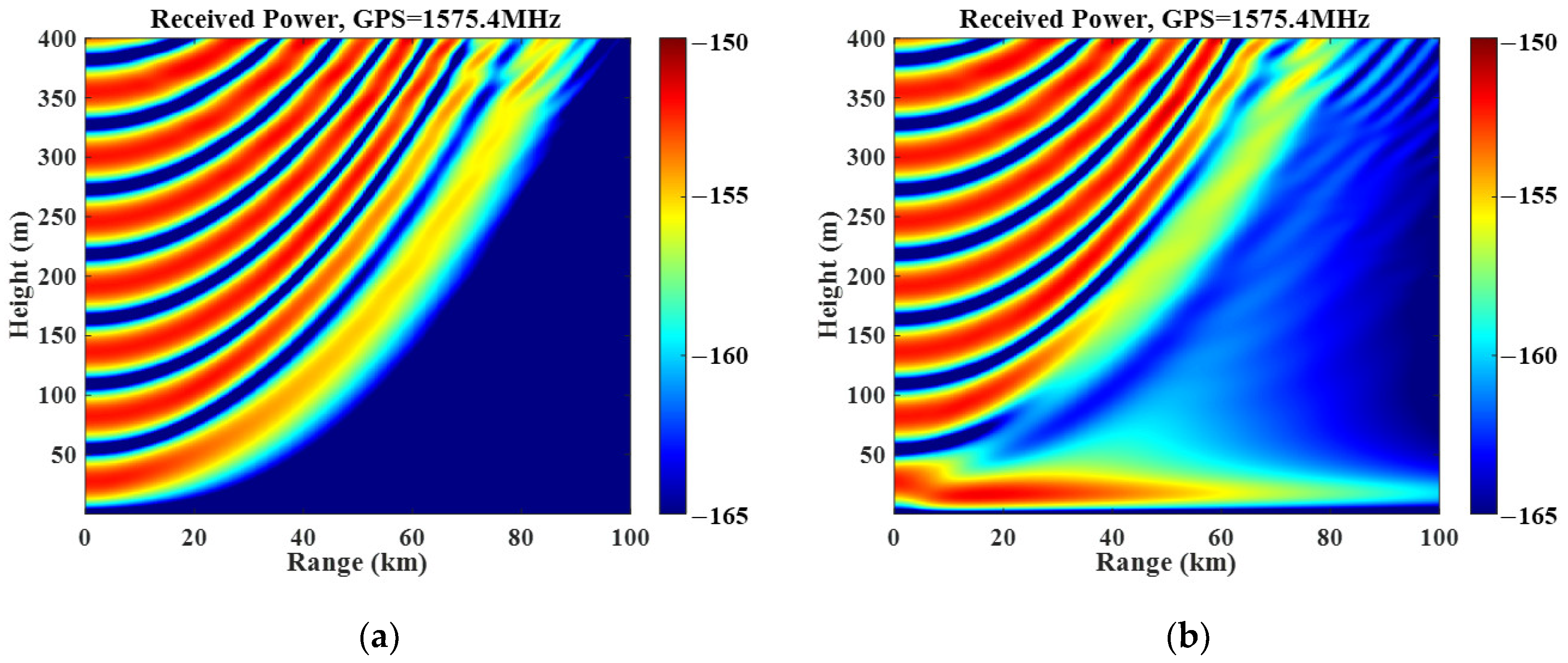
Figure 3 shows the simulation results of the received power of GPS signals in free space and when the atmospheric duct height is 30 m. The simulation results are completed in Matlab. Additionally, the parameter settings are shown in
Table 1.
The received power of the GPS receiver in
Figure 3a decreases continuously with the distance increase. In
Figure 3b, it can be seen that the electromagnetic wave trapping effect occurs at the bottom of the vertical height, and the GPS-received power decreases slowly with the increase in the distance in the trapping layer. The power distribution within the trapping layer is mainly from −150 dBW to −165 dBW. When the one-parameter evaporation duct model is used for simulation, the trapping effect of the trapping layer can be seen when the duct height is close to 50 m. The two-parameter evaporation duct model is better appropriate for the propagation modeling of GPS signals because the evaporation duct’s height is typically in the range of 40 m.
Figure 3 shows the feasibility of using the GPS signal to invert the evaporation duct. The relationship between received power and distance can be used as a dataset for the inversion of the duct parameters.
3. Deep Learning Architecture
Multiple one-layer perceptrons make up the neural network of a deep learning system that links inputs and outputs [
22]. Multiple neurons make up each layer of the perceptron. The received power data of the input GPS receiver are fitted with the duct parameters by using the nonlinear properties of neurons. The following results from the relationship between the input and output are obtained:
Among them,
and
are the output of the
ith layer and the input of the kth neuron of the layer, respectively,
and
are the weight and bias, respectively,
is the number of neurons, and
is the nonlinear activation function. A typical activation function is the ReLU function [
23]:
. The gradient vanishing problem can be effectively avoided by using ReLU. After several nonlinear transformations and activation algorithms, the neurons in the hidden layer are connected to the output layer. The neural network’s final layer, the output layer, defines a loss function to measure the discrepancy between the output and the actual value. The magnitude of the loss function represents how well the network fits the data. The more closely the output value approaches the actual value, the smaller the loss function value. Updates to network weights and biases are made using the loss function value as an indicator. For the problem of GPS inversion of the evaporation duct, the mean square error function (MSE) is used as the loss function [
24]:
where
is the predicted value of the duct parameters of the network,
is the input value of the duct parameters, and
N is the number of refractive index profiles that make up the training dataset.
The Adam optimization method is used to update network parameters. By establishing the initial parameters, the method determines the loss function value. It feeds the value back to the network so that it may adjust to various weights and enhance the gradient update. The neural network achieves a better loss function value over repeated iterations [
25].
There are some deviations between the measured data and the forward calculation data in the actual atmospheric environment due to noise. Therefore, a dropout layer is added to the hidden layer to improve the model’s generalization ability. In dropout, neurons are randomly dropped from the network with a certain probability. This randomness ensures that the network is not over-influenced by some neurons, making the model somewhat resistant to noise [
26]. After adding dropout, Equation (8) becomes:
where
is a vector of 0 and 1 randomly generated from the Bernoulli distribution. During training,
is randomly generated to 0 with a given probability, so that the neuron fails in the link between input and output.
4. Inversion of Evaporation Duct Parameters Based on Deep Learning
4.1. Dataset
It is necessary to create the GPS-received power dataset that corresponds to the duct parameters when inverting the refractive index profile of the evaporation duct using deep learning. The predicted values are obtained after network fitting, and the refractive index profile will be plotted. We calculate the received power at different distances at a receiving height of 20 m using the forward propagation model of
Section 2 as input. The GPS satellite system parameters necessary for the forward model are listed in
Table 1.
We constructed the dataset using typical values for the evaporative ducts’ parameters. The duct height
value for the two-parameter evaporation duct model runs from 5 to 40 m, while the slope
value ranges from 0 to 0.5 M/m. Latin Hypercube Sampling (LHS) takes 350 samples over the duct height range and 100 samples over the slope range to produce 35,000 atmospheric refractive index profiles. This sampling technique divides the parameter space into N evenly spaced subsets, randomly chooses the duct parameters in an interval, takes values once in each interval, and then repeats this process N times to obtain a uniformly distributed duct parameter set [
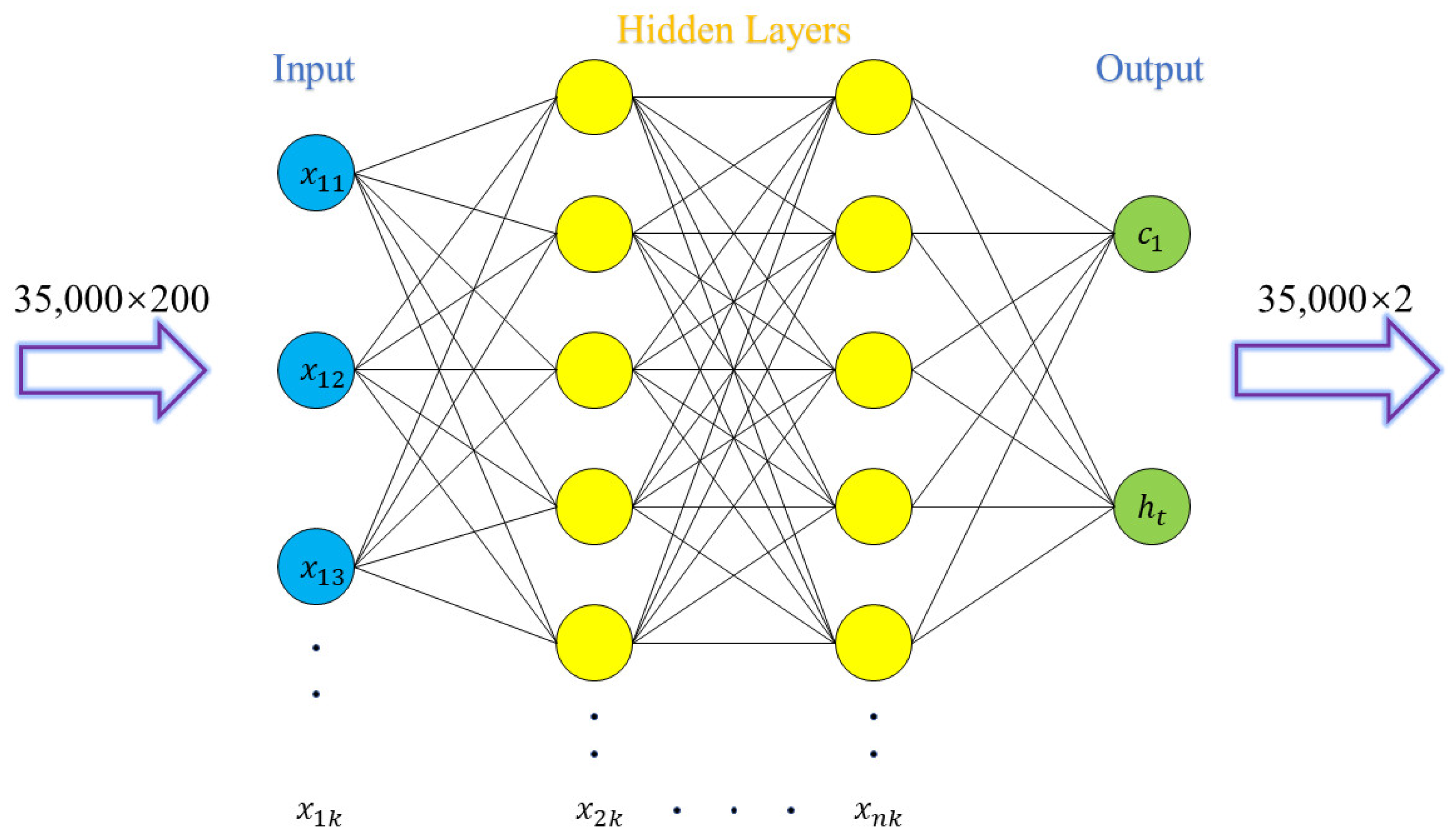
27]. We take values every 200 m over a horizontal distance of 10 to 50 km while substituting 35,000 atmospheric refractive index profiles into the forward model for simulation. The training set of 35,000 × 200 corresponds to the target set of 35,000 × 2. The deep learning network structure is depicted in
Figure 4.
Evaluation of the neural network’s performance is displayed on the validation set. There are 8750 different refractive index profiles due to the duct height taking values from 5 to 40 m at intervals of 0.1 m and the slope taking values from 0.15 to 0.4 m at intervals of 0.01 m. The validation set for performance evaluation was created by repeating the training set development process.
Inputs smaller than 0 for the ReLU activation function have a value of 0, and the neuron does not update the network weight. By using the analysis in
Section 2, it is determined that the data distribution is concentrated between −150 and −165. A dataset generated in this way may cause a neural network with a ReLU activation function to lose its ability to fit nonlinear relationships of parameters. We normalize the training and validation data to range from 0 to 1 on the same scale, shuffling the order of the datasets.
4.2. Training
In this study, the weights are initialized randomly to give the neural network various starting weights. After the neural network has undergone forward feedback training, the nonlinear relationship between the input and the output is fitted to produce weights tailored to the neurons in each layer. One of the preventative measures against overtraining is the establishment of early stopping conditions. When the weight has been modified within the maximum number of iterations, record the minimum value of the validation set loss function. The network weight update is stopped during the training phase when the validation loss value has not changed for more than 200 iterations, and the weight corresponding to the optimal loss value is returned and saved.
The Adam optimization method can adjust the learning rate during the training process. The learning rate indicates the magnitude of each weight update in the direction of the minimum value of the loss function in the nonlinear fitting. The higher the initial learning rate, the wider the weight value update step, and the easier it is to miss excellent values. Conversely, the lower the learning rate and the shorter the update step, the easier it is to overfit. We optimize its initial configuration by using the learning rate as a hyperparameter. Adam has an excellent ability to balance the size of the learning rate during training dynamically. The Adam technique, which uses Mini-batch, avoids using up a large amount of memory to accommodate complete sample input. A memory explosion would result from 35,000 sets of samples being sent into the network at once for a dataset that was created using GPS signal propagation power in an evaporation duct. The mini-batch input method enhances the benefits of deep learning on the GPU running in parallel, reduces the length of time required to train a neural network, as well as the variability of the training loss value, and makes it more stable. The neural network training is finished with Keras.
4.3. Hyperparameter Optimization
Varied neural network hyperparameter settings have different effects on network performance. The initial learning rate, number of hidden layers, number of hidden layer neurons, dropout, and other hyperparameters are suitable for the dataset size; a better output will be achieved. In order to finalize the hyperparameter settings, we employ Bayesian optimization. Hyperparameter optimization identifies the hyperparameters that, within selected limits, minimize the objective function. Bayesian optimization is based on the prior probability distribution and parameter acquisition function through the iterative search for the best value. The best value distribution of the objective function based on the prior probability is then used as the posterior probability to update the subsequent generation of parameter acquisition. With a priori probability, the following iteration is used once more, and the objective function value will advance in the desired direction [
28]. A Gaussian process is applied to create a prior probability distribution and improve flexibility. The advantages of Bayesian optimization over manual search, random search, and grid search methods include superior prior probabilities and fewer sampling times, which speed up the discovery of hyperparameters with the best values of the objective function.
As the goal of Bayesian optimization, the validation set’s loss function is searched. In this study, the hyperparameters of the Initial Learning Rate, Number of Hidden Layers, Number of Neurons, and Dropout are tuned and searched. The number of Bayesian optimization iterations is set to 10, and for each generation of training three times, the training outcome is determined by taking the validation loss’s minimal value. Three model structures are displayed in
Table 2, along with the optimization results.
The three models in
Table 2 all originated from the same time of Bayesian optimization, and there are some similar processes and outcomes. Therefore, a representative model 1 was chosen for analysis.
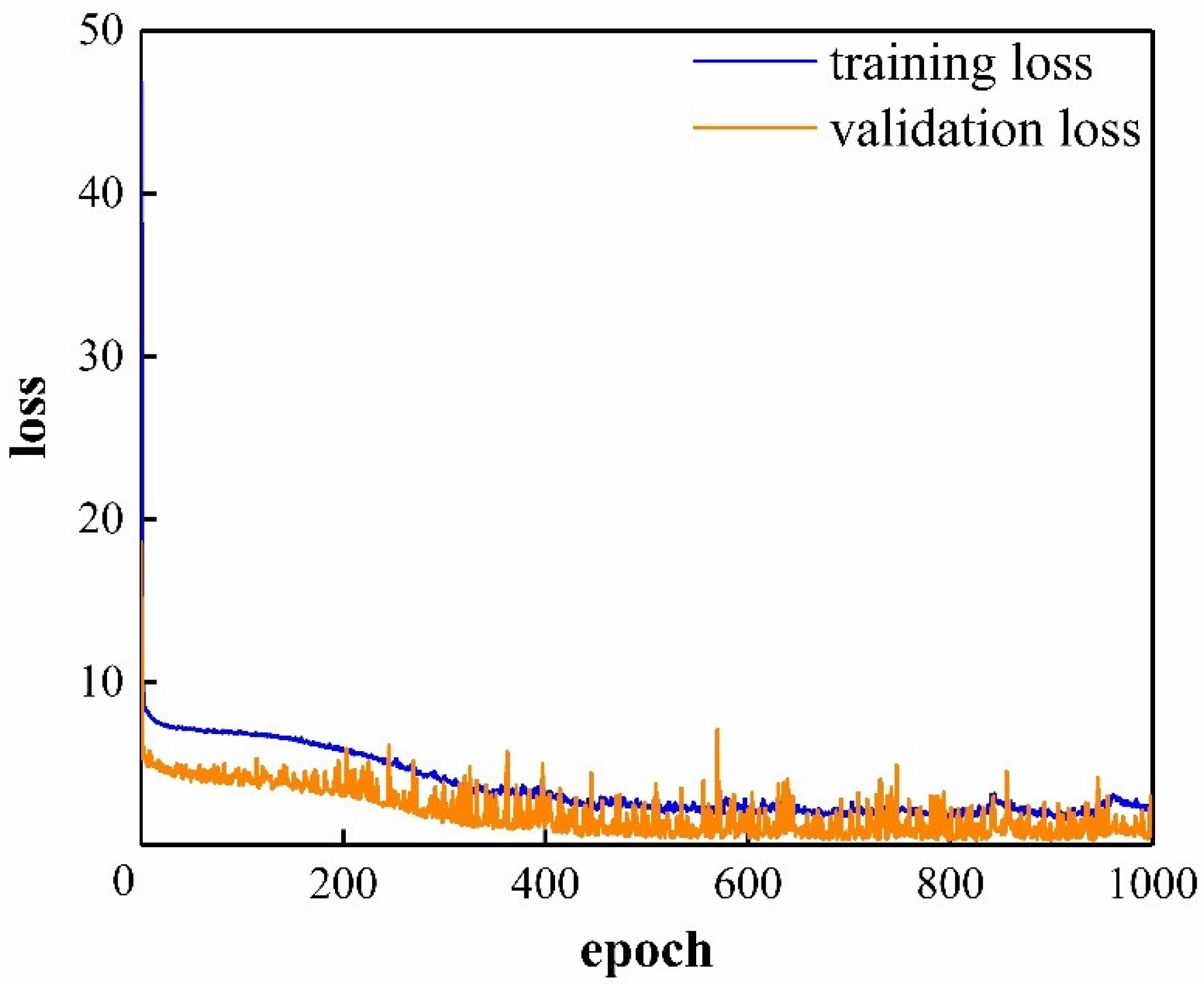
Figure 5 illustrates the sharp decline in loss value. Although the curve varies slightly due to the small batch sample input approach, it is relatively steady overall. It can be seen from a comparison of the verification loss curve and the training loss curve that the verification loss is typically lower than the training loss, which is also shown in
Table 2. This finding suggests that the network training is perfect and has a good capacity for generalization.
For the 35,000 × 200 dataset in this study, four or more hidden layers are often set when manually setting hyperparameters according to prior knowledge [
29]. However, the setting of the number of hidden layers is wholly handed over to Bayesian optimization to obtain better network performance. We set the number of hidden layers to 6. After each hidden layer, dropout is still added and selected by Bayesian optimization along with other hyperparameters. It ensures that other hyperparameters are not considered when focusing on the number of hidden layers.
Table 3 shows the optimal model structure of Bayesian optimization when six hidden layers are set, and the loss function curve is shown in
Figure 6.
Figure 6 illustrates the overfitting problem. As the number of iterations climbs, the training loss continuously declines, but the validation loss rises after the drop. When comparing
Figure 5 and
Figure 6, it is clear that whether or not the number of hidden layers is Bayesian optimized significantly impacts the training outcomes. This phenomenon results from blindly adjusting the number of hidden layers based on false experiences.
We compare the RMSE of the Bayesian optimization model with two hidden layers and six hidden layers. When the number of hidden layers is two, the model performs better and produces better outcomes. When the loss function curves are compared, it can be seen that the two-layer hidden layer has a more significant fitting effect and a more stable curve. In contrast, the six-layer hidden layer’s curve exhibits significant fluctuations, and the model becomes increasingly apparent as overfitting. An increase in hidden layers corresponds to a rise in the number of neurons participating in the neural network fitting. This leads to an overfitting stage after an initial fast fitting. Each feature value in the dataset excessively influences the loss value during the overfitting stage, making it simple to fall into the optimum local value. So, the validation set on unknown data displays significant fluctuations. The network hierarchy is excessively deep and prone to overfitting when the training loss curve falls and the validation loss curve rises, which is the case when these two curves diverge. The dropout setting currently has a negligible impact on the network.
4.4. Predict
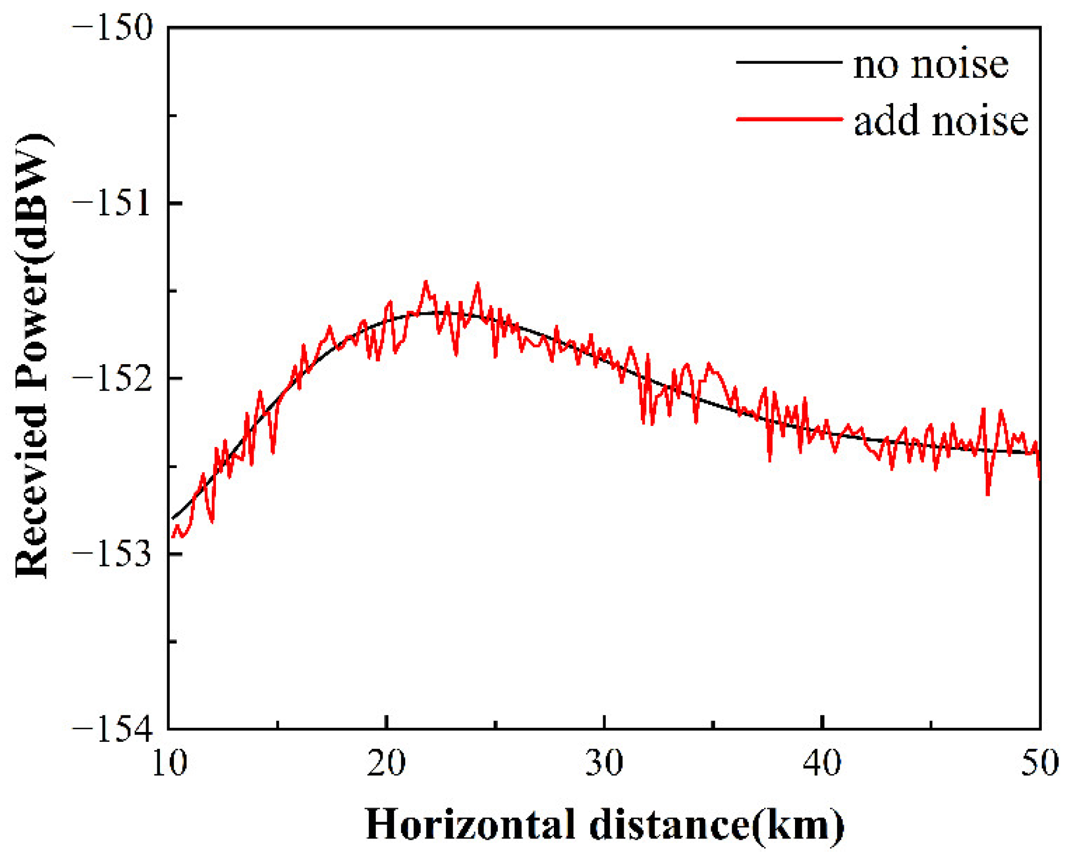
We predicted parameters using a refractive index profile at 35.7 m duct height and 0.29 M/m slope.
Figure 7 shows the received power of the GPS signal at a horizontal distance of 10 to 50 km under the duct model and the received power after adding Gaussian white noise.
The received power curve given in
Figure 7 is used as the prediction data to invert the duct parameters. The noise immunity and stability of the network structure are verified by adding noise interference. Model 1 for prediction is compared with the particle swarm optimization algorithm (PSO). The prediction results are shown in
Table 4.
Table 4 demonstrates that even though the mean relative error of Model 1 rises when noise is added to the predicted data, it remains below 1%. It is demonstrated that the neural network structure suggested in this study has good anti-noise performance while inverting the duct, that all errors are within an acceptable range, and that the predicted time increases rapidly with added noise. However, compared to PSO, it has higher accuracy and faster prediction speed.
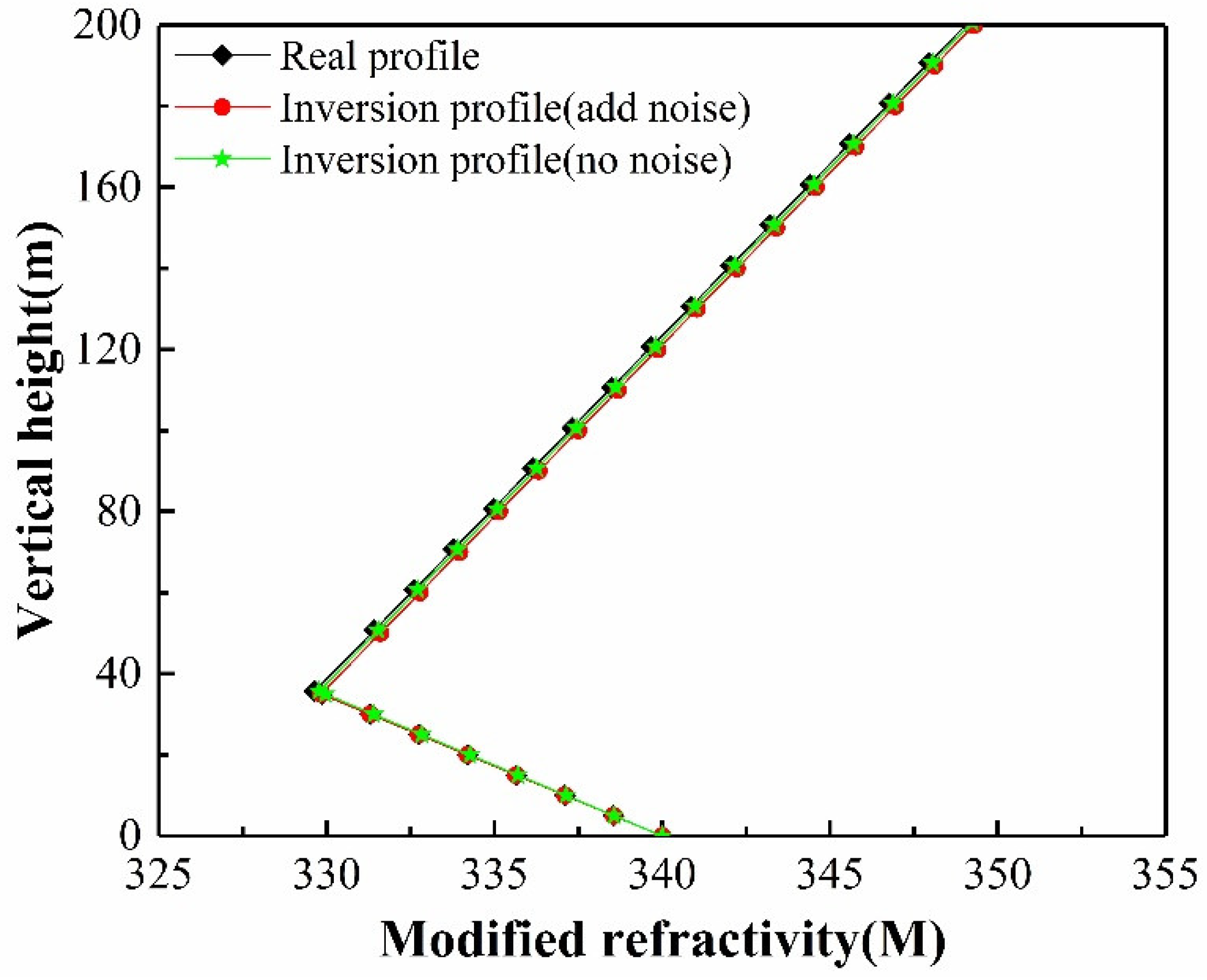
We enter the inversion-derived duct parameters under noise interference into Equation (2) and draw, as shown in
Figure 8.
Figure 8 shows that even in the presence of noise interference, the Bayesian optimized deep learning model’s evaporation duct prediction results are near the simulation results. As a result, the deep learning method for GPS signal inversion has the qualities of high precision, quick speed, good noise immunity, and strong stability.


