Article

A Novel Komodo Mlipir Algorithm and Its Application in PM2.5 Detection

School of Computer Science, Yangtze University, Jingzhou 434023, China
*
Author to whom correspondence should be addressed.
Atmosphere 2022, 13(12), 2051; https://doi.org/10.3390/atmos13122051
Submission received: 12 November 2022 / Revised: 28 November 2022 / Accepted: 5 December 2022 / Published: 7 December 2022
(This article belongs to the Special Issue Machine Learning in Air Pollution)

Abstract

:
The paper presents an improved Komodo Mlipir Algorithm (KMA) with variable inertia weight and chaos mapping (VWCKMA). In contrast to the original Komodo Mlipir Algorithm (KMA), the chaotic sequence initialization population generated by Tent mapping and Tent Chaos disturbance used in VWCKMA can effectively prevent the algorithm from falling into a local optimal solution and enhance population diversity. Individuals of different social classes can be controlled by the variable inertia weight, and the convergence speed and accuracy can be increased. For the purpose of evaluating the performance of the VWCKMA, function optimization and actual predictive optimization experiments are conducted. As a result of the simulation results, the convergence accuracy and convergence speed of the VWCKMA have been considerably enhanced for single-peak, multi-peak, and fixed-dimensional complex functions in different dimensions and even thousands of dimensions. To address the nonlinearity of PM2.5 prediction in practical problems, the weights and thresholds of the BP neural network were iteratively optimized using VWCKMA, and the BP neural network was then used to predict PM2.5 using the optimal parameters. Experimental results indicate that the accuracy of the VWCKMA-optimized BP neural network model is 85.085%, which is 19.85% higher than that of the BP neural network, indicating that the VWCKMA has a certain practical application.

1. Introduction

The metaheuristic algorithm is a type of optimization method that is based on biological cluster behavior or natural phenomenon rules. Since metaheuristic algorithms possess the characteristics of flexibility, simplicity, and efficiency, they have been widely used to solve problems such as the traveling salesman problem [1,2], the robot path planning problem [3,4], the workshop scheduling problem [5,6], and a wide range of other complex optimization problems with remarkable effects. The concept of intelligent optimization algorithms has been widely known since the mid to late 20th century. The Particle Swarm Optimization [7,8] (PSO) algorithm, for example, simulates the foraging behavior of birds, the Ant Colony Optimization [9] (ACO) algorithm simulates the foraging behavior of ants, while natural selection in evolutionary theory is the source of inspiration for the Genetic Algorithm [10,11] (GA). The rapid development of information technology has led to the development of more and more intelligent optimization algorithms to meet actual needs. Relevant scholars have proposed the following algorithms, including the Sparrow Search Algorithm [12] (SSA) based on sparrow foraging behavior and anti-predation behavior, the Grey Wolf Optimizer [13] (GWO) algorithm, which simulates the rank and predation mechanism of the grey wolf, the Whale Optimization Algorithm [14] (WOA) based on the predation behavior of the humpback whale, the Dwarf Mongoose Optimization [15] (DMO) algorithm, which mimics the foraging behavior of the dwarf mongoose, the Slime Mould Algorithm [16] (SMA) based on the oscillation mode of slime mould, the Barnacle Mating Optimizer [17] (BMO) algorithm, which mimics the mating behavior of barnacles, the Galactic Swarm Optimization [18] (GSO) algorithm, which is inspired by the motion of stars within galaxies, the Search And Rescue [19] (SAR) algorithm, which imitates the exploration behavior of humans during a search, and the Komodo Mlipir Algorithm [20] (KMA), which simulates Komodo dragon foraging and mating behavior, etc. Furthermore, metaheuristic algorithms that combine deep learning and neural networks for hyperparameter tuning have always been a hot topic in research. For example, CKH (Chaotic Krill Herd) algorithms are proposed to select the optimal parameters of the following algorithms, such as support vector regression [21] (SVR), BP neural network based on improved particle swarm optimization [22], and twin support vector machine based on improved artificial fish swarm algorithms [23]. It is also possible to optimize the parameters of deep learning models, such as convolutional neural network optimized based on artificial fish swarm optimization [24] and stacking network, which is optimized by particle swarm optimization algorithm [25].
The Komodo Mlipir Algorithm (KMA) is a novel metaheuristic optimization algorithm that was proposed by Suyanto et al. [20] in January 2022. The design is based on the behavior of Komodo monitor lizards located on Komodo Island and the Lesser Sunda Islands near Flores and the Mlipir motion. The KMA is based on swarm intelligence inspired by the social hierarchy, foraging, and reproduction of the Komodo dragon in nature. In small males, KMA used Mlipir motion as a higher exploration strategy, combining the characteristics of the Genetic Algorithm and Particle Swarm Optimization algorithm. Depending on the quality of the large males, females can choose to reproduce sexually (exploitation) or asexually (exploration). Males of large size can choose to attract one another (exploitation) or repel one another (exploration). As a final point, self-adaptation is proposed as a means of controlling the balance between exploitation and exploration and increasing the diversity of species. KMA can balance exploration and exploitation effectively, can have faster convergence speed, and can accurately converge to the optimal value by using adaptive population. However, KMA still has the problem of local convergence in the solution of complex functions, such as converging to a local optimum in the Rastrigin function. In the in-depth discussion of the Komodo Mlipir Algorithm, it is discovered that the importance of large males, small males, and females in the KMA is the same, but in the normal social hierarchy, the three classes should have different levels of importance. Consequently, the algorithm occasionally falls into the local optimal solution, and the convergence result deviates from the global optimal.
An improved Komodo Mlipir Algorithm with variable inertia weight and chaos map (VWCKMA) is proposed in this paper to further enhance the performance of KMA. In terms of higher-dimensional reference functions, VWCKMA has been demonstrated to be stable. There are three main contributions of the study. (1) By introducing time-varying inertia weights, the social class of each Komodo dragon is given an inertia weight, which increases the convergence rate of the population and enhances global exploration ability. (2) A Tent chaotic mapping approach is employed to initialize the Komodo dragon population in order to enhance the quality of the initialized population position. (3) The Tent chaotic model is employed in order to generate a few local solutions and compare them with the current solution. The algorithm will dynamically escape the local optimum if the local solution is better than the current one. As a result, the population will be more diverse, and the VWCKMA will be able to adjust the diversity of the population.
Section 3 introduces the standard KMA, and Section 4 presents the Tent mapping initialization population, the variable weight governing equation, and the Tent chaos perturbation. Section 5 discusses the experimental setup and comparison of functional optimization experiments. Section 6 presents the practical application of optimized BP neural networks for the prediction of PM2.5. Section 6 summarizes the findings and suggests future research directions.

2. Basic Komodo Mlipir Algorithm

The Komodo dragon is a leftover species from the age of dinosaurs, belonging to the family of Varanidae, living on the Komodo Islands and the Lesser Sunda Islands near Flores. Komodo dragons are ferocious, and males occasionally prey on weaker siblings and larvae and can even forage for food several kilometers away. Male monitor lizards fight to decide who will mate. Komodo dragon females are occasionally parthenogenetic; that is, they do not need males to produce offspring.
In the Komodo Mlipir Algorithm, the social hierarchy, foraging, and reproduction of the Komodo dragon are simulated. n Komodo dragon individuals were classified as large males, females, and small males based on their fitness (qualities). In the KMA, large and small males are optimized by their movements, and females are optimized by their reproduction. A concept of Mlipir is introduced in the Komodo Mlipir Algorithm. In small groups of males, in addition to foraging for themselves, they will commonly hunt for leftovers from large male Komodo dragon individuals to feed on. However, this behavior carries the risk of predation by large males, so they evade this hazard to feed safely. We call this behavior Mlipir, the movement of small males.
First, low-quality large males are attracted by high-quality large males, while high-quality large males are attracted or rejected by low-quality large males with a 0.5 probability of gaining a new position. According to the mathematical model, large males behave as follows:
V i j = r 1 ( k j k i )   if   f ( k j ) < f ( k i )   or   r 2 < 0.5 r 1 ( k i k j )   otherwise
k i = k i + j q V i j , where   j i ,
where f ( k j ) and f ( k i ) are represent the fitness (or quality) of the j and i large males, respectively. k j and k i represent the positions ( j i ) of the j and i large males, r 1 and r 2 represent the random numbers in the interval [0, 1] in the normal distribution, respectively, and q represents the number of large males.
Second, the exploitation by mating a female with a large male of the highest quality to produce two offspring, or the exploration by doing parthenogenesis. Mathematically, the mating process (sexual reproduction) of two individuals can be described as follows:
k i l = r l k i l + ( 1 r l ) k j l k j l = r l k j l + ( 1 r l ) k i l
where k i l and k j l represent the highest quality large male and female in the l dimension, k i l and k j l represent the two offspring of the l dimension produced by the mating process of the highest quality large male and female, and r l represents the random numbers in the interval of the l dimension normal distribution [0, 1].
In order to achieve parthenogenesis procedure (asexual reproduction), a small value is assigned to each female Komodo dragon’s individual dimension. A small value is generated randomly using a symmetric normal distribution and is mathematically defined as follows:
( k i 1 , k i 2 , , k i m ) ( k i 1 , k i 2 , , k i m )
k i j = k i j + ( 2 r 1 ) α | u b j l b j |
where k i 1 , k i 2 , , k i m l b j , u b j represents the position vector of k Komodo dragon individual in the m dimension, l b j and u b j represent the lower bound and upper bound of the j dimension, respectively, r represents a random value in normal distribution and α represents a parthenogenesis radius, and is set to a fixed value of 0.1. As a result, new solutions can be generated within 10% of the search space radius.
Third, in mathematical terms, the movement of small males by randomly selecting a portion of them to approach the large male can be described as follows:
V i j = l = 1 m r 1 ( k j l k i l ) i f   r 2 < d 0 otherwise
k i = k i + q j = 1 V i j ,   where   j i ,
where r 1 and r 2 represent the random numbers in the interval [0, 1] in the normal distribution, k i l and k j l represent the i small male and j large male in the l dimension, d represents the mlipir probability, l represents the dimension randomly selected based on the normal distribution, q represents the number of large males.
To summarize, the optimization process of the KMA can be described as follows: randomly generate Komodo dragon populations and determine three different classes of large males, females, and small males. The final optimization process is accomplished by moving the three classes in different directions.

3. Improvements of Basic Komodo Mlipir Algorithm

3.1. Proposed Initialization of Position by Chaotic Sequence

Chaotic mapping is a random and irregular motion. Random initialization of particles is used in most algorithms, but this may lead to an uneven distribution of particles. A chaotic sequence is characterized by ergodicity and inherent randomness in space; it can repeat irregular ergodicities within a certain range, jump out of local optimal solutions, and achieve global optimization. In recent studies, it has been demonstrated that the optimization efficiency of a swarm intelligence algorithm optimization can be greater than that of a random algorithm when chaos theory is applied, and the Tent Chaos Model has a higher ergodic property compared to the Logistic Chaos Model [26]. As a result, this paper utilizes the Tent chaotic mapping model.
Tent mapping has a simple structure, and its iterative process makes it suitable for running on a computer. There is a greater degree of ergodic uniformity in it. In this paper, the population is initialized using a Tent chaotic mapping model. Equation (8) expresses the Tent chaotic mapping model mathematically as follows:
α i j t + 1 = 2 α i j t α i j t ( 0 , 0.5 ]   2 ( 1 α i j t ) α i j t ( 0.5 , 1 ]
where t represents the number of iterations, i = 1 , 2 , , n . n represents the population size, j = 1 , 2 , , d , and d represents the dimension size. α i j t represents a chaotic variable on the j dimensional component of the i particle.
The Tent mapping method is used to generate a randomly distributed initial population to guarantee the randomness of individuals in the initial population. As a result, the search area for individual Komodo dragons is broadened and the diversity of group locations is reinforced.

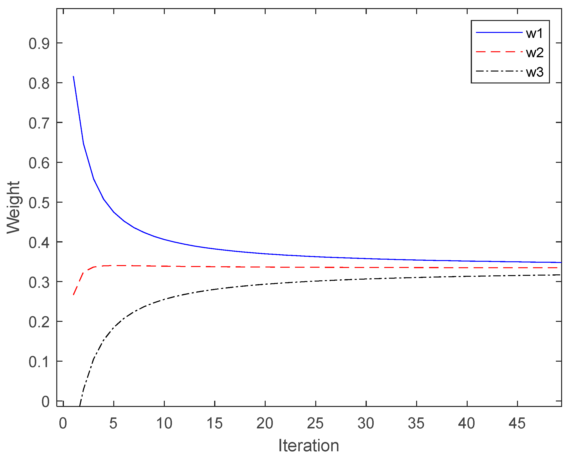
3.2. Proposed Variable Weight Strategy

The importance of large males, small males, and females in the KMA is the same, but in the normal social hierarchy, the three classes should have different levels of importance. Thus, the KMA occasionally falls into the local optimal solution. For the purpose of preventing the KMA from falling into the local optimal value during search, a new parameter called inertia weight is introduced into the original Komodo Mlipir Algorithm. In this paper, this new parameter controls the speed and individual optimum, thus affecting both global exploration and local search. When it comes to the motion of large males, females, and small males, different inertial weights, w 1 , w 2 and w 3 are introduced, respectively. The first step is to vary all the weights and add them up to 1.0.
w 1 + w 2 + w 3 = 1
For large males, females, and small males, the inertia weight should always be w 1 w 2 w 3 . During the initial iteration of determining the global optimal value, the global exploration has a greater influence. As the number of iterations increases, the influence of local optimization increases at the later stage of the process, so the inertia weight should change as well. During the iteration process, the weight of large males should be reduced from 1.0 to 1/3. Meanwhile, female reproduction and the movement of small males following large males are examples of local search. The weight of and will be increased from 0.0 to 1/3. A control inertia weight equation is presented in this paper. The cosine function is used to describe w 1 , and the angle θ is limited between 0 , arccos 1 / 3 . For w 2 , when the number of iterations is 0, w 2 and w 3 approach 0. When the number of iterations approaches , w 1 , w 2 and w 3 weight approaches 1/3. Thus, the parameter is introduced, which is expressed mathematically as follows:
φ = 1 2 arctan ( i t e r )
Due to the fact that the limiting angle θ falls between 0 , arccos 1 / 3 and w 2 will approach from 0 to 1/3 as the number of iterations increases. It is assumed that w 2 contains sin θ and con φ , and θ should be from 0 arccos ( 1 / 3 ) . The mathematical expression is as follows:
θ = 2 π arccos 1 3 arctan ( i t e r )
There is a new variable weight location update method proposed, which is defined as follows:
w 1 = cos θ , w 2 = 1 2 sin θ cos φ , w 3 = 1 w 1 w 2 ,
The varying weight curve is illustrated in Figure 1.
As a result, there has been an improvement in the mathematical expression (1) of large male movement as follows:
V i j = w 1 V i j + r 1 ( k j k i )   if   f ( k j ) < f ( k i )   or   r 2 < 0.5 w 1 V i j + r 1 ( k i k j )   otherwise
where k i and k j represent different large males, r 1 and r 2 represent a random number between [0, 1], and w 1 represents the inertia weight of large males.
According to the original KMA, females can only reproduce sexually or asexually. The new movement of the female toward the large male is in accordance with the normal physiological activity in nature. In essence, this movement is intended to move toward the direction of large males for local exploration in order to determine the optimal value. This movement can be expressed mathematically as follows:
V i = w 2 V i + r k j k i , where   j i , k i = k i + V i
where k i and k j represent females and the largest males, respectively; r represents a random number between [0, 1], and w 2 represents the inertia weight of females. k i represents the new female position.
In a similar manner, the movement of small males is improved by adding inertia weight, i.e., Equation (6) is improved. Therefore, the mathematical expression for the position movement of small males is as follows:
V i j = w 3 V i j + l = 1 m r 1 ( k j l k i l ) i f   r 2 < d 0 otherwise
where r 1 and r 2 represent the random numbers in the interval [0, 1] in the normal distribution; k i l and k j l represent the i small male and the j large male in the l dimension, respectively; d represents the specific probability; l represents the dimensions randomly selected based on the normal distribution, and w 3 represents the inertia weight of small males.

3.3. Proposed Tent Chaos Disturbance Strategy

After the movement of the three classes of Komodo is completed, that is, in the case of global exploration, chaotic disturbance is executed to achieve local search. This paper uses the Tent chaotic model for perturbation to generate some local solutions around the Komodo volume, which are then compared with preceding solutions. The specific Tent chaotic local search steps are as follows:
Step 1: Set k = 0, randomly generate a random number m of [0, Dim], which means that chaotic search is conducted on dimension m, and randomly generate a random variable α i j t of [0, 1].
Step 2: Via Equation (8) to generate chaotic variable α i j t + 1 , generate a local solution around the ith individual in the jth dimension: x i j t + 1 = α i j t + 1 × x i j t j = 1 , 2 , , m .
Step 3: Determine whether x i j t + 1 meets the constraint conditions and standardize them within the specified range.
Step 4: Calculated fitness of x i j t + 1 . In the event that the local solution is superior to the original solution, the obtained local solution will replace the original particle, and if a solution superior to the original particle cannot be generated after reaching the maximum chaotic time, the local solution will be discarded; otherwise, k = k + 1, return to step 2.

3.4. VWCKMA Process

Step 1: Initialize the parameters. The size of the population and dimension, the maximum and minimum iterations, radius of parthenogenesis, the probability value of the mlipir, and the maximum amount of chaos.
Step 2: Initialize the population. Komodo dragon individual groups are initially positioned using Tent mapping.
Step 3: Calculate the fitness values of Komodo dragon individuals and the inertia weights of Komodo dragon of different social classes by using Equations (9)–(12).
Step 4: Update the position of large males according to Equations (2) and (13). Then, update the position of females based on Equations (3)–(5) and (14), as well as the position of small males based on Equations (7) and (15).
Step 5: Use Equation (8) to conduct a local search and generate a local solution: x i l = α i j t × x i j , where i = 1 , 2 , , n , n represents the population size, j = 1 , 2 , , d , and d represents the dimension size. Determine whether x i l meets the constraint conditions, and limit the solution to the variable range.
Step 6: Calculated fitness value of x i l . If the obtained local solution is superior to the original solution, the obtained local solution replaces the original particle, and if a solution superior to the original particle cannot be generated after reaching the maximum chaotic times, the local solution is discarded. Otherwise, return to Step 5.
Step 7: Execute Step 8 after determining that the optimal solution is obtained or that the maximum number of iterations is reached; otherwise, return to Step 3.
Step 8: Output the optimal value information.
VWCKMA flow is illustrated in Figure 2.

4. Time Complexity Analysis

The time complexity of the standard Komodo Mlipir Algorithm is represented by O ( n × m × M a x _ i t e r a t i o n ) , where n , m and M a x _ i t e r a t i o n represent the number of individuals in the population, the dimension, and the maximum number of iterations. The following is an analysis of the time complexity of VWCKMA:
(1) The time complexity of Tent mapping initialization population is represented by O ( n × m ) , then the time complexity of the algorithm introducing Tent mapping initialization population is represented by O ( n × m × M a x _ i t e r a t i o n + n × m ) = O ( n × m × M a x _ i t e r a t i o n ) .
(2) Assuming that the time required to update the time-varying inertia weight is represented by t 1 , the time complexity of the algorithm after introducing the time-varying inertia weight is represented by O ( n × m × M a x _ i t e r a t i o n + t 1 ) = O ( n × m × M a x _ i t e r a t i o n ) .
(3) The disturbance time complexity of the Tent chaotic model is represented by O ( n × m ) , so the time complexity of the disturbance algorithm using the Tent chaotic model is represented by O ( n × m × M a x _ i t e r a t i o n + n × m ) = O ( n × m × M a x _ i t e r a t i o n ) .
To summarize, As compared with the standard KMA, the proposed VWCKMA has a similar time complexity, which does not increase the algorithm’s complexity.

5. Empirical Studies

The purpose of the experiments is to verify the advantages of VWCKMA by comparing it with the standard KMA and other metaheuristic algorithms. Optimization algorithms are used to optimize benchmark functions that are modeled by humans describing real problems they actually encounter.

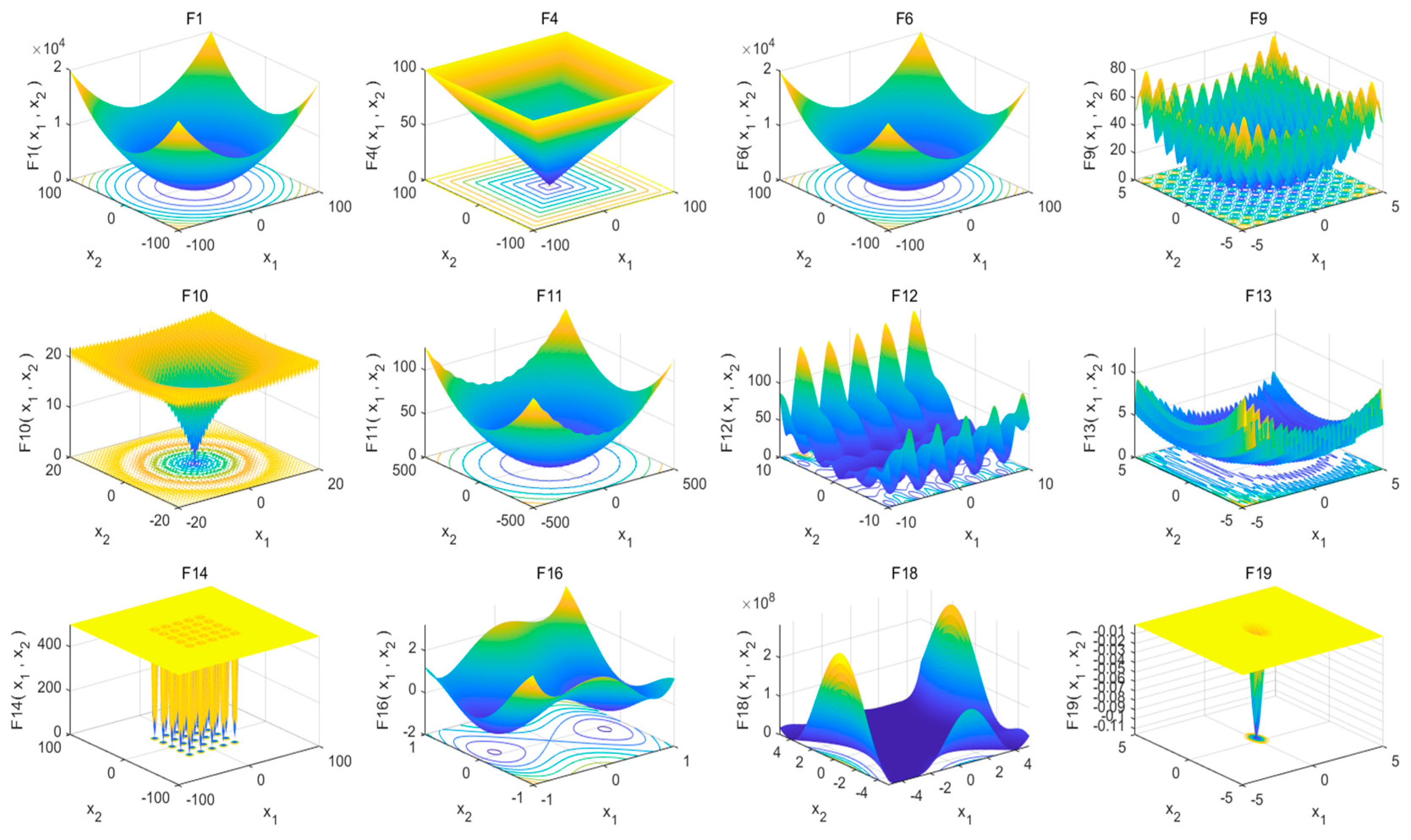
5.1. Benchmark Functions

A benchmark function is a function that is produced by natural research. It is difficult to solve them using analytical expressions because they are usually diverse and unbiased. Historically, benchmark functions have been an important method for verifying the efficiency, effectiveness, and reliability of algorithms. Test functions are important to verify and compare the performance of optimization algorithms [27].
The benchmark function is a set of functions to test the performance of the evolutionary computing algorithm. The benchmark functions are described in detail by Yao Xin et al. [28]. For the purpose of testing the effectiveness, superiority, and the convergence accuracy of complex benchmark functions in high dimensions of VWCKMA, we choose 20 benchmark functions from the literature [29], including seven unimodal functions ( f 1 ( x ) ~ f 7 ( x ) ), six multimodal functions ( f 8 ( x ) ~ f 13 ( x ) ), and seven fixed-dimensional functions ( f 14 ( x ) ~ f 20 ( x ) ). In addition to the global minimum, the F1 function also has d-dimension local minimum values, which are continuous, concave, and unimodal. The F9 function, called the Rastrigin function, has numerous local minima. In two-dimensional form, the F10 function is characterized by an extremely flat outer area and a large hole in the center. The introduction of the F10 function puts the optimization algorithm at risk of getting stuck in numerous local minima. The F11 function, called the Griewank function, has numerous local minima that are regularly distributed. The rescaled form of the F18 function has a mean of zero and a variance of one and also adds a tiny Gaussian error term to the output. The three kinds of function information are shown in Table 1, Table 2 and Table 3. The typical 2D versions of the benchmark functions considered in this paper are depicted in Figure 3.

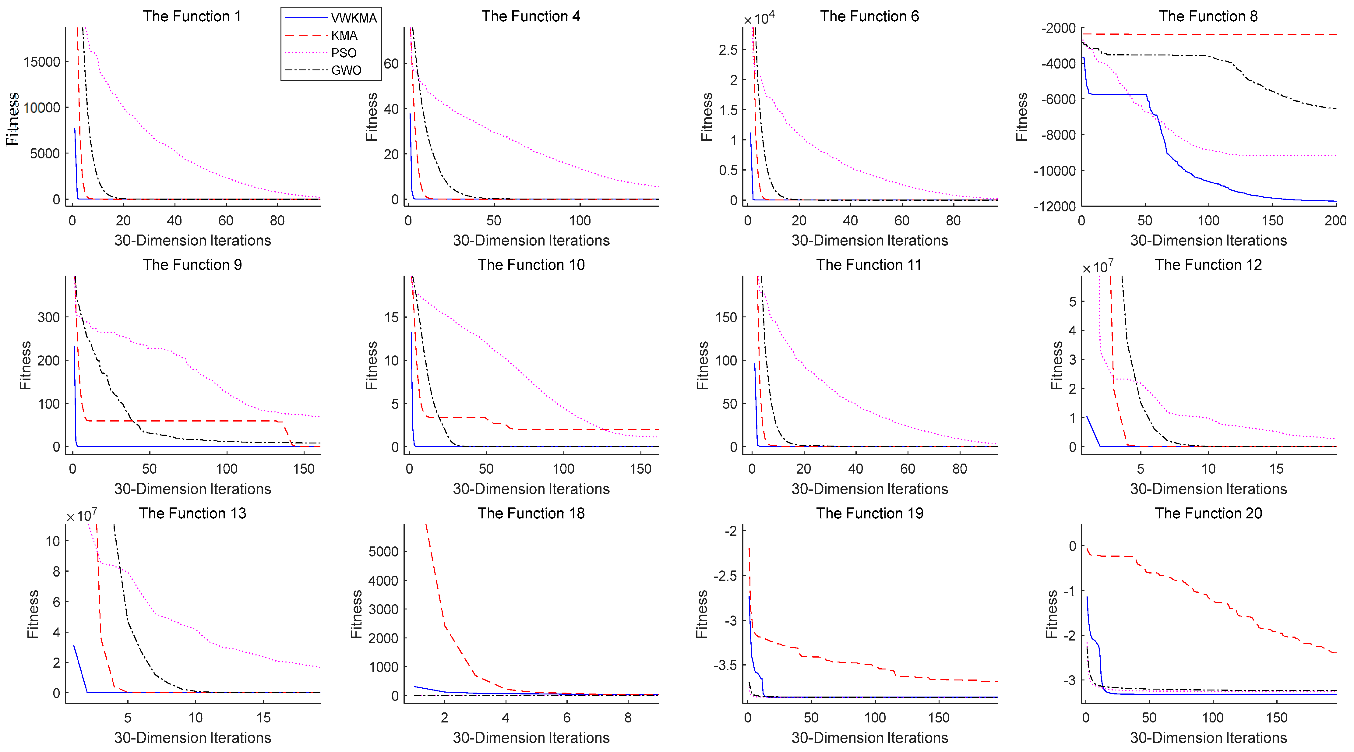
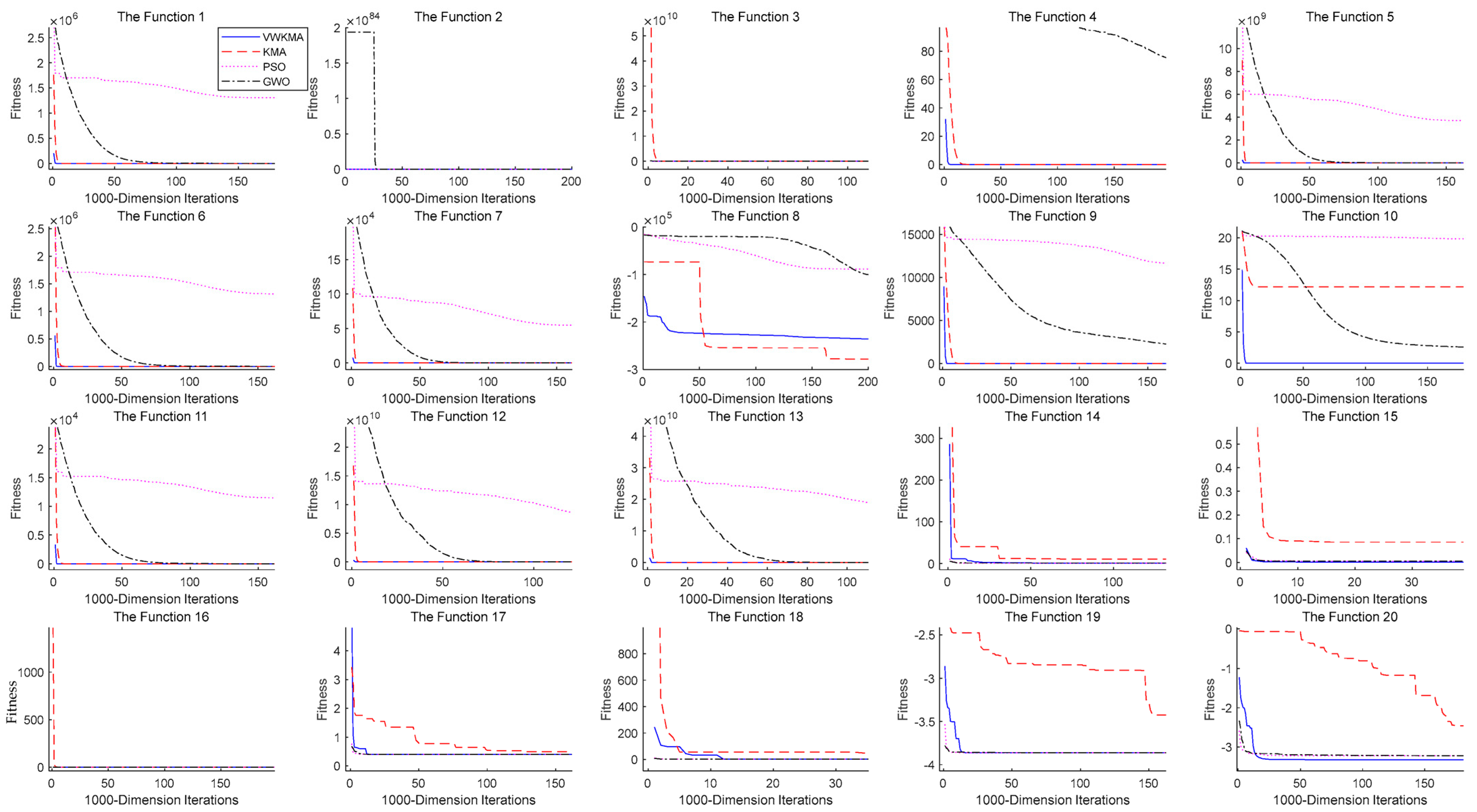
5.2. Experimental Data and Analysis

The KMA, the GWO algorithm, and the PSO algorithm are compared with the VWCKMA in this paper, and numerical simulation experiments are conducted. The involved code is written with MATLAB R2020a software, and the simulation environment is a 64-bit Windows system with an Intel Core i7-12700f 2.10GHz CPU and 32GB of RAM.
In the VWCKMA, KMA, GWO algorithms, and PSO algorithm, the maximum number of iterations is set to 200, and the maximum population size is 200. As a result, benchmark functions of 30-dimensional, 100-dimensional, 500-dimensional, and 1000-dimensional are run independently 30 times and an optimization computation is executed. The optimization solution of the fixed-dimensional functions is depicted in Table 4. As shown in Table 5, Table 6, Table 7 and Table 8, the mean and standard deviation of 7 unimodal functions and 6 multimodal functions ( f 1 ( x ) ~ f 13 ( x ) ) are calculated by different algorithms under 30 dimensions, 100 dimensions, 500 dimensions, and 1000 dimensions, respectively; the best algorithm is bold and underlined. Figure 4 depicts the convergence curves of some classic test benchmark functions in 30 dimensions to more intuitively reflect the superior performance of the VWCKMA. In order to more intuitively observe the superior performance of VWCKMA in high-dimensional situations, Figure 5 compares the convergence curves of benchmark functions of VWCKMA and other algorithms in 1000 dimensions.
The fixed-dimensional function can be a good test of the exploratory ability of the algorithm. According to the results in Table 4, VWCKMA performs well in terms of convergence accuracy, with the smallest standard deviation in the fixed-dimensional function ( f 14 ( x ) ~ f 20 ( x ) ), implying that the VWCKMA has superior convergence accuracy.
Functions f 1 ( x ) ~ f 7 ( x ) are unimodal which have only one global optimal solution and are used to evaluate the exploitation ability of the algorithm. Unlike unimodal functions, multimodal functions ( f 8 ( x ) ~ f 13 ( x ) ) contain many local optima, the number of which varies with dimension. Therefore, this multimodal test benchmark function can effectively evaluate the exploration ability of the optimization algorithm. As can be seen from Table 5, Table 6, Table 7 and Table 8, the VWCKMA has strong advantages compared with other metaheuristic algorithms. As shown in Table 5, the VWCKMA is the most efficient optimizer for f 1 ( x ) ~ f 4 ( x ) , f 6 ( x ) , and f 8 ( x ) ~ f 13 ( x ) , and is at least the second-best optimizer among the f 5 ( x ) and f 7 ( x ) test functions at the 30 dimension. Consequently, the VWCKMA has terrific exploitation ability. In Table 6, only function 7 is slightly inferior to the KMA at 100 dimensions. The optimal convergence value of the VWCKMA for f 7 ( x ) is 1 × 10⁻⁵ less than that of the KMA. The difference between the two is very small and can be ignored. It can be seen from Table 7 that the VWCKMA can converge to the theoretical optimal value of the function for f 1 ( x ) ~ f 4 ( x ) , f 9 ( x ) , and f 10 ( x ) . The convergence accuracy of the remaining functions is the highest compared to other algorithms. For the simulation experiments in 1000 dimensions shown in Table 8, in 1000 dimensions, the VWCKMA still has a high-strength convergence ability. Among the f 1 ( x ) ~ f 6 ( x ) and f 8 ( x ) ~ f 20 ( x ) , the VWCKMA is the best optimization algorithm. Compared with the f 7 ( x ) , there is little difference with the KMA. Other metaheuristic algorithms fail to converge in 1000 dimensions.
As can be seen from Figure 4, compared with other algorithms, VWCKMA has fewer convergence iterations and better convergence accuracy. The convergence speed and accuracy of the VWCKMA are better than the standard KMA. In the f 8 ( x ) ~ f 10 ( x ) and f 14 ( x ) ~ f 20 ( x ) , when KMA falls into local optimal value, VWCKMA can effectively jump out of local optimal value. The results indicate that VWCKMA has high convergence accuracy and fast convergence speed.
To conclude, VWCKMA is clearly superior to the four swarm intelligence algorithms in terms of convergence accuracy and convergence speed, as well as in terms of optimization calculation of unimodal functions and multimodal functions. In addition to its strong ability to perform global exploration and local search as well as fast convergence speeds. For high-dimensional or even thousand-dimensional conditions, it still is also highly resistant to local optimal solutions. As a result, it can jump out of the local optimal solution and find the optimal value of the function.

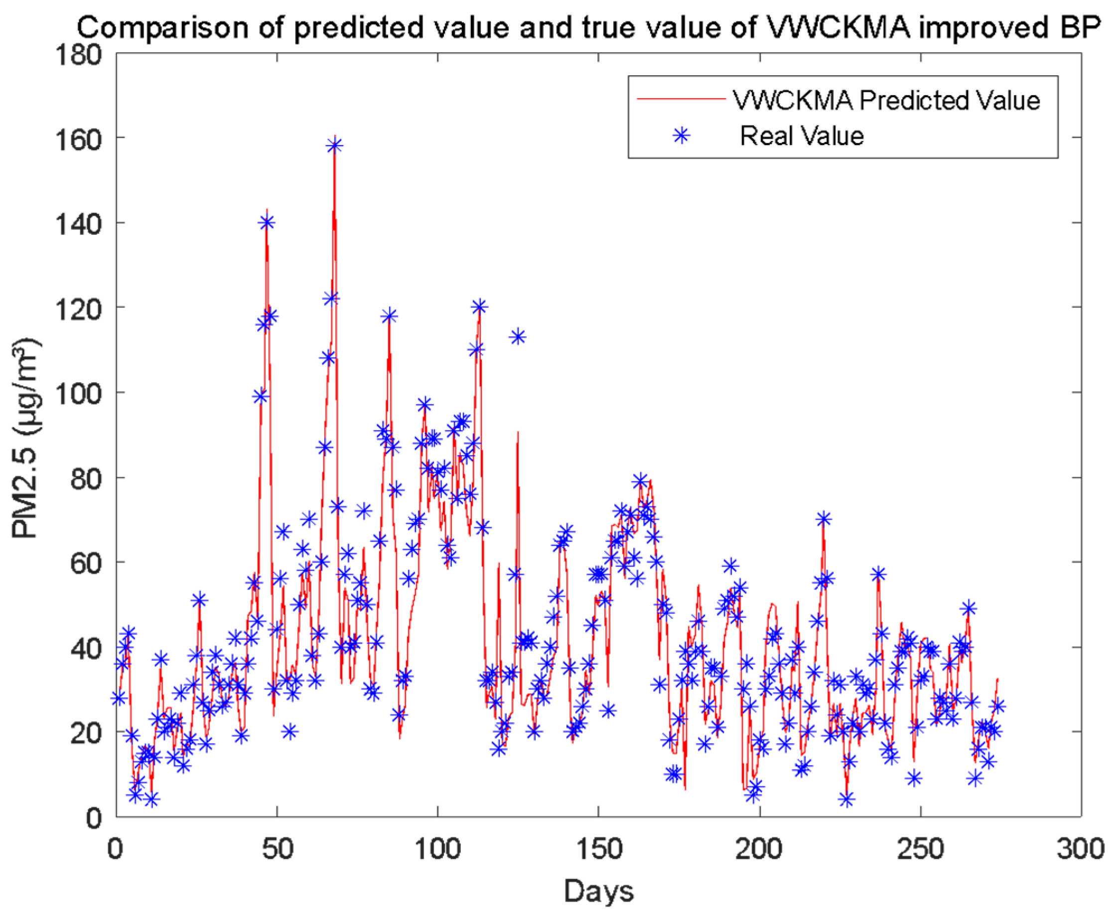
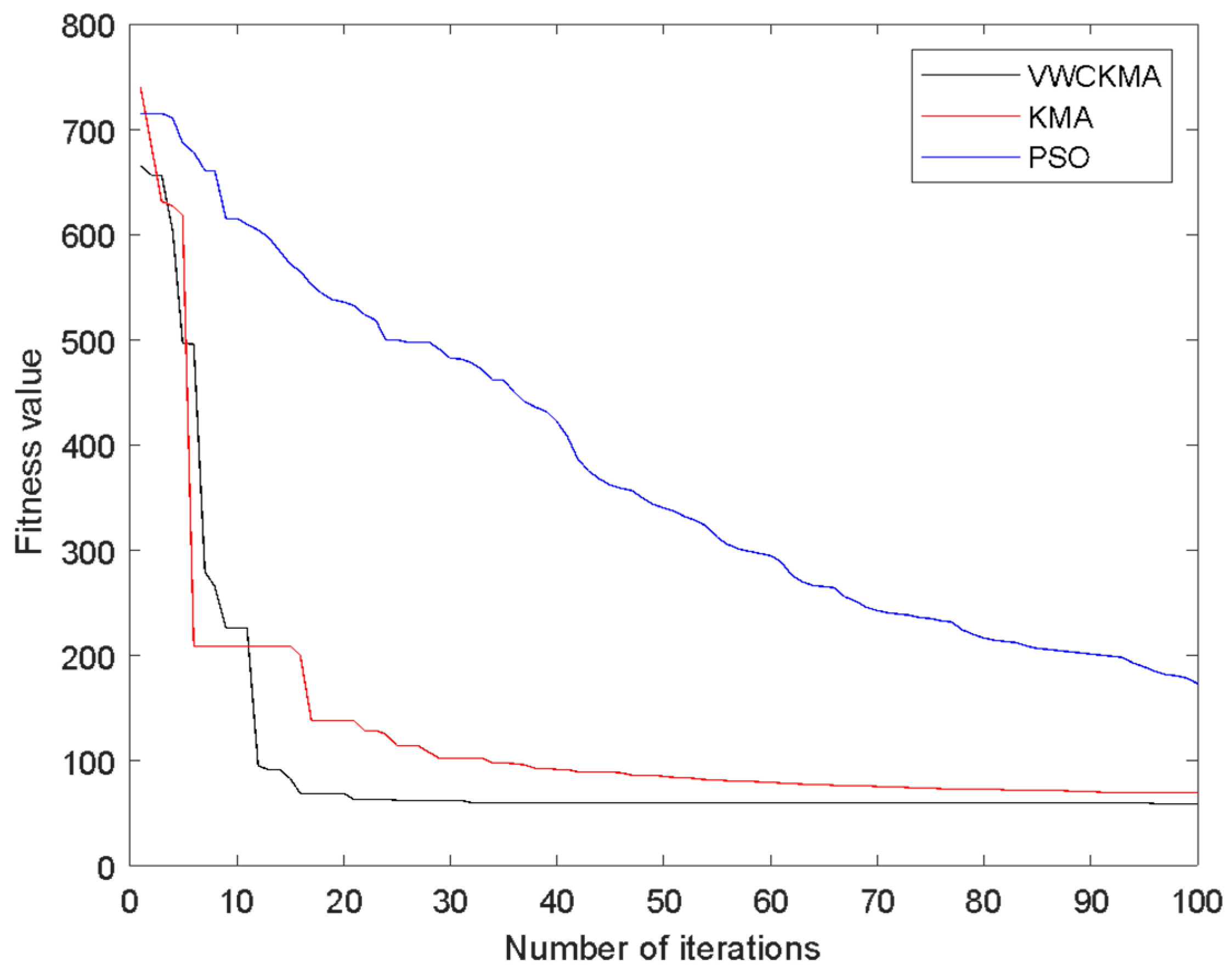
6. Practical Application

Currently, pollutant prediction models mainly consist of the following three categories: physical models [30], statistical models [31], and artificial intelligence models [32]. In this paper, the VWCKMA is applied to the prediction of PM2.5 in Chengdu. We selected five models of traditional BP neural networks [33], particle swarm optimization neural networks [34] (PSO-BP), KMA optimization BP neural networks (KMA-BP), VWCKMA optimization BP neural networks (VWCKMA-BP), and Random Forest Algorithm for Traditional Machine Learning [35] to predict air pollution PM2.5 in Chengdu using MATLAB simulation experiments. A fair comparison of the five prediction models is made. The structure of the BP neural network is 5-10-5-1, the transfer function from the input layer to the hidden layer is Tansig function, the transfer function from the hidden layer to the output layer is Poslin function, and the learning rate is 0.4. In the random forest algorithm, the number of leaf nodes is 5, and the number of trees is 200. The sample data were collected from the China air quality online monitoring and analysis platform (https://www.aqistudy.cn, accessed on 12 October 2022). In Chengdu, 912 pieces of data were selected for analysis from 1 January 2020 to 30 June 2022. There is detailed information regarding date, AQI, quality grade, PM2.5, PM10, CO, NO2, SO2, and O3. For a summary of the data, please refer to Table 9. The following data are listed due to a lack of space.
As shown in Table 9, the unit of the 6 pollutant concentration data is μ g / m 3 , and the air quality AQI is a dimensionless index. In an all-around comparison, prediction value is compared with real value. The evaluation indicators are introduced, which include the mean relative error (MAPE), the mean square error (MSE), the mean absolute error (MAE), the root mean square error (RMSE), and prediction accuracy (ACC). As the fitness function of the algorithm, the mean square error function is used in all prediction models. Each of the four indicators is defined mathematically as follows:
M A P E = 1 N j = 1 N | y i y j * | y i
M S E = 1 N j = 1 N ( y i y j * ) 2
M A E = 1 N j = 1 N | y i y j * |
R M S E = 1 N j = 1 N ( y i y j * ) 2
where N represents the number of test samples, y i represents the true value of the air quality index, and y j * represents the predicted value of the air quality index.

Results Analysis

A total of 70% of the 912 pieces of data collected from 1 January 2020 to 30 June 2022 are selected as training sets and 30% as test sets. Figure 6 illustrates the prediction comparison results of the five predictive models. The predicted value model of the VWCKMA-BP is compared to the real value, as shown in Figure 7. Table 10 presents the statistical results of MAPE, MSE, MAE, RMSE, and prediction accuracy (1-daily relative error rate = daily prediction accuracy rate, and then calculates the arithmetic mean value of all prediction samples) for the five predictive models. As shown in Table 10, different optimization strategies have a significant impact on the prediction of BP neural networks. With the VWCKMA, the accuracy rate of the improved BP neural network algorithm reaches 85.085%.
As shown in Figure 7, the BP neural network model optimized by the VWKMA is closer to the true value, and the optimization accuracy is significantly improved by the VWCKMA. Among the five models, only the VWCKMA-optimized neural network model (VWCKMA-BP) produces an average absolute error MAE that is lower than 6. The root means square error, MSE, is less than 60, the mean square error, MAPE, is less than 15%, and the accuracy rate reaches 85.085%. Figure 8 shows the comparative convergence curves for KMA, PSO, and VWCKMA. Due to the initialization population of Tent mapping, VWCKMA has better fitness values than the other two models VWCKMA is close to convergence after approximately 30 iterations, and other algorithms have a higher fitness value than VWCKMA. According to the above results, the improved KMA optimization neural network model is effective and feasible for predicting the PM2.5 index.

Author Contributions

Validation, writing original draft, M.Z.; Investigation, Writing—review and editing; L.L. All authors have read and agreed to the published version of the manuscript.

Funding

This research was funded by Ministry of Education New Generation Information Technology Innovation Project 2021, grant number 2021ITA05050.

Conflicts of Interest

The authors declare no conflict of interest.

References

  1. Lin, S.; Kernighan, B.W. An effective heuristic algorithm for the traveling-salesman problem. Oper. Res. 1973, 21, 498–516. [Google Scholar] [CrossRef] [Green Version]
  2. Grefenstette, J.; Gopal, R.; Rosmaita, B.J.; Gucht, D.V. Genetic algorithms for the traveling salesman problem. In Proceedings of the the First International Conference on Genetic Algorithms and Their Applications, Pittsburgh, PA, USA, 24–26 July 1985; pp. 160–168. [Google Scholar]
  3. Hu, Y.; Yang, S.X. A knowledge based genetic algorithm for path planning of a mobile robot. In Proceedings of the IEEE International Conference on Robotics and Automation, New Orleans, LA, USA, 26 April–1 May 2004; Volume 2004, pp. 4350–4355. [Google Scholar]
  4. Ismail, A.; Sheta, A.; Al-Weshah, M. A mobile robot path planning using genetic algorithm in static environment. J. Comput. Sci. 2008, 4, 341–344. [Google Scholar]
  5. Yin, L.; Li, X.; Gao, L.; Lu, C.; Zhang, Z. A novel mathematical model and multi-objective method for the low-carbon flexible job shop scheduling problem. Sustain. Comput. Inform. Syst. 2017, 13, 15–30. [Google Scholar] [CrossRef]
  6. Jiang, T.; Deng, G. Optimizing the low-carbon flexible job shop scheduling problem considering energy consumption. IEEE Access 2018, 6, 46346–46355. [Google Scholar] [CrossRef]
  7. Poli, R.; Kennedy, J.; Blackwell, T. Particle swarm optimization. Swarm Intell. 2007, 1, 33–57. Available online: http://d.wanfangdata.com.cn/Periodical_dqkx201507013.aspx (accessed on 10 September 2022). [CrossRef]
  8. Shi, Y.; Eberhart, R. A modified particle swarm optimizer. In Proceedings of the IEEE International Conference on Evolutionary Computation Proceedings. IEEE World Congress on Computational Intelligence (Cat. No. 98TH8360), Piscataway, NJ, USA, 4–9 May 1998; pp. 69–73. [Google Scholar]
  9. Dorigo, M.; Birattari, M.; Stutzle, T. Ant colony optimization. IEEE Comput. Intell. Mag. 2006, 1, 28–39. [Google Scholar] [CrossRef]
  10. Houck, C.R.; Joines, J.; Kay, M.G. A genetic algorithm for function optimization: A Matlab implementation. Ncsu-Ie Tr 1995, 95, 1–10. [Google Scholar]
  11. Mirjalili, S. Genetic Algorithm //Evolutionary Algorithms and Neural Networks: Theory and Applications; Springer International Publishing: Cham, Switzerland, 2019; pp. 43–55. [Google Scholar]
  12. Xue, J.; Shen, B. A novel swarm intelligence optimization approach: Sparrow search algorithm. Syst. Sci. Control Eng. 2020, 8, 22–34. [Google Scholar] [CrossRef]
  13. Mirjalili, S.; Mirjalili, S.M.; Lewis, A. Grey wolf optimizer. Adv. Eng. Softw. 2014, 69, 46–61. [Google Scholar] [CrossRef] [Green Version]
  14. Mirjalili, S.; Lewis, A. The whale optimization algorithm. Adv. Eng. Softw. 2016, 95, 51–67. [Google Scholar] [CrossRef]
  15. Agushaka, J.O.; Ezugwu, A.E.; Abualigah, L. Dwarf mongoose optimization algorithm. Comput. Methods Appl. Mech. Eng. 2022, 391, 114570. [Google Scholar] [CrossRef]
  16. Li, S.; Chen, H.; Wang, M.; Heidari, A.A.; Mirjalili, S. Slime mould algorithm: A new method for stochastic optimization. Future Gener. Comput. Syst. 2020, 111, 300–323. [Google Scholar] [CrossRef]
  17. Sulaiman, M.H.; Mustaffa, Z.; Saari, M.M.; Daniyal, H. Barnacles mating optimizer: A new bio-inspired algorithm for solving engineering optimization problems. Eng. Appl. Artif. Intell. 2020, 87, 103330. [Google Scholar] [CrossRef]
  18. Muthiah-Nakarajan, V.; Noel, M.M. Galactic swarm optimization: A new global optimization metaheuristic inspired by galactic motion. Appl. Soft Comput. 2016, 38, 771–787. [Google Scholar] [CrossRef]
  19. Waharte, S.; Trigoni, N. Supporting search and rescue operations with UAVs. In Proceedings of the International Conference on Emerging Security Technologies, Canterbury, UK, 6–7 September 2010; pp. 142–147. [Google Scholar]
  20. Suyanto, S.; Ariyanto, A.A.; Ariyanto, A.F. Komodo Mlipir Algorithm. Appl. Soft Comput. 2022, 114, 108043. [Google Scholar] [CrossRef]
  21. Zhang, Z.; Ding, S.; Sun, Y. A support vector regression model hybridized with chaotic krill herd algorithm and empirical mode decomposition for regression task. Neurocomputing 2020, 410, 185–201. [Google Scholar] [CrossRef]
  22. Sun, W.; Xu, Y. Using a back propagation neural network based on improved particle swarm optimization to study the influential factors of carbon dioxide emissions in Hebei Province, China. J. Clean. Prod. 2016, 112, 1282–1291. [Google Scholar] [CrossRef]
  23. Gao, Y.; Xie, L.; Zhang, Z.; Fan, Q. Twin support vector machine based on improved artificial fish swarm algorithm with application to flame recognition. Appl. Intell. 2020, 50, 2312–2327. [Google Scholar] [CrossRef]
  24. Goluguri, N.; Devi, K.S.; Srinivasan, P. Rice-net: An efficient artificial fish swarm optimization applied deep convolutional neural network model for identifying the Oryza sativa diseases. Neural Comput. Appl. 2021, 33, 5869–5884. [Google Scholar] [CrossRef]
  25. Wang, B.; Xue, B.; Zhang, M. Particle swarm optimisation for evolving deep neural networks for image classification by evolving and stacking transferable blocks. In Proceedings of the IEEE Congress on Evolutionary Computation (CEC), Glasgow, UK, 19–24 July 2020; pp. 1–8. [Google Scholar]
  26. Shan, L.; Qiang, H.; Li, J.; Wang, Z. Chaotic optimization algorithm based on Tent map. Control Decis. 2005, 20, 179–182. [Google Scholar]
  27. Jamil, M.; Yang, X.-S. A literature survey of benchmark functions for global optimization problems. arXiv 2013, arXiv:1308.4008 2013. [Google Scholar]
  28. Yao, X.; Liu, Y.; Lin, G. Evolutionary programming made faster. IEEE Trans. Evol. Comput. 1999, 3, 82–102. [Google Scholar]
  29. Chopra, N.; Ansari, M.M. Golden jackal optimization: A novel nature-inspired optimizer for engineering applications. Expert Syst. Appl. 2022, 198, 116924. [Google Scholar] [CrossRef]
  30. Huang, K.; Xiao, Q.; Meng, X.; Geng, G.; Wang, Y.; Lyapustin, A.; Gu, D.; Liu, Y. Predicting monthly high-resolution PM2.5 concentrations with random forest model in the North China Plain. Environ. Pollut. 2018, 242, 675–683. [Google Scholar] [CrossRef] [PubMed]
  31. Zhou, H.; Zhang, F.; Du, Z.; Liu, R. Forecasting PM2.5 using hybrid graph convolution-based model considering dynamic wind-field to offer the benefit of spatial interpretability. Environ. Pollut. 2021, 273, 116473. [Google Scholar] [CrossRef] [PubMed]
  32. An, Y.; Xia, T.; You, R.; Lai, D.; Liu, J.; Chen, C. A reinforcement learning approach for control of window behavior to reduce indoor PM2.5 concentrations in naturally ventilated buildings. Build. Environ. 2021, 200, 107978. [Google Scholar] [CrossRef]
  33. Kang, Z.; Qu, Z. Application of BP neural network optimized by genetic simulated annealing algorithm to prediction of air quality index in Lanzhou. In Proceedings of the 2017 2nd IEEE International Conference on Computational Intelligence and Applications (ICCIA), Beijing, China, 8–11 September 2017; pp. 155–160. [Google Scholar]
  34. Li, M.; Wu, W.; Chen, B.; Guan, L.; Wu, Y. Water quality evaluation using back propagation artificial neural network based on self-adaptive particle swarm optimization algorithm and chaos theory. Comput. Water Energy Environ. Eng. 2017, 6, 229. [Google Scholar] [CrossRef] [Green Version]
  35. Hu, X.; Belle, J.H.; Meng, X.; Wildani, A.; Waller, L.A.; Strickland, M.J.; Liu, Y. Estimating PM2.5 concentrations in the conterminous United States using the random forest approach. Environ. Sci. Technol. 2017, 51, 6936–6944. [Google Scholar] [CrossRef]
Figure 1. Iterative graph of time-varying weights.
Atmosphere 13 02051 g001
Figure 2. Implementation framework of VWCKMA.
Atmosphere 13 02051 g002
Figure 3. 2D representations of a typical benchmark mathematical functions.
Atmosphere 13 02051 g003
Figure 4. Comparison of the convergence curves obtained by VWCKMA and other algorithms for some benchmark functions in 30 dimensions.
Atmosphere 13 02051 g004
Figure 5. Comparison of the convergence curves obtained by different algorithms for benchmark functions in 1000 dimensions.
Atmosphere 13 02051 g005
Figure 6. Comparison of real and predicted values of different prediction models.
Atmosphere 13 02051 g006
Figure 7. Comparison of predicted and real value of the improved BP neural network by VWCKMA.
Atmosphere 13 02051 g007
Figure 8. Iterative convergence curve of the algorithm.
Atmosphere 13 02051 g008
Table 1. Unimodal test function.
FunctionRangeFmin
f 1 ( x ) = i = 1 n x i 2 [−100, 100]0
f 2 ( x ) = i = 1 d | x i | + i = 1 d | x i | [−10, 100]0
f 3 ( x ) = i = 1 n ( j 1 i x j ) 2 [−100, 100]0
f 4 ( x ) = max i [ | x i | ,   1 i n ] [−100, 100]0
f 5 ( x ) = i = 1 n 1 { 100 ( x i + 1 x i 2 ) 2 + ( x i 1 ) 2 } [−30, 30]0
f 6 ( x ) = i = 1 n ( x i + 0.5 ) 2 [−100, 100]0
f 7 ( x ) = i = 1 n i x i 4 + r a n d o m ( 0 , 1 ) [−1.28, 1.28]0
Table 2. Multimodal test function.
FunctionRangeFmin
f 8 ( x ) = i = 1 n x i sin ( | x i | ) [−500, 500] 418.9829 D i m
f 9 ( x ) = i = 1 n [ x i 2 10 cos ( 2 π x i ) + 10 ] [−5.12, 5.12]0
f 10 ( x ) = 20 exp ( 0.2 1 n i = 1 n x i 2 ) exp ( 1 n i = 1 n cos ( 2 π x i ) ) + 20 + e [−32, 32]0
f 11 ( x ) = 1 4000 i = 1 n x i 2 i = 1 n cos ( x i i ) + 1 [−600, 600]0
f 12 ( x ) = π n { 10 sin ( π y 1 ) + i = 1 n 1 ( y i 1 ) 2 [ 1 + 10 sin 2 ( π y i + 1 ) ] + ( y n 1 ) 2 } + i = 1 n u ( x i , 10 , 100 , 4 ) y i = 1 + x i + 1 4 u ( x i , k , a , m ) = k ( y i a ) m   ;   y i > a 0   ;   a > y i > a k ( y i a ) m   ; y i < a [−50, 50]0
f 13 ( x ) = 0.1 { sin 2 ( 3 π y 1 ) + i = 1 n ( y i 1 ) 2 [ 1 + sin 2 ( 3 π y i + 1 ) ] + ( y n 1 ) 2 [ 1 + sin 2 ( 2 π y n ) ] } + i = 1 n u ( y i , 5 , 100 , 4 ) [−50, 50]0
Table 3. Fixed-dimensional test functions.
FunctionRangeFmin
f 14 ( x ) = ( 1 500 + j = 1 25 1 j + i = 1 2 ( y i a i j ) 6 ) 1 [−65, 65]1
f 15 ( x ) = i = 1 11 a i x 1 ( b i 2 + b i x 2 ) b i 2 + b i x 3 + x 4 2 [−5, 5]0.00030
f 16 ( x ) = 4 x 1 2 2.1 x 1 4 + 1 3 x 1 6 + x 1 x 2 4 x 2 2 + 4 x 2 4 [−5, 5]−1.0316
f 17 ( x ) = { x 2 5.1 4 π 2 x 1 2 + 5 π x 1 6 } 2 + 10 ( 1 1 8 π ) cos x 1 + 10 [−5, 5]0.398
f 18 ( x ) = [ 1 + ( x 1 + x 2 + 1 ) 2 ( 19 14 x 1 + 3 x 1 2 14 x 2 + 6 x 1 x 2 + 3 y 2 2 ) × [ 30 + ( 2 x 1 3 x 2 ) 2 × ( 18 32 x 1 + 12 x 1 2 + 48 x 2 36 x 1 x 2 + 27 x 2 2 ) ] ] [−2, 2]3
f 19 ( x ) = i = 4 4 c i exp ( j = 1 3 a i j ( y j p i j ) 2 ) [1, 3]−3.86
f 20 ( y ) = i = 4 4 c i exp ( j = 1 6 a i j ( y j p i j ) 2 ) [0, 1]−3.32
Table 4. Comparison of different algorithms in solving the fixed-dimensional test functions.
PSOGWOKMAVWCKMA
MeanStd.MeanStd.MeanStd.MeanStd.
f 14 ( x ) 9.98 × 10−10.00 × 1001.23 × 1006.21 × 10−16.20 × 1003.59 × 1009.98 × 10−1 0.00 × 100
f 15 ( x ) 1.29 × 10−33.62 × 10−31.68 × 10−35.08 × 10−35.51 × 10−25.10 × 10−23.07 × 10⁻⁴ 3.80 × 10⁻⁹
f 16 ( x ) −1.0 × 1006.52 × 10−16−1.0 × 1001.48 × 10−8−9.4 × 10−11.27 × 10−1−1.0 × 1000.00 × 100
f 17 ( x ) 3.98 × 10−10.0 × 1003.98 × 10−14.19 × 10−44.94 × 10−13.04 × 10−13.98 × 10−10.00 × 100
f 18 ( x ) 3.00 × 1006.99 × 10−163.00 × 1003.61 × 10−61.46 × 1011.77 × 1013.00 × 1000.00 × 100
f 19 ( x ) −3.8 × 1002.71 × 10−15−3.8 × 1009.66 × 10−4−3.7 × 1003.01 × 10−1−3.8 × 1000.00 × 100
f 20 ( x ) −3.2 × 1007.57 × 10−2−3.2 × 1006.64 × 10−2−2.3 × 1007.57 × 10−1−3.3 × 1002.77 × 10−8
Table 5. Comparison of different algorithms in solving the multimodal and unimodal test functions at 30 dimensions.
PSOGWOKMAVWCKMA
MeanStd.MeanStd.MeanStd.MeanStd.
f 1 ( x ) 6.34 × 10−28.92 × 10−24.94 × 10−175.49 × 10−176.7 × 10−1352.5 × 10−1340.00 × 1000.00 × 100
f 2 ( x ) 6.51 × 1007.14 × 1001.45 × 10−107.22 × 10−113.95 × 10−721.01 × 10−710.00 × 1000.00 × 100
f 3 ( x ) 4.04 × 1034.54 × 1032.71 × 10−42.32 × 10−41.2 × 10−1076.5 × 10−1070.00 × 1000.00 × 100
f 4 ( x ) 4.22 × 1001.31 × 1001.73 × 10−48.46 × 10−51.02 × 10−653.33 × 10−650.00 × 1000.00 × 100
f 5 ( x ) 6.90 × 1021.32 × 1032.66 × 1010.86 × 1002.89 × 1011.13 × 1022.84 × 1010.14 × 100
f 6 ( x ) 1.88 × 10−16.68 × 10−11.13 × 10−11.68 × 10−15.66 × 1007.31 × 10−19.91 × 10−25.90 × 10−2
f 7 ( x ) 2.31 × 10−28.39 × 10−39.46 × 10−44.29 × 10−45.00 × 10−31.12 × 10−22.59 × 10−33.06 × 10−3
f 8 ( x ) −8.9 × 1037.94 × 102−6.6 × 1037.96 × 102−2.6 × 1038.71 × 102−1.2 × 1046.41 × 102
f 9 ( x ) 4.91 × 1011.53 × 1015.30 × 1002.531 × 1000.00 × 1000.00 × 1000.00 × 1000.00 × 100
f 10 ( x ) 1.11 × 1006.73 × 10−11.13 × 10−95.52 × 10−102.01 × 1006.12 × 1008.88 × 10−160.00 × 100
f 11 ( x ) 7.00 × 10−26.93 × 10−22.24 × 10−35.19 × 10−30.00 × 1000.00 × 1000.00 × 1000.00 × 100
f 12 ( x ) 7.76 × 10−17.03 × 10−11.07 × 10−26.49 × 10−31.22 × 1004.03 × 10−15.68 × 10−38.82 × 10−3
f 13 ( x ) 2.10 × 10−15.44 × 10−11.23 × 10−11.15 × 10−12.94 × 1001.36 × 10−14.34 × 10−23.12 × 10−2
Table 6. Comparison of different algorithms in solving the multimodal and unimodal test functions at 100 dimensions.
PSOGWOKMAVWCKMA
MeanStd.MeanStd.MeanStd.MeanStd.
f 1 ( x ) 6.86 × 1034.31 × 1033.99 × 10−61.31 × 10−66.8 × 10−1372.2 × 10−1360.00 × 1000.00 × 100
f 2 ( x ) 2.50 × 1024.62 × 1013.32 × 10−45.40 × 10−51.33 × 10−721.74 × 10−720.00 × 1000.00 × 100
f 3 ( x ) 1.02 × 1052.24 × 1058.12 × 1024.24 × 1022.2 × 10−1047.0 × 10−1040.00 × 1000.00 × 100
f 4 ( x ) 4.62 × 1013.76 × 1009.43 × 10−15.68 × 10−14.36 × 10−688.38 × 10−680.00 × 1000.00 × 100
f 5 ( x ) 8.96 × 1052.36 × 1059.82 × 1013.64 × 10−19.89 × 1017.30 × 10−29.80 × 1016.84 × 10−2
f 6 ( x ) 1.36 × 1047.92 × 1037.24 × 1008.24 × 10−11.98 × 1011.04 × 1001.84 × 1007.23 × 10−1
f 7 ( x ) 1.99 × 1011.85 × 1015.40 × 10−31.88 × 10−32.13 × 10−32.62 × 10−32.14 × 10−31.27 × 10⁻³
f 8 ( x ) −2.2 × 1041.69 × 103−1.8 × 1049.86 × 102−7.6 × 1032.38 × 103−3.6 × 1041.54 × 103
f 9 ( x ) 5.02 × 1025.04 × 1012.85 × 1011.22 × 1014.58 × 1011.45 × 1020.00 × 1000.00 × 100
f 10 ( x ) 1.10 × 1012.99 × 1002.12 × 10−45.23 × 10−51.99 × 1006.31 × 1008.88 × 10−160.00 × 100
f 11 ( x ) 8.46 × 1015.66 × 1012.90 × 10−39.15 × 10−30.00 × 1000.00 × 1000.00 × 1000.00 × 100
f 12 ( x ) 4.44 × 1039.29 × 1031.59 × 10−13.49 × 10−21.53 × 1001.57 × 1001.39 × 10−24.41 × 10⁻³
f 13 ( x ) 5.10 × 1057.95 × 1055.58 × 1007.08 × 10−19.45 × 1001.66 × 1004.63 × 10−11.38 × 10⁻¹
Table 7. Comparison of different algorithms in solving the multimodal and unimodal test functions at 500 dimensions.
PSOGWOKMAVWCKMA
MeanStd.MeanStd.MeanStd.MeanStd.
f 1 ( x ) 4.57 × 1054.58 × 1031.37 × 1019.45 × 10−13.5 × 10−1357.6 × 10−1350.00 × 1000.00 × 100
f 2 ( x ) 1.89 × 1032.99 × 1012.68 × 1001.63 × 10−18.21 × 10−701.05 × 10−690.00 × 1000.00 × 100
f 3 ( x ) 8.04 × 1041.51 × 1061.24 × 1031.38 × 1032.1 × 10−1194.6 × 10−1190.00 × 1000.00 × 100
f 4 ( x ) 6.81 × 1012.51 × 1005.83 × 1016.30 × 1051.15 × 10−652.20 × 10−650.00 × 1000.00 × 100
f 5 ( x ) 6.22 × 1053.48 × 1059.80 × 1047.24 × 10−19.89 × 1016.63 × 10−29.80 × 1014.60 × 10−2
f 6 ( x ) 2.51 × 1031.38 × 1047.60 × 1001.17 × 1001.91 × 1011.50 × 1001.28 × 1002.00 × 10−1
f 7 ( x ) 8.20 × 1031.07 × 1031.33 × 10−17.97 × 10−32.54 × 10−32.39 × 10−32.54 × 10−32.21 × 10⁻³
f 8 ( x ) −5.9 × 1042.97 × 103−6.4 × 1042.71 × 103−1.2 × 1056.03 × 103−1.3 × 1059.01 × 103
f 9 ( x ) 4.96 × 1031.03 × 10−25.35 × 1027.50 × 1010.00 × 1000.00 × 1000.00 × 1000.00 × 100
f 10 ( x ) 1.94 × 1012.54 × 10−13.70 × 10−18.72 × 10−22.01 × 1006.12 × 1008.88 × 10−160.00 × 100
f 11 ( x ) 4.18 × 1031.60 × 1029.55 × 10−11.18 × 10−10.00 × 1000.00 × 1000.00 × 1000.00 × 100
f 12 ( x ) 5.77 × 1021.30 × 1031.33 × 10−12.87 × 10−21.22 × 1001.45 × 10−11.86 × 10−27.02 × 10−3
f 13 ( x ) 5.12 × 1051.21 × 1065.54 × 1007.53 × 10−19.94 × 1001.30 × 10−14.19 × 10−15.16 × 10−2
Table 8. Comparison of different algorithms in solving the multimodal and unimodal test functions at 1000 dimensions.
PSOGWOKMAVWCKMA
MeanStd.MeanStd.MeanStd.MeanStd.
f 1 ( x ) 1.31 × 1066.15 × 1044.86 × 1026.86 × 1013.5 × 10−1336.5 × 10−1330.00 × 1000.00 × 100
f 2 ( x ) 2.23 × 1032.33 × 1013.57 × 1013.34 × 1001.27 × 10−482.20 × 10−480.00 × 1000.00 × 100
f 3 ( x ) 1.03 × 1071.14 × 1061.68 × 1063.75 × 1053.7 × 10−1028.2 × 10−1020.00 × 1000.00 × 100
f 4 ( x ) 9.91 × 1016.41 × 10−17.45 × 1012.14 × 1004.36 × 10−655.67 × 10−650.00 × 1000.00 × 100
f 5 ( x ) 3.69 × 1091.36 × 1084.13 × 1041.02 × 1049.98 × 1022.89 × 10−19.91 × 1024.25 × 10−1
f 6 ( x ) 1.32 × 1063.36 × 1047.35 × 1029.72 × 1012.17 × 1021.02 × 1013.44 × 1016.53 × 100
f 7 ( x ) 5.46 × 1045.30 × 1031.45 × 1005.25 × 10−18.23 × 10−48.94 × 10−42.68 × 10−33.37 × 10−3
f 8 ( x ) −8.9 × 1043.93 × 103−1.1 × 1054.72 × 103−2.8 × 1051.55 × 104−2.4 × 1051.21 × 104
f 9 ( x ) 1.16 × 1042.42 × 1021.63 × 1031.74 × 1020.00 × 1000.00 × 1000.00 × 1000.00 × 100
f 10 ( x ) 1.98 × 1018.90 × 10−22.52 × 1008.36 × 10−21.22 × 1011.11 × 1018.88 × 10−160.00 × 100
f 11 ( x ) 1.15 × 1044.75 × 10−25.72 × 1005.99 × 10−10.00 × 1000.00 × 1000.00 × 1000.00 × 100
f 12 ( x ) 7.29 × 1096.97 × 1087.58 × 1001.40 × 1001.01 × 1002.23 × 10−13.70 × 10−31.21 × 10−2
f 13 ( x ) 1.60 × 10101.54 × 1095.59 × 1024.10 × 101100 × 1006.53 × 10−39.07 × 1001.26 × 100
Table 9. Original data samples.
DateAQIQualityPM2.5PM10CONO2SO2O3
1 January 2020135Light103124450.9627
2 January 2020135Light1031325711022
3 January 2020105Light79102571656
4 January 2020118Light89119671.1816
29 June 2022106Light20392450.5166
30 June 202282good26503550.7138
Table 10. Statistical results of indicators.
Model M A E μ g / m 3 M S E μ g / m 3 R M S E μ g / m 3 M A P E % A C C %
BPNN12.7518280.221816.739834.762165.238
PSO-BP9.9420193.385713.906326.076373.923
KMA-BP6.427764.32318.020219.776880.223
RandomForest6.002866.71768.168116.257583.743
VWCKMA-BP5.222656.12757.491814.915285.085
Publisher’s Note: MDPI stays neutral with regard to jurisdictional claims in published maps and institutional affiliations.

