Article

Improving the Wind Power Density Forecast in the Middle- and High-Latitude Regions of China by Selecting the Relatively Optimal Planetary Boundary Layer Schemes

1
Beijing Goldwind Smart Energy Technology Co., Beijing 100176, China
2
Suntien Green Energy Co., Shijiazhuang 050051, China
3
State Grid Xinjiang Electric Power Co., Urumqi 830002, China
4
Hebei Construction & Investment Group New-Energy Co., Shijiazhuang 050051, China
5
State Grid Shandong Electric Power Co., Jinan 250001, China
*
Authors to whom correspondence should be addressed.
Atmosphere 2022, 13(12), 2034; https://doi.org/10.3390/atmos13122034
Submission received: 3 November 2022 / Revised: 21 November 2022 / Accepted: 1 December 2022 / Published: 4 December 2022
(This article belongs to the Section Meteorology)

Abstract

:
As the power generation mode with the lowest carbon emissions, wind power generation plays an indispensable role in achieving the goal of carbon neutralization. To optimize the wind power density (WPD), forecasting is crucial to improve wind power utilization and power system stability. However, because near-surface wind is characterized by notable randomness, diversity, intermittence, and uncontrollability, accurately forecasting the WPD on wind farms remains a challenging task. In this study, we attempted to improve the WPD forecast in the middle- and high-latitude regions of China (wind energy resources are abundant there) by selecting the relatively optimal planetary boundary layer (PBL) scheme, as the PBL processes exert notable effects on the near-surface wind field directly. Based on a whole month in the summer (July 2021), seven PBL schemes were compared quantitatively by using the Weather Research and Forecasting (WRF) model for a total of 70 runs (for each run, the forecast period was 3 days). The results show that no PBL schemes could always show the best performance in forecasting all variables, and the forecast accuracy showed a notable dependence on the evolution of the weather systems. Among the seven PBL schemes, the Medium-Range Forecast (MRF) scheme showed the overall best performance in forecasting the 100 m wind speed, sea level pressure, and 2 m temperature, which ensured that it had the highest forecast skill for the WPD in the middle- and high-latitude regions of China. Further analyses indicate that the background conditions were also well forecasted by the MRF scheme (ranked first or second). This was a crucial reason why the WPD forecast was the best for the MRF scheme.

1. Introduction

The kinetic energy associated with horizontal wind is referred to as wind energy [1,2]. By using specially designed blades, wind turbines absorb wind energy and convert it into electric energy [3]. This is called wind power generation. Wind energy is clean and renewable, being one of the best alternatives to traditional fossil fuel energy. According to the Fifth Assessment Report of the Intergovernmental Panel on Climate Change [4], among all the current power generation technologies, wind power generation shows the lowest carbon emissions. Therefore, to reach the goal of carbon neutralization, there is an urgent need to increase the proportion of wind power generation. Furthermore, benefits of wind energy are wide-ranging, as it contributes to sustainable job creation, public health cost savings, water consumption savings, and so on (https://gwec.net/report-capturing-green-recovery-opportunities-from-wind-power-in-emerging-economies/#) (accessed on 1 September 2022).
Although wind energy shows more advantages than traditional fossil fuel energy in many aspects, as discussed above, its limitations are also notable [3,5]. One of these is that the power generation of wind farms is difficult to predict, as wind fields are characterized by remarkable randomness, diversity, intermittence, and uncontrollability [6,7,8,9,10]. Various methods were developed to forecast the wind at the near-surface level, which can be roughly divided into two types: physical models that are mainly based on the thermodynamic and dynamic mechanisms of the atmosphere [11,12,13], and statistical models [14,15,16,17] that are mainly based on statistical features (this type includes machine learning and deep learning). For the former type, numerical models are effective and widely used tools, which can provide longer-term forecasts of wind speed and related meteorological factors than those of statistical models. Because of its advantages, a series of studies attempted to forecast wind energy by using numerical models. For instance, Bai et al. [18] evaluated the performance of the Penn State/NCAR Mesoscale Model (MM5) in forecasting the wind speed in Inner Mongolia; Zhang et al. [19] utilized the Weather Research and Forecasting (WRF) model [20] to forecast the wind energy of wind farms in Guizhou; Mughal et al. (2017) employed the WRF model to predict wind power generation in Kenya; Han and Nan [21] used the Karlsruhe Atmospheric Mesoscale Model [22] to generate high-resolution forecasts of wind energy in Europe. However, thus far, all numerical models show unignorable forecast errors, which increase the uncertainties for the accurate prediction of wind energy. Therefore, providing accurate wind forecasts at near-surface levels, particularly for the 100 m hub height (usually, the wind turbines’ hubs are at the height of 100 m), is of great importance to improve the wind power utilization and power system stability.
The planetary boundary layer (PBL) is the layer at the bottom of the atmosphere, which has the closest relationship to human activities [23,24]. All the wind turbines of wind farms are situated in this layer. Turbulence, sensible heat flux, latent heat flux, and friction dissipation in the PBL all notably affect the near-surface wind field [25]. At present, numerical models use a variety of parameterization schemes [20] to describe the main processes in the PBL. However, as different PBL parameterization schemes were developed based on different physical models and different observation data, their performances for wind forecasting in a specified area are different [13]. Therefore, to improve the wind forecast of a targeted region, it is crucial to select the relatively optimal PBL scheme for the region.
China is rich in wind energy resources [3]. To achieve the goal of carbon neutralization, the Chinese government has made efforts to speed up the development of the wind power industry [13,26], and by the end of 2021, the installed wind power capacity in China ranked first in the world. According to a 42-year statistic from Li et al. [27], for China, the areas with the most abundant wind energy on land are mainly located in middle and high latitudes, particularly for Northwest China, North China, and Northeast China. Therefore, improving the accuracy of the wind forecast in these regions is crucial for China’s wind power industry. Due to its relatively high forecasting skills, the WRF model is a widely used numerical model in wind forecasting [12,19,28,29,30,31]. It provides a series of PBL parameterization schemes [20], which affect the accuracy of wind forecasts remarkably [13]. However, to the best of our knowledge, no studies have compared the PBL parameterization schemes in forecasting wind power density (WPD) and associated factors in the middle- and high-latitude regions of China. Therefore, the primary purpose of this study is to fill this knowledge gap and to determine the relatively optimal PBL scheme for this region. This will provide a useful reference for the efficient utilization of wind energy in China.

2. Data, Model Configuration and Methods

2.1. Data

A total of four types of data were used in this study: (i) the hourly, 0.125° × 0.125° atmospheric model high-resolution 10-day forecast provided by the European Centre for Medium-Range Weather Forecasts (ECMWF; https://www.ecmwf.int/en/forecasts/datasets/set-i) (accessed on 1 September 2022) was used to generate the initial and boundary conditions for the WRF model; (ii) the hourly 0.25° × 0.25° ERA5 reanalysis data from the ECMWF (Hersbach and Dee, 2016; Huang et al., 2021), including sea level pressure, 100 m wind field, geopotential height, etc.; (iii) the observed data at the surface stations shown in Figure 1, including 10 m wind field (3-hourly), 24 h precipitation (daily), and 2 m temperature (3-hourly), were used to evaluate the performances of different PBL schemes; and (iv) the GPM IMERG Final Precipitation data (daily) [32] were used to compare the horizontal distribution of the accumulated precipitation forecasted by different PBL schemes.

2.2. Model Configuration

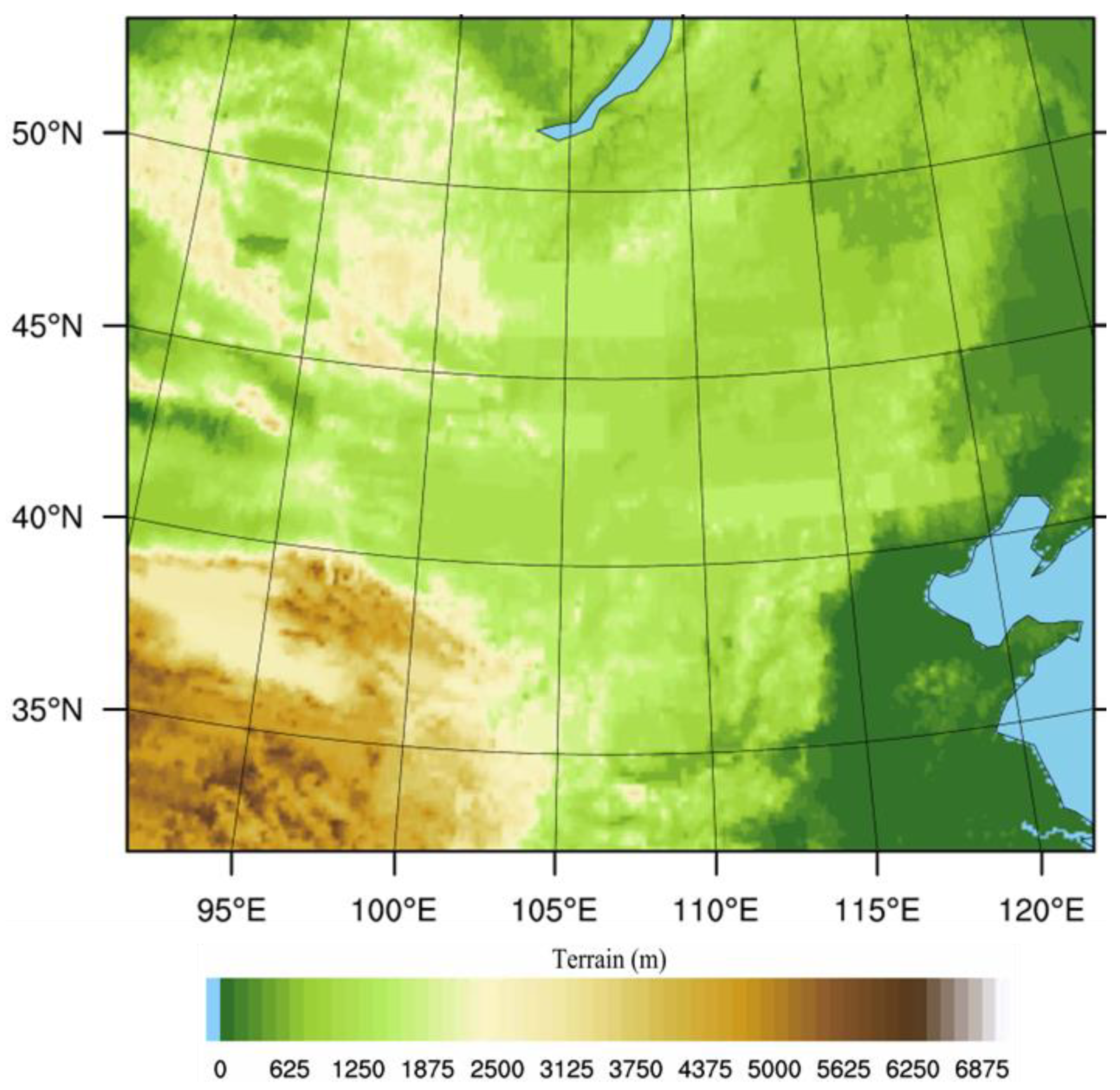
The WRF model v4.4 [20] was employed in this study. To cover the main body of the middle- and high-latitude regions of China, we used the domain shown in Figure 2 for the numerical experiments. The domain has 959 (west–east direction) × 826 (north–south direction) horizontal grids, 51 terrain-following vertical levels (top level was at 50 hPa), and a grid span of 3 km. The WRF double-moment six-class scheme [33], the Rapid Radiative Transfer Model with GCM applications scheme [34], the Dudhia shortwave scheme [35], and the five-layer thermal diffusion land surface model [36] were used in the simulations. No cumulus scheme was used in the simulations, as the grid span of 3 km is convection-permitting.
Based on previous studies evaluating the PBL schemes [13,37], a total of seven PBL schemes (Table 1) which showed adequate performances in China were compared to determine the best one for forecasting the WPD and related factors in the middle- and high-latitude regions of China. This includes the Medium-Range Forecast scheme (MRF) [33], the Mellor–Yamada Nakanishi and Niino Level 2.5 scheme (MYN) [38], the Bougeault and Lacarrere scheme (BLS) [39], the Yonsei University scheme (YSU) [40], the asymmetric convective model version 2 scheme (ACM) [41], the Grenier–Bretherthon–McCaa scheme (GBM) [42], and the University of Washington moist turbulence scheme (UWS) [43]. July of 2021 was selected as the test period for the simulations in the present study, as it ranked second in history in terms of the accumulated precipitation over the middle- and high-latitude regions of China (http://www.cma.gov.cn/2011xwzx/2011xqxxw/2011xqxyw/202112/t20211229_589812.html?from=singlemessage) (accessed on 1 September 2022). A series of rainfall events appeared during this period, which were mainly caused by the shortwave troughs and extratropical cyclones in the westerly wind, mesoscale vortices, and surface low-pressure systems [44]. Heavier precipitation tended to lower the wind forecast accuracy [45], and the results of this study can be used as a reference for this situation. Considering the huge calculation costs and the representativeness of the results, we initiated the WRF model every 72 h from 0000 UTC 1 July 2021 to 0000 UTC 31 July 2021 (i.e., at 0000 UTC on 01, 04, 07, 10, 13, 16, 19, 22, 25, and 28 July 2021), and forecasted for a 3-day period to cover the entirety of July 2021. Therefore, for each PBL scheme, there were 10 runs, and for all seven PBL schemes, there were a total of 70 runs. For convenience, 7 runs (using different PBL schemes) started at the same time were called a group—those started at 0000 UTC 1 July 2021 were named group I, those started at 0000 UTC 04 July 2021 were named group II, …, and those started at 0000 UTC 28 July 2021 were named group X (Figure 3).

2.3. Evaluation Methods

A total of seven variables (Table 2) from the forecast were evaluated to reach a comprehensive comparison of the seven PBL schemes. For the 100 m wind speed, sea level pressure, and 500 hPa geopotential height, the ERA5 reanalysis data were used for the evaluation (the WRF output data were first interpolated into a coarser resolution of 0.25° × 0.25° by using the bilinear interpolation, which was then used in evaluation). For the 10 m zonal wind, 10 m meridional wind, 2 m temperature, and 24 h precipitation, the surface observational data at the stations shown in Figure 2 were used for evaluation (the WRF output data were interpolated onto the stations shown in Figure 2).
All variables except for the 24 h precipitation were evaluated by the root mean square error (RMSE) and the correlation coefficient (COEF). The former was used to reflect the difference in values between the forecast and real situation (ERA5 reanalysis and station observation were used as the real situation); the latter was used to show how consistent the horizontal distributions of the forecast and the real situation were with each other. Their expressions are as follows:
RMSE = 1 N i = 1 N ( F i O i ) 2
COEF = i = 1 N ( F i F ¯ ) ( O i O ¯ ) / i = 1 N ( F i F ¯ ) 2 i = 1 N ( O i O ¯ ) 2
where N is the total station/grid numbers for calculation, Fi is the forecast at station/grid i, and Oi is the reanalysis/observation at station/grid i. For each 3-day run, we mainly evaluated 24-, 48-, and 72-h forecasts. After interpolating the 24/48/72 h forecasts from each 3-day run onto the ERA5 grid/station, we calculated the RMSE and COEF following Equations (1) and (2) within the targeted region. The girds/stations within the targeted region of this study must meet two requirements: the first is that they are located within the range shown in Figure 1; the second is that they belong to China. These ensure that our evaluation mainly focused on the middle- and high-latitude regions of China.
In this study, we mainly focused on the rainfall events that were no weaker than moderate rain (i.e., 24 h precipitation ≥10 mm), as their associated latent heating could notably affect the dynamic field of the atmosphere [44,45]. To evaluate the precipitation forecast, we used two factors. The first is the threat score (TS) [46], and the second is the bias score (BIAS) [47]. The former can represent how consistent the precipitation forecast is with the real situation (TS is between 0 and 1, with a larger value representing better forecast); the latter can reflect the bias of the precipitation forecast from the real situation (BIAS = 1 means the best forecast, BIAS > 1 means precipitation grids are overestimated, and BIAS < 1 means precipitation grids are underestimated). Their expressions are as follows:
TS = N A / ( N A + N B + N C )
where NA is the total number of stations where precipitation of a certain intensity appears in both the forecast and observation, NB is the total number of stations where precipitation of a certain intensity only appears in the forecast, and NC is the total number of stations where precipitation of a certain intensity only appears in the observation.
BIAS = F / O
where F is the total number of stations where precipitation of a certain intensity appears in the forecast, and O is the total number of stations where precipitation of a certain intensity appears in the observation. In order to show the precipitation bias clearly, we redefined BIAS as:
BIAS = | 1 F / O |
In this sense, BIAS = 0 means the best forecast, and a large BIAS indicates a worse forecast.

3. Evaluation on the Forecasts of Wind Power Density-Related Factors

The WPD is an effective factor to evaluate the wind energy resource available at a site. It indicates the amount of wind energy at a site that can be converted into electrical energy (measured in watts per square meter) [48]. The WPD is widely used in the field of wind power generation, and its expression [49,50] is as follows:
WPD = ρ V 3 / 2
where ρ is the air density and V is horizontal wind speed, both of which were at the 100 m hub height. From Equation (6), it can be found that to improve the forecast accuracy of WPD, we need to improve the forecasts of both ρ and V. As V3 is usually much larger than ρ, it is crucial to improve the wind speed forecast at the height of 100 m.
As documented in many studies, air density is often used as a constant. However, for the middle- and high-latitude regions of China, this is not appropriate, since many plateaus and mountains are above 1000 m or more (Figure 1). Because most numerical models do not output air density directly, we used the state equation for ideal gases to calculate it:
ρ = p / R T
where p, R, and T are the pressure, gas constant for dry air, and the temperature, respectively [25]. From Equation (7), it is clear that to improve the forecasts of ρ, we need to improve the forecast of pressure and temperature at near-surface levels.

3.1. Evaluation on the 100 m Wind Speed Forecast

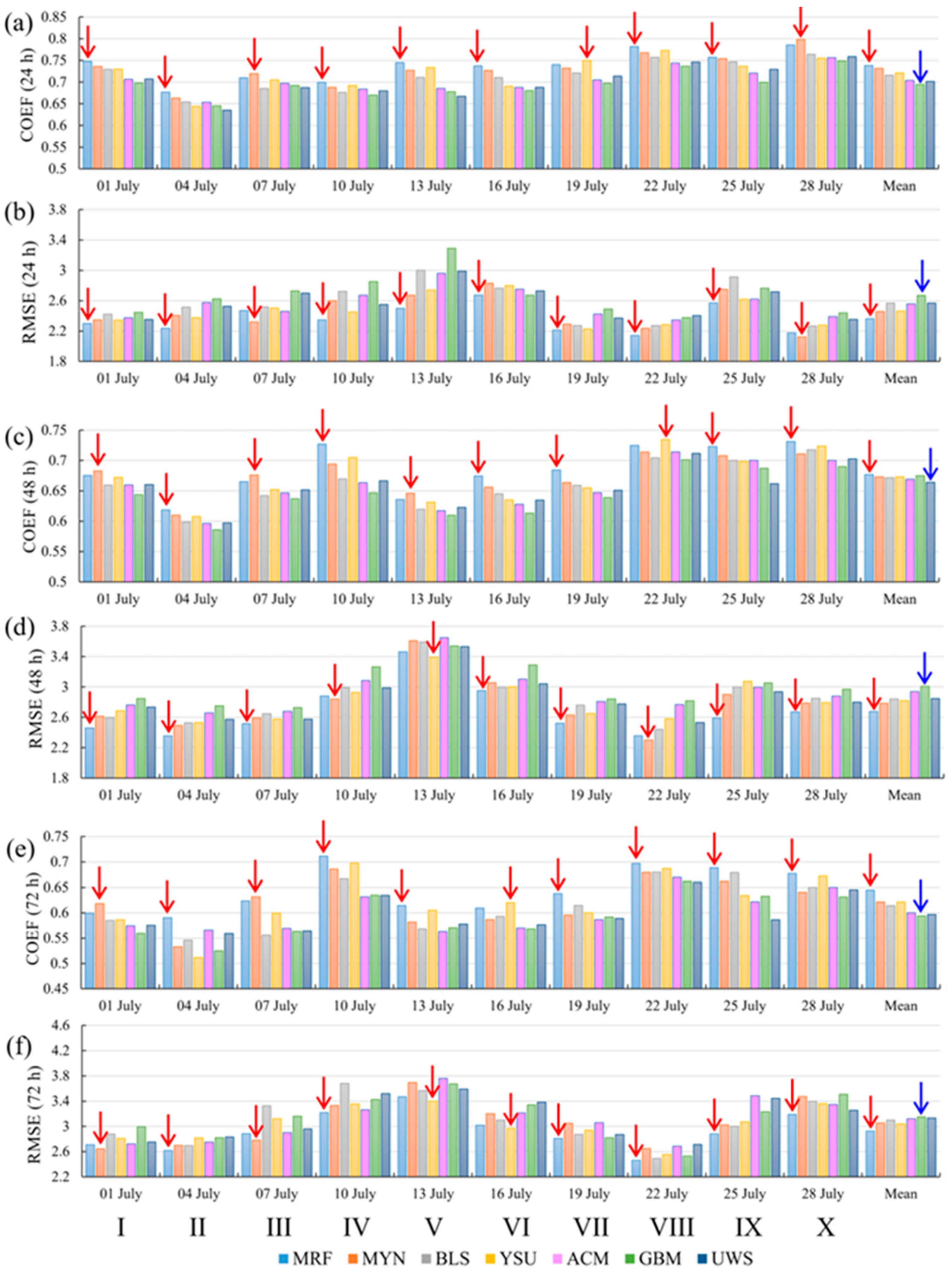
The COEFs and RMSEs of the 24-, 48-, and 72-h forecasts of the 100 m wind speed are shown in Figure 3. It is clear that for the 24/48/72 h forecast, both the COEF and RMSE were fluctuating over time, which means the forecast accuracy depended on the evolution of the weather systems. Overall, larger COEFs tended to appear with smaller RMSEs, and vice versa, implying that better/worse forecasts (larger COEF and smaller RMSE means better forecast) usually showed consistent features in COEFs and RMSEs. Moreover, comparisons among Figure 3a–f show that longer forecast times tended to have smaller COEFs and larger RMSEs, implying that the forecasts mainly became worse as the forecast time increased.
For the 24 h forecast, as Figure 3a shows, of the total 10 groups of runs, there were 7 groups where the maximum COEFs appeared in the run with the MRF scheme (I, II, IV, V, VI, VIII, and IX). For the remaining, MYN (III and X) and YSU (VII) showed the largest COEFs. In terms of RMSE, MRF had the smallest RMSEs in eight groups (I, II, IV, V, VI, VII, VIII, and IX), and the remaining minimum RMSEs appeared in MYN (III and X). Therefore, it can be concluded that for the 24 h forecast of the 100 m wind speed, the MRF scheme showed the best performance and the MYN ranked second. This can be confirmed by the mean state of the 10 groups of runs (the rightmost column of Figure 3a,b), and from the mean state, it can also be found that the YSU scheme ranked third, whereas the GBM showed the worst performance among the seven PBL schemes.
For the 48 h forecast, the MRF scheme had the largest COEFs in six groups (II, IV, VI, VII, IX, and X; Figure 3c), and the smallest RMSEs in seven groups (I, II, III, VI, VII, IX, and X; Figure 3d). Moreover, for the mean state (the rightmost column of Figure 3c,d), the MRF showed the maximum COEF and the minimum RMSE. Therefore, it is the best scheme for the 48 h forecast of the 100 m wind speed. The MYN and YSU schemes ranked second and third, respectively, in terms of the mean state.
For the 72 h forecast of the 100 m wind speed, the MRF scheme also showed the overall best performance because (i) it showed the maximum COEFs in seven groups (II, IV, V, VII, VIII, IX, and X; Figure 3e) and smallest RMSEs in six groups (II, IV, VII, VIII, IX, and X; Figure 3f), and (ii) it had the largest COEF and smallest RMSE in terms of the mean state (the rightmost column of Figure 3e,f). The MYN and YSU schemes tied for the second place in terms of mean state (Table 2).
In summary, for the forecasts of the 100 m wind speed, the MRF scheme showed the overall best performance among all seven PBL schemes (Table 2). Therefore, this scheme is strongly recommended for the 100 m wind forecast in the middle- and high-latitude regions of China.

3.2. Evaluation on the Sea Level Pressure and 2 m Temperature Forecasts

Evaluating the forecasts of sea level pressure and 2 m temperature have dual meanings: the first is that these two factors directly determine the calculation accuracy of the air density, which is indispensable to calculate the WPD, and the second is that they affect the evolution of the 100 m wind through pressure gradient force and baroclinity [1,7].
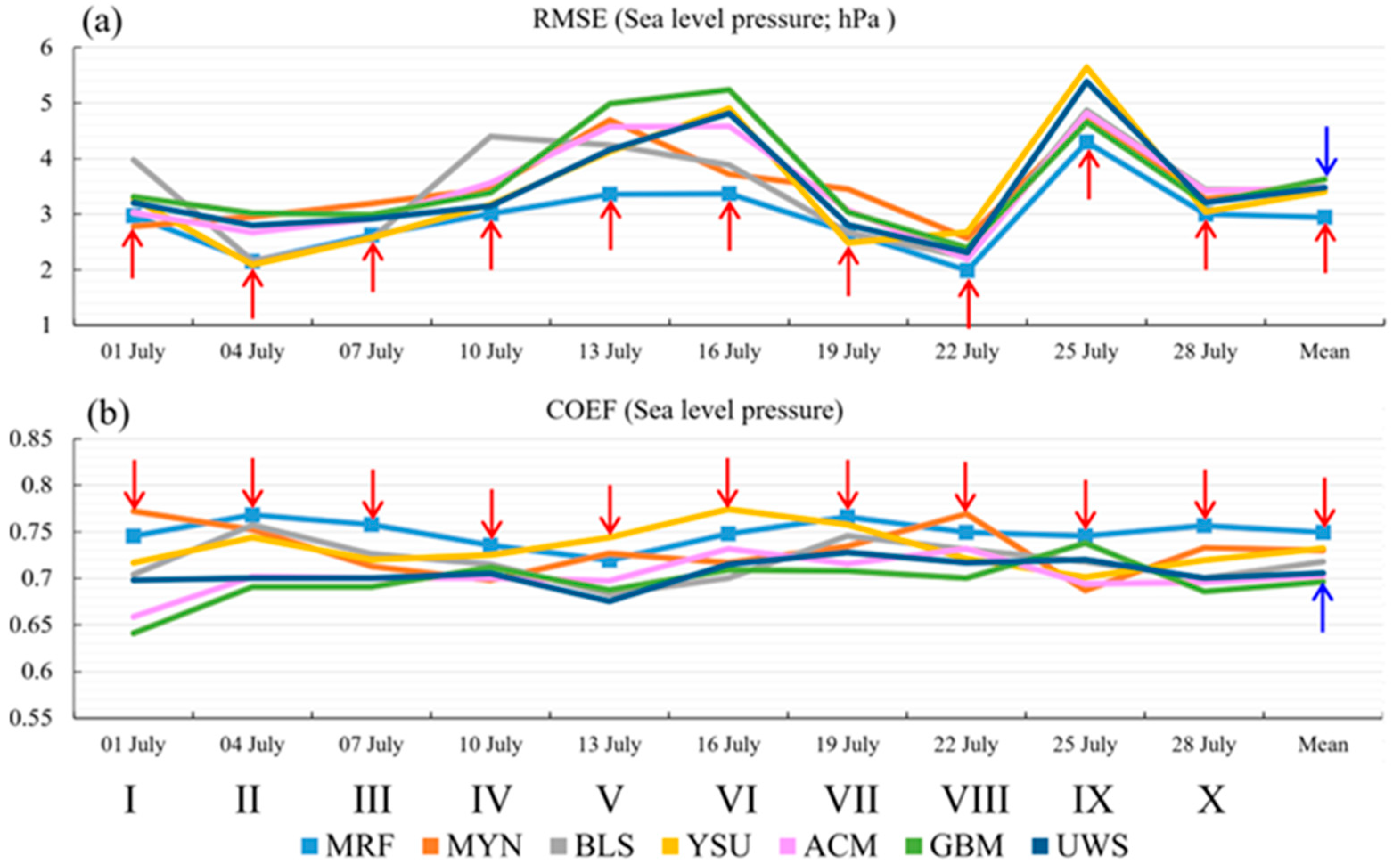
In order to obtain the overall performance of the sea level pressure forecast, we calculated the averaged RMSE (i.e., the arithmetic mean of the RMSEs for the 24 h, 48 h, and 72 h forecasts of the sea level pressure) and averaged COEF (i.e., the arithmetic mean of the COEFs for the 24 h, 48 h, and 72 h forecasts of the sea level pressure) for each PBL scheme. The results are illustrated in Figure 4. We found that the MRF scheme showed the smallest RMSEs in six groups of runs (IV, V, VI, VIII, IX, and X; Figure 4a), and it also showed the largest COEFs in six groups of runs (II, III, IV, VII, IX, and X; Figure 4b). Moreover, in terms of the mean state, the RMSE and COEF were the smallest and largest (rightmost of Figure 4) among all seven PBL schemes, respectively, while the YSU and MYN schemes ranked second and third (Table 2), respectively. Comparisons between the temporal mean (from 1 July to 31 July) of the sea level pressure forecasts with that of ERA5 (blue contours in Figure 5) indicate that the forecast using the MRF scheme showed the most consistent features with ERA5′s sea level pressure, particularly for the 1004 hPa contour in the western section of Inner Mongolia and the northern sections of Henan and Anhui. All the discussions mentioned above mean that the MRF scheme was the best scheme for forecasting the sea level pressure. This was an important reason why the MRF scheme was the relatively optimal scheme for the 100 m wind speed forecast.
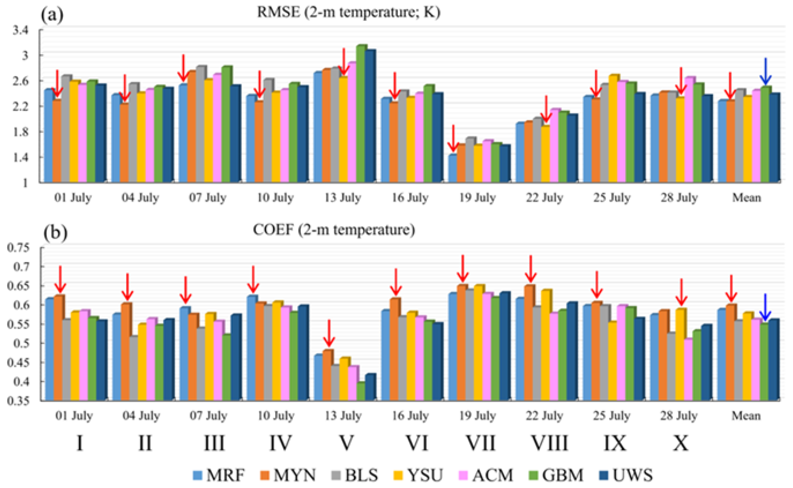
For the overall performance of the 2 m temperature forecast, as Figure 6a shows, the MYN scheme had the minimum RMSEs in five groups of runs (I, II, IV, VI, and IX), and those for the YSU scheme and the MRF scheme were three groups (V, VIII, and X) and two groups (III and VII), respectively. In terms of the COEF, the MYN scheme showed the maximum values in seven groups of runs (I, II, V, VI, VII, VIII, and IX; Figure 6b), and those for the MRF scheme and the YSU scheme were two groups (III and IV) and one group (X), respectively. For the mean state, the MYN scheme also showed the best performance, as it had the smallest RMSE and largest COEF (rightmost column of Figure 6), while the MRF scheme and YSU scheme ranked second and third, respectively.

3.3. Evaluation on 10 m Wind Forecast

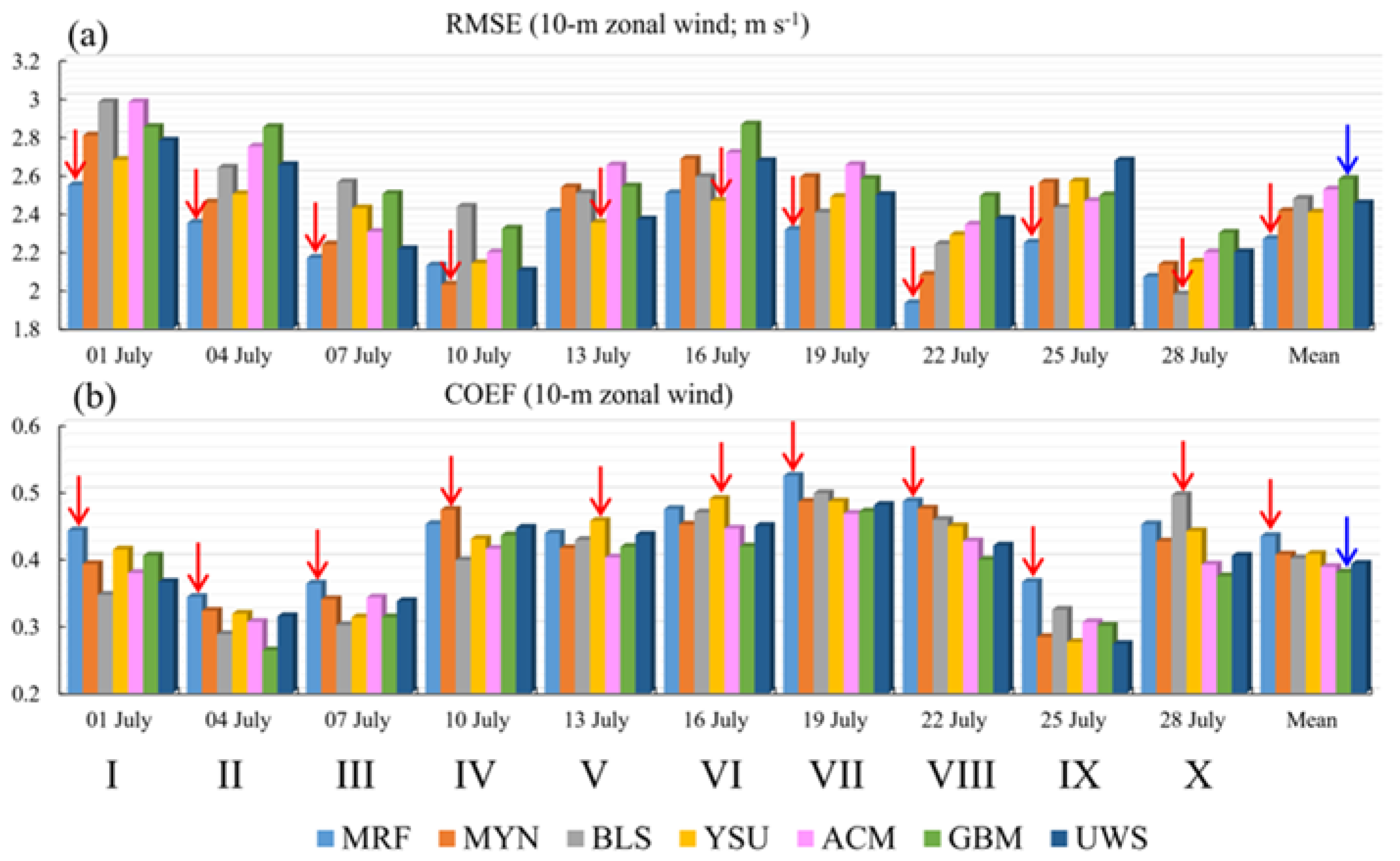
The power law is widely used to determine the wind speed at the 100 m hub height by using the 10 m wind speed [27,51]. This means that the 10 m wind speed is closely related to the 100 m wind speed; thus, it is also necessary to evaluate the forecast accuracy of the 10 m wind. From Figure 7, it can be found that for the 10 m zonal wind, the MRF scheme showed the overall best performance, because (i) it had the smallest RMSEs in six groups (I, II, III, VII, VIII, and IX) and the mean state, and (ii) it had the largest COEFs in six groups (I, II, III, VII, VIII, and IX) and the mean state. The MYN and YSU schemes showed similar performances in terms of the mean state, and they both ranked second.
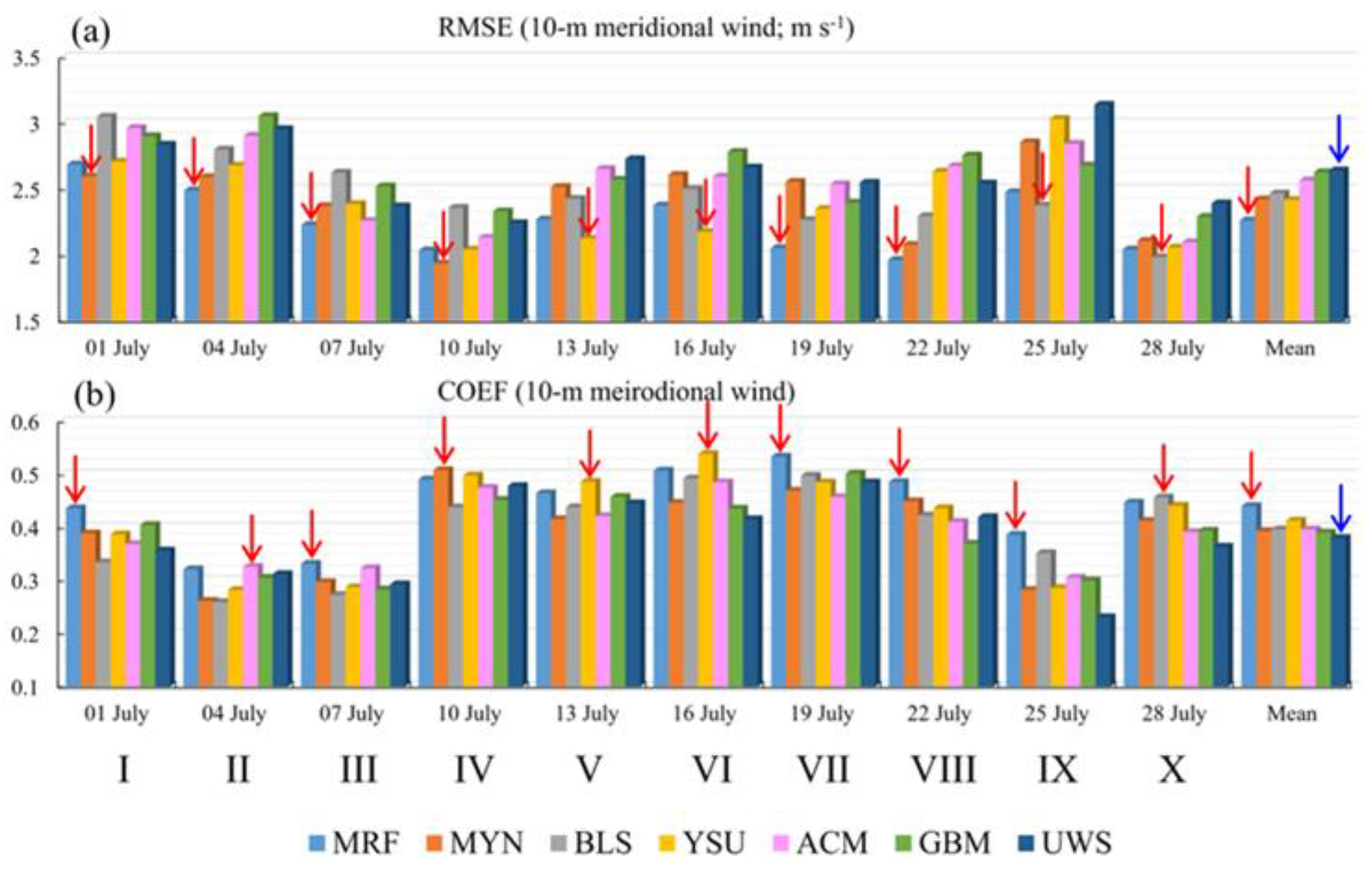
For the 10 m meridional wind, as Figure 8 shows, the MRF scheme also showed the best performance among all seven PBL schemes: its RMSEs were minimized in four groups of runs (II, III, VII, and VIII) and the mean state, and its COEFs were maximized in five groups of runs (I, III, VII, VIII, and IX) and the mean state. The YSU scheme was the second best scheme in terms of the mean state, and the MYN scheme ranked third.
In summary, as discussed in Section 3.1, Section 3.2 and Section 3.3, the MRF showed the overall best performance for forecasting the factors that were used for calculating the WPD. Therefore, as the shading in Figure 5 shows, the temporal mean (from 1 July to 31 July) of the WPD forecasted by the MRF showed the most consistent features with the WPD calculated by ERA5. Therefore, it is strongly recommended to use the MRF scheme for the WPD forecast in the middle- and high-latitude regions of China.

4. Evaluation on the Forecasts of the Background Conditions

4.1. Evaluation on 500 hPa Geopotential Height Forecast

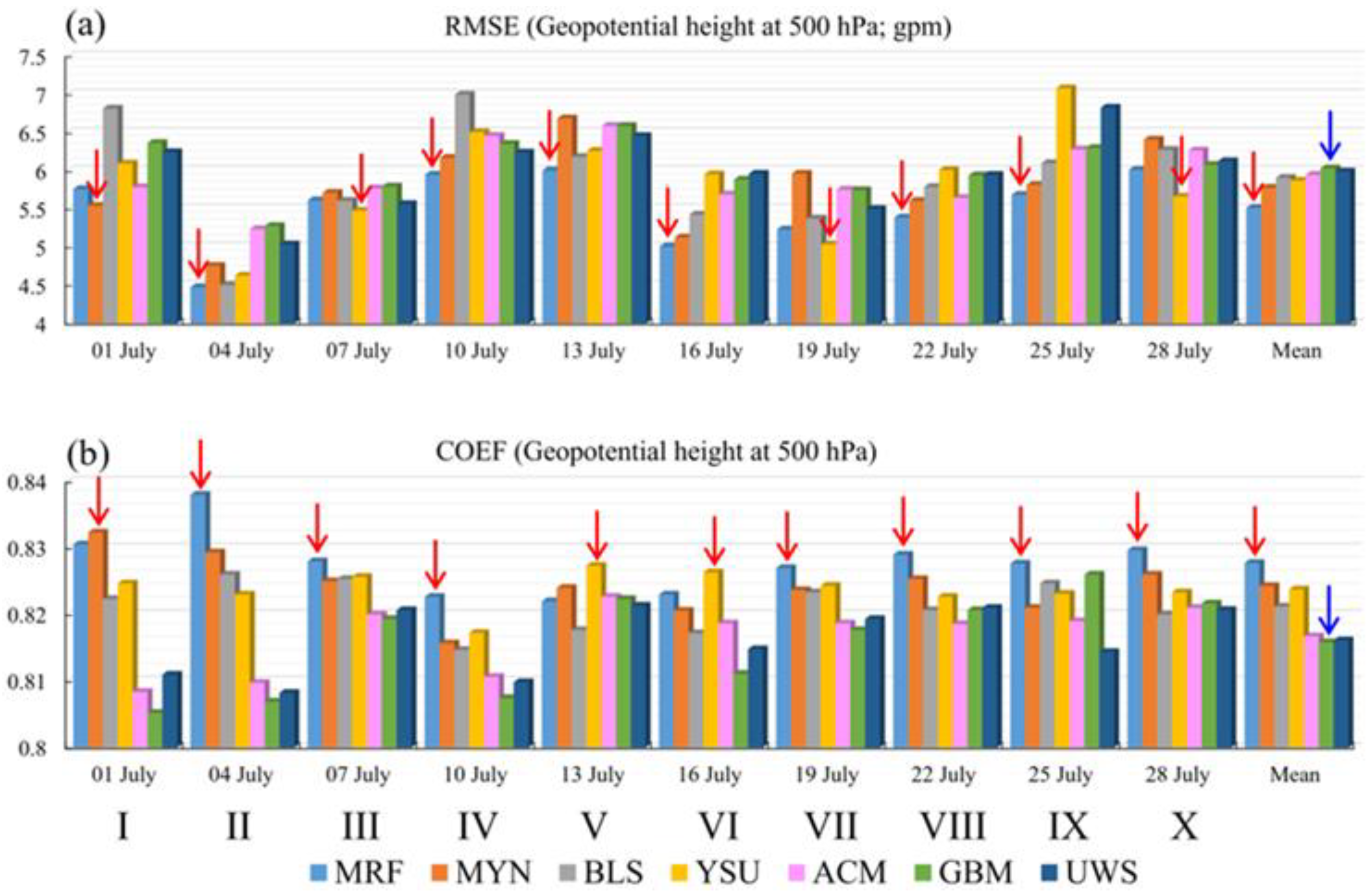
According to the quasi-geostrophic theory, the weather systems at 500 hPa (e.g., trough, ridge, cyclones, etc.) exert notable effects on the lower-level systems [7,25]. This could directly affect the 100 m wind field, and therefore, it is necessary to evaluate the forecast of 500 hPa geopotential height. From Figure 9, it can be found that the MRF was the best scheme because (i) it showed the smallest RMSEs in six groups of runs (II, IV, V, VI, VIII, and IX) and the mean state, and (ii) it showed the largest COEFs in seven groups (II, III, IV, VII, VIII, IX, and X) and the mean state. The MYN and YSU schemes ranked second and third, respectively, in terms of the mean state. This is consistent with the ranking of the 100 m wind speed forecast, as a better 500 hPa geopotential height forecast provided better background conditions for the weather systems at lower levels. The temporal mean (from 1 July to 31 July) of the 500 hPa geopotential height is shown in Figure 10. We found that the shortwave trough that appeared in the regions east of 108° E reproduced by the MRF scheme was the most consistent with that of ERA5. Moreover, for this scheme, the 500 hPa temperature field and 200 hPa strong wind band were also well forecasted. All these contributed to a high-skill forecast of the 100 m wind speed.

4.2. Evaluation on the 24-h Accumulated Precipitation Forecast

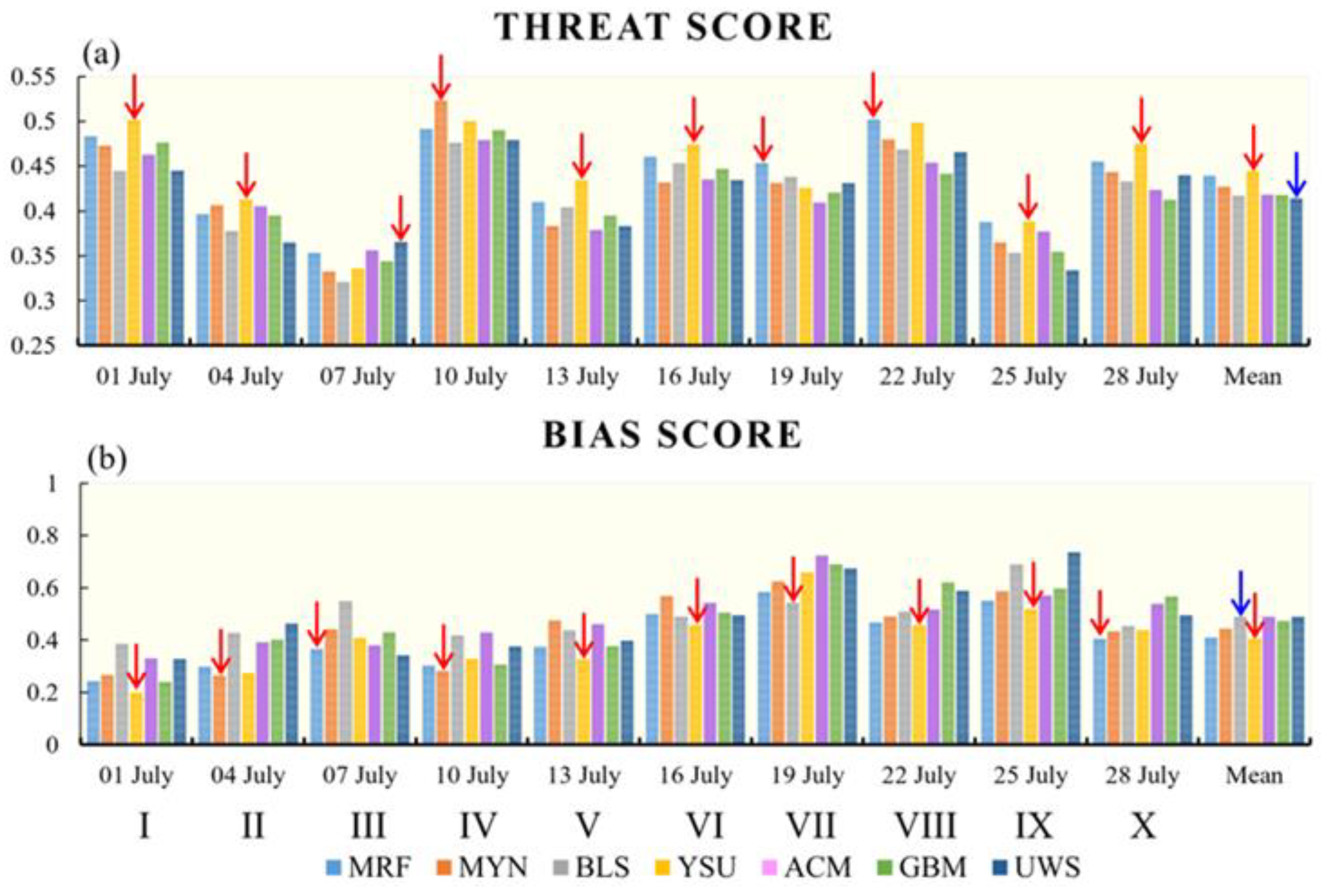
Precipitation is the product of the evolution of weather systems, and it can feed back on the weather systems through releasing latent heat. The greater the intensity of the precipitation, the stronger the feedback. For precipitation no weaker than moderate rain (i.e., 24 h precipitation ≥ 10 mm), the overall performances of different PBL schemes are illustrated in Figure 11. We found that in terms of the threat score (Figure 11a), the YSU scheme showed the highest forecast skill, as its TS was the largest for six groups of runs (I, II, V, VI, IX, and X) and the mean state. The MRF and MYN schemes ranked second and third, respectively, in terms of the mean state. For the BIAS score, as Figure 11b shows, the YSU was also the best scheme, as its BIAS was the smallest for five groups of runs (I, V, VI, VIII, and IX) and the mean state. In terms of the mean state of BIAS, the MRF and MYN schemes also ranked second and third, respectively. In summary, as mentioned above, for the 24 h precipitation forecast, the YSU, MRF, and MYN schemes ranked first to third, respectively (Table 2).
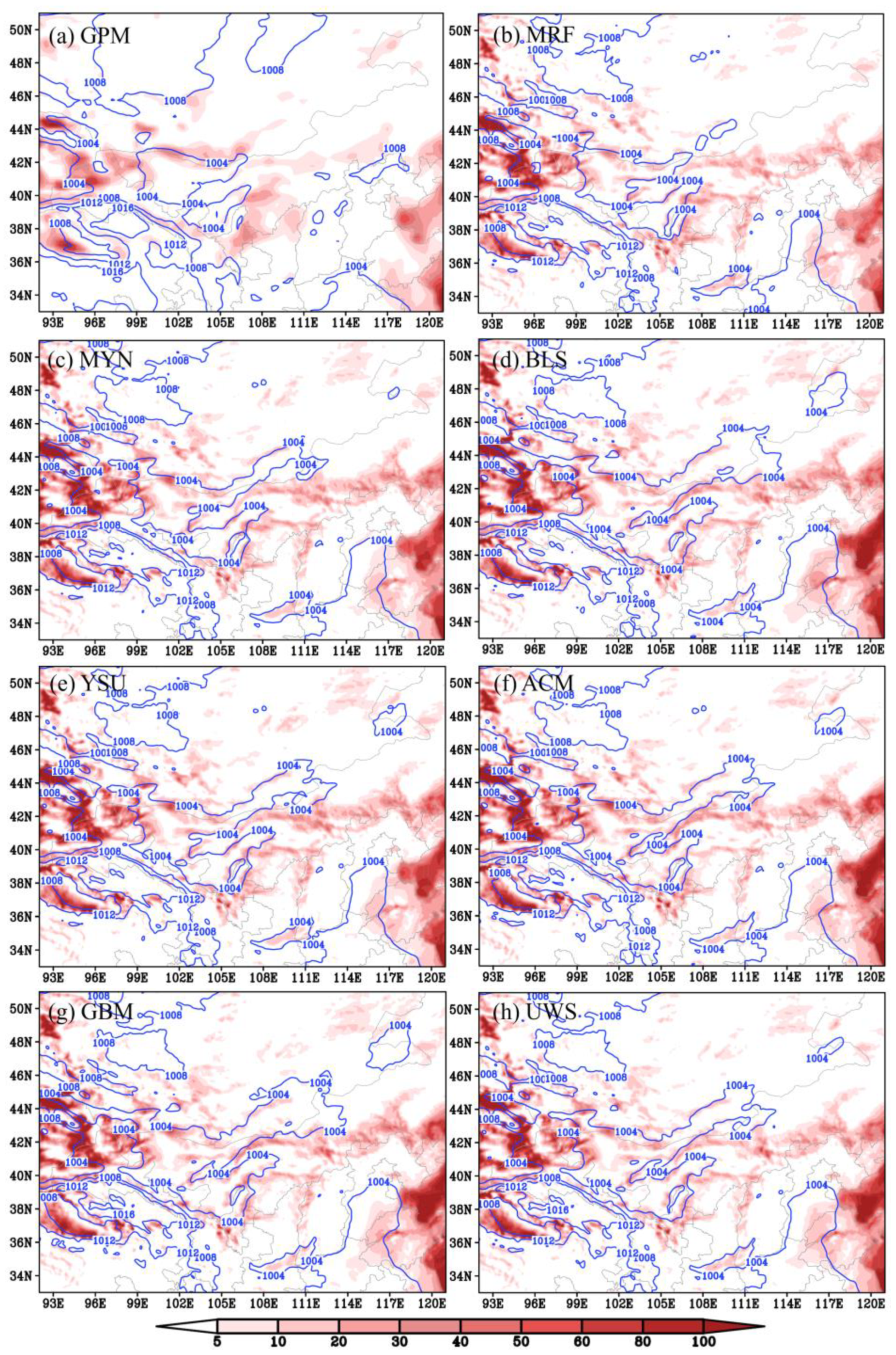
The accumulated precipitation of July is illustrated in Figure 12. It can be seen that there were mainly four precipitation centers in July 2021 (numbers in Figure 12a). All seven PBL schemes overestimated the precipitation centers I–IV, with the smallest overestimation in YSU (Figure 12e). This also confirmed that the precipitation was reproduced the best by the YSU scheme. Compared with others, the overestimations of the precipitation forecast were smaller in the runs with MRF and MYN. For the precipitation intensity of heavy rainfall (i.e., 24 h accumulated precipitation was between 25 mm and 49.9 mm) and torrential rainfall (i.e., 24 h accumulated precipitation was above 50 mm), MRF and YSU ranked first and second (not shown). This also explained why the four precipitation centers were well reproduced by these two PBL schemes. In July 2021, the PBL was frequently unstable (rainfall was frequent), and therefore, the MRF scheme showed an overall better performance than the other PBL schemes, as it allowed a more accurate description of deeper mixing in an unstable PBL [33]. A better precipitation forecast acted as a favorable background condition for the 100 m wind speed forecast.

5. Conclusions and Discussion

Of all the current power generation technologies, wind power generation shows the lowest carbon emissions. Therefore, to reach the goal of carbon neutralization, wind power generation plays an indispensable role. However, due to the randomness, diversity, intermittence, and uncontrollability of wind at near-surface levels, accurately forecasting the WPD on wind farms is still challenging. As the wind turbines of wind farms are situated in the PBL, where the turbulence, sensible heat flux, latent heat flux, and friction dissipation all exert direct effects on the near-surface wind field, it is crucial to select the relatively optimal PBL scheme to improve the WPD forecast. The middle- and high-latitude regions of China have the most abundant wind energy resources in China. Improving the wind power density forecast in this region is of particular importance to China’s wind power industry. In view of this, we compared the performances of seven PBL schemes (i.e., MRF, MYN, BLS, YSU, ACM, GBM, and UWS) by using the WRF model v4.4 for a total of 70 runs (for each run, the forecast period was 3 days). Overall, for all evaluations, we found that (i) there were no PBL schemes which could always show the best performances in forecasting all variables; (ii) the forecasts mainly became worse as the forecast time grew; and (iii) the forecast accuracy showed a notable dependence on the evolution of the weather systems. For some types of weather systems (e.g., high-pressure ridge, anticyclone, etc.) or during some stages of a weather system (e.g., slowly varying stage, steady maintain stage, etc.), the forecast accuracy was relatively high, whereas for others, the accuracy was lower. How the forecast accuracy depends on the weather systems’ evolution is an important scientific question which deserves further investigation.
To evaluate the forecast accuracy of the WPD, according to its calculation expression, we evaluated a total of three factors: the first was the 100 m wind speed, which played a decisive role in calculating the WPD; the second and the third were the sea level pressure and 2 m temperature, both of which not only could reflect the forecast accuracy of the air density, but also could affect the evolution of the 100 m wind speed through pressure gradient force and baroclinity (stronger baroclinity was favorable for more intense release of the available potential energy, during which the kinetic energy would be enhanced). In terms of the evaluation of the 100 m wind speed, it was found that for the 24 h, 48 h, and 72 h forecasts and their total, the MRF scheme was the best (Table 1), whereas the GBM scheme showed the lowest forecast skills among all seven PBL schemes. For the forecast of the sea level pressure, the MRF scheme also showed the best performance, whereas for the 2 m temperature forecast, the MYN scheme ranked first, and the MRF scheme ranked second. Therefore, we strongly recommend using the MRF scheme for the WPD forecast in the middle- and high-latitude regions of China.
In addition to the WPD forecast, the MRF scheme also showed the best performances when forecasting the 10 m zonal wind, 10 m meridional wind, and 500 hPa geopotential height. For precipitation no weaker than moderate rainfall, the MRF scheme ranked second, while the YSU scheme ranked first (Table 2). Overall, these findings indicate that the background conditions for the evolution of the 100 m wind speed were well forecasted by the MRF scheme, which contributed to obtaining a relatively optimal WPD forecast. However, as we only used one month in the summer (July 2021) to evaluate the performances of different PBL schemes, whether the results could be suitable for other seasons still needs further comparison. Moreover, in addition to the PBL schemes, the microphysics schemes also notably affect the forecast accuracy of the WPD. Therefore, we suggest conducting the evaluations on different microphysics schemes, and the WPD forecast in the middle- and high-latitude regions of China could thus be further improved.

Author Contributions

Conceptualization, H.M. and X.C.; methodology, X.M.; software, H.S.; validation, H.M., X.C. and Y.J.; formal analysis, H.M. and X.C.; investigation, H.M., X.C., H.S. and K.Z.; resources, H.S.; data curation, Y.J.; writing—original draft preparation, H.M.; writing—review and editing, H.M. and X.C.; visualization, X.M.; supervision, X.C.; project administration, H.M.; funding acquisition, X.C. All authors have read and agreed to the published version of the manuscript.

Funding

This research was supported by the Key Research and Development Program of Hebei Province (grant no. 21314303D).

Institutional Review Board Statement

Not applicable.

Informed Consent Statement

Not applicable.

Data Availability Statement

Not applicable.

Acknowledgments

The authors sincerely thank the China Meteorological Administration for providing the surface observational data; we also would like to thank the ECMWF and NASA for providing the 10-day forecast, the ERA5 reanalysis, and the GPM precipitation data.

Conflicts of Interest

The authors declare no conflict of interest.

References

  1. Fu, S.M.; Yu, F.; Wang, D.H.; Xia, R.D. A comparison of two kinds of eastward-moving mesoscale vortices during the mei-yu period of 2010. Sci. China Earth Sci. 2013, 56, 282–300. [Google Scholar] [CrossRef]
  2. Fu, S.M.; Liu, R.X.; Sun, J.H. On the scale interactions that dominate the maintenance of a persistent heavy rainfall event: A piecewise energy analysis. J. Atmos. Sci. 2018, 75, 907–925. [Google Scholar] [CrossRef]
  3. Li, R.S. Distributed Power Resources: Operation and Control of Connecting to the Grid; Academic Press: New York, NY, USA, 2019; 248p. [Google Scholar] [CrossRef]
  4. Schlömer, S.; Bruckner, T.; Fulton, L.; Hertwich, E.; McKinnon, A.; Perczyk, D.; Roy, J.; Schaeffer, R.; Sims, R.; Smith, P.; et al. Annex III: Technology-specific cost and performance parameters. In Climate Change 2014: Mitigation of Climate Change. Contribution of Working Group III to the Fifth Assessment Report of the Intergovernmental Panel on Climate Change; Cambridge University Press: Cambridge, UK; New York, NY, USA, 2014; Volume 133. [Google Scholar]
  5. Fu, S.M.; Mai, Z.; Sun, J.H.; Li, W.L.; Zhong, Q.; Sun, J.R.; Zhang, Y.C. A semi-idealized modeling study on the long-lived eastward propagating mesoscale convective system over the Tibetan Plateau. Sci. China Earth Sci. 2021, 64, 1996–2014. [Google Scholar] [CrossRef]
  6. Calif, R.; Schmitt, F.G.; Huang, Y. Multifractal description of wind power fluctuations using arbitrary order Hilbert spectral analysis. Phys. A Stat. Mech. Its Appl. 2013, 392, 4106–4120. [Google Scholar] [CrossRef]
  7. Fu, S.M.; Jin, S.L.; Shen, W.; Li, D.Y.; Liu, B.; Sun, J.H. A kinetic energy budget on the severe wind production that cause a serious state grid failure in Southern Xinjiang China. Atmos. Sci. Lett. 2020, 2020, e977. [Google Scholar] [CrossRef]
  8. Jin, S.L.; Feng, S.L.; Shen, W.; Fu, S.M.; Jiang, L.Z.; Sun, J.H. Energetics characteristics accounting for the low-level wind’s rapid enhancement associated with an extreme explosive extratropical cyclone over the western North Pacific Ocean. Atmos. Ocean. Sci. Lett. 2020, 13, 426–435. [Google Scholar] [CrossRef]
  9. Ahmad, T.; Zhang, D. A data-driven deep sequence-to-sequence long-short memory method along with a gated recurrent neural network for wind power forecasting. Energy 2022, 239, 122109. [Google Scholar] [CrossRef]
  10. Wu, C.; Luo, K.; Wang, Q.; Fan, J. Simulated potential wind power sensitivity to the planetary boundary layer parameterizations combined with various topography datasets in the weather research and forecasting model. Energy 2022, 239, 122047. [Google Scholar] [CrossRef]
  11. Howard, T.; Clark, P. Correction and downscaling of NWP wind speed forecasts. Meteorol. Appl. 2007, 14, 105–116. [Google Scholar] [CrossRef]
  12. Ma, H.; Ma, X.; Mei, S.; Wang, F.; Jing, Y. Improving the Near-Surface Wind Forecast around the Turpan Basin of the Northwest China by Using the WRF_TopoWind Model. Atmosphere 2021, 12, 1624. [Google Scholar] [CrossRef]
  13. Jin, S.L.; Feng, S.L.; Wang, B.; Liu, X.L.; Hu, J.; Song, Z.P. Applicability of Planetary Boundary Layer Parameterization Schemes for Wind Field Numerical Prediction in China Northwest Power Grid. High Volt. Eng. 2022, 48, 435–447. [Google Scholar]
  14. Liu, H.; Mi, X.W.; Li, Y.F. Smart wind speed deep learning based multi-step forecasting model using singular spectrum analysis, convolutional gated recurrent unit network and support vector regression. Renew. Energy 2019, 143, 842–854. [Google Scholar] [CrossRef]
  15. Harbola, S.; Coors, V. One dimensional convolutional neural network architectures for wind prediction. Energy Convers. Manag. 2019, 195, 70–75. [Google Scholar] [CrossRef]
  16. Moreno, S.R.; Silva, R.G.D.; Mariani, V.C. Multi-step wind speed forecasting based on hybrid multi-stage decomposition model and long short-term memory neural network. Energy Convers. Manag. 2020, 213, 112869. [Google Scholar] [CrossRef]
  17. Wang, T.; Ma, S.; Gao, Y.; Gong, Y.; An, Z. The hybrid of wavelet packet decomposition and machine learning models in wind speed forecasting. J. Desert Res. 2021, 41, 38–50. [Google Scholar]
  18. Bai, Y.; Fang, D.; Hou, Y. Regional wind power forecasting system for Inner Mongolia power grid. Power Syst. Technol. 2010, 34, 157–162. [Google Scholar]
  19. Zhang, H.; Sun, K.; Tian, L.; Yan, G. Wind speed simulation of wind farm using WRF model. J. Tianjin Univ. 2012, 45, 1116–1120. [Google Scholar]
  20. Skamarock, W.C.; Klemp, J.B.; Dudhia, J.; Gill, D.O.; Barker, D.M.; Duda, M.G.; Huang, X.Y.; Wang, W.; Powers, J.G. A Description of the Advanced Research WRF Version 3. NCAR Tech. Note CAR/TN-475+STR, 113. 2008. Available online: https://opensky.ucar.edu/islandora/object/technotes:500 (accessed on 1 May 2022).
  21. Han, C.; Nan, M. Application and analysis of the wind resource assessment with WAsP software. Energy Eng. 2009, 4, 26–30. [Google Scholar]
  22. Frank, H.P.; Rathmann, O.; Mortensen, N.G.; Landberg, L. The Numerical Wind Atlas—The KAMM/WAsP Method; Risoe-R No. 1252; Forskningscenter Risoe: Roskilde, Denmark, 2001. [Google Scholar]
  23. Shikhovtsev, A.; Kovadlo, P.; Lukin, V.; Nosov, V.; Kiselev, A.; Kolobov, D.; Kopylov, E.; Shikhovtsev, M.; Avdeev, F. Statistics of the Optical Turbulence from the Micrometeorological Measurements at the Baykal Astrophysical Observatory Site. Atmosphere 2019, 10, 661. [Google Scholar] [CrossRef] [Green Version]
  24. Shikhovtsev, A.; Kovadlo, P.; Kiselev, A. Astroclimatic statistics at the Sayan Solar Observatory. Solar-Terr. Phys. 2020, 6, 102–107. [Google Scholar] [CrossRef]
  25. Holton, J.R. An Introduction to Dynamic Meteorology; Academic Press: San Diego, CA, USA, 2004. [Google Scholar]
  26. Yang, M.; Patiño-Echeverri, D.; Yang, F. Wind power generation in China: Understanding the mismatch between capacity and generation. Renew. Energy 2012, 41, 145–151. [Google Scholar] [CrossRef]
  27. Li, M.; Shen, Y.; Yao, J.; Ye, D.; Fan, J.; Simmonds, I. An assessment of observed wind speed and wind power density over China for 1980–2021. Wind Energy 2022, 1–25. [Google Scholar] [CrossRef]
  28. Yang, P.; Wang, X.; Wang, L.; Zhu, Y. A study on the applicability of WRF_TopoWind model to simulate the mountain wind speed of the low latitude plateau in China. J. Yunnan Univ. Nat. Sci. Ed. 2016, 38, 766–772. [Google Scholar]
  29. Mughal, M.O.; Lynch, M.; Yu, F.; McGann, B.; Jeanneret, F.; Sutton, J. Wind modelling, validation and sensitivity study using Weather Research and Forecasting model in complex terrain. Environ. Model. Softw. 2017, 90, 107–125. [Google Scholar] [CrossRef]
  30. Salvaçao, N.; Soares, C.G. Wind resource assessment offshore the Atlantic Iberian coast with the WRF model. Energy 2018, 145, 276–287. [Google Scholar] [CrossRef]
  31. Prosper, M.A.; Otero-Casal, C.; Canoura, F.F.; Miguez-Macho, G. Wind power forecasting for a real onshore wind farm on complex terrain using WRF high resolution simulations. Renew. Energy 2019, 135, 674–686. [Google Scholar] [CrossRef]
  32. Huffman, G.J.; Stocker, E.F.; Bolvin, D.T.; Nelkin, E.J.; Tan, J. GPM IMERG Final Precipitation L3 1 Day 0.1 Degree x 0.1 Degree V06; Savtchenko, A., Ed.; Goddard Earth Sciences Data and Information Services Center (GES DISC): Greenbelt, MD, USA, 2019. [CrossRef]
  33. Hong, S.; Pan, H. Nonlocal boundary layer vertical diffusion in a medium range forecast model. Mon. Weather Rev. 1996, 124, 2322–2339. [Google Scholar] [CrossRef]
  34. Mlawer, E.J.; Taubnam, S.J.; Brown, P.D.; Iacono, M.J.; Clough, S.A. Radiative transfer for inhomogeneous atmospheres: RRTM, a validated correlated-k model for the longwave. J. Geophys. Res. 1997, 102, 16663–16682. [Google Scholar] [CrossRef] [Green Version]
  35. Dudhia, J. Numerical Study of Convection Observed during the Winter Monsoon Experiment Using a Mesoscale Two-Dimensional Model. J. Atmos. Sci. 1989, 46, 3077–3107. [Google Scholar] [CrossRef]
  36. Chen, F.; Dudhia, J. Coupling an advanced landsurface hydrology model with the Penn State/NCAR MM5 modeling system. Part I: Model description and implementation. Mon. Weather Rev. 2001, 129, 569–585. [Google Scholar] [CrossRef]
  37. Huang, L.; Luo, Y.; Bai, L. An evaluation of convection-permitting ensemble simulations of coastal nocturnal rainfall over South China during the early-summer rainy season. J. Geophys. Res. Atmos. 2022, 127, e2021JD035656. [Google Scholar] [CrossRef]
  38. Nakanishi, M.; Niino, H. An improved Mellor–Yamada level-3 model with condensation physics: Its design and verification. Bound.-Layer Meteorolol. 2004, 112, 1–31. [Google Scholar] [CrossRef]
  39. Bougeault, P.; Lacarrere, P. Parameterization of orography-induced turbulence in a mesobeta-scale model. Mon. Weather Rev. 1989, 117, 1872–1890. [Google Scholar] [CrossRef]
  40. Hong, S.; Noh, Y. A New Vertical diffusion package with an explicit treatment of entrainment processes. Mon. Weather Rev. 2006, 134, 2318–2341. [Google Scholar] [CrossRef]
  41. Pleim, J. A combined local and nonlocal closure model for the atmospheric 611 boundary layer. Part I: Model description and testing. J. Appl. Meteorol. Climatol. 2007, 46, 1383–1395. [Google Scholar] [CrossRef]
  42. Grenier, H.; Bretherton, C. A moist PBL parameterization for large-scale models and its application to subtropical cloud-topped marine boundary layers. Mon. Weather Rev. 2001, 129, 357–377. [Google Scholar] [CrossRef]
  43. Bretherton, C.; Sungsu, P. A New Moist Turbulence Parameterization in the Community Atmosphere Model. J. Clim. 2009, 22, 3422–3448. [Google Scholar] [CrossRef]
  44. Fu, S.M.; Zhang, Y.C.; Wang, H.J.; Tang, H.; Li, W.L.; Sun, J.H. On the evolution of a long-lived mesoscale convective vortex that acted as a crucial condition for the extremely strong hourly precipitation in Zhengzhou. J. Geophys. Res. Atmos. 2022, 127, e2021JD036233. [Google Scholar] [CrossRef]
  45. Fu, S.M.; Mai, Z.; Sun, J.H.; Li, W.L.; Ding, D.; Wang, Y.Q. Impacts of convective activity over the Tibetan Plateau on plateau vortex, southwest vortex, and downstream precipitation. J. Atmos. Sci. 2019, 76, 3803–3830. [Google Scholar] [CrossRef]
  46. Etherton, B.; Santos, P. Sensitivity of WRF forecasts for South Florida to initial conditions. Weather Forecast. 2008, 23, 725–740. [Google Scholar] [CrossRef] [Green Version]
  47. Kong, F.; Xue, M.; Thomas, K. Real-time storm-scale ensemble forecast experiment -analysis of 2008 spring experiment data. In Proceedings of the 24th Conference on Several Local Storms, Savannah, GA, USA, 27–31 October 2008; American Meteorological Society: Boston, MA, USA, 2008. [Google Scholar]
  48. Gualtieri, G. Reliability of ERA5 reanalysis data for wind resource assessment: A comparison against tall towers. Energies 2021, 14, 4169. [Google Scholar] [CrossRef]
  49. Aboobacker, V.M.; Shanas, P.R.; Veerasingam, S.; Al-Ansari, E.M.A.S.; Sadooni, F.N.; Vethamony, P. Long-term assessment of onshore and offshore wind energy potentials of Qatar. Energies 2021, 14, 1178. [Google Scholar] [CrossRef]
  50. Wen, Y.; Kamranzad, B.; Lin, P.Z. Assessment of long-term offshore wind energy potential in the south and southeast coasts of China based on a 55-year dataset. Energy 2021, 224, 120225. [Google Scholar] [CrossRef]
  51. Jung, C.; Schindler, D. The annual cycle and intra-annual variability of the global wind power distribution estimated by the system of wind speed distributions. Sustain. Energy Technol. Assess. 2020, 42, 100852. [Google Scholar] [CrossRef]
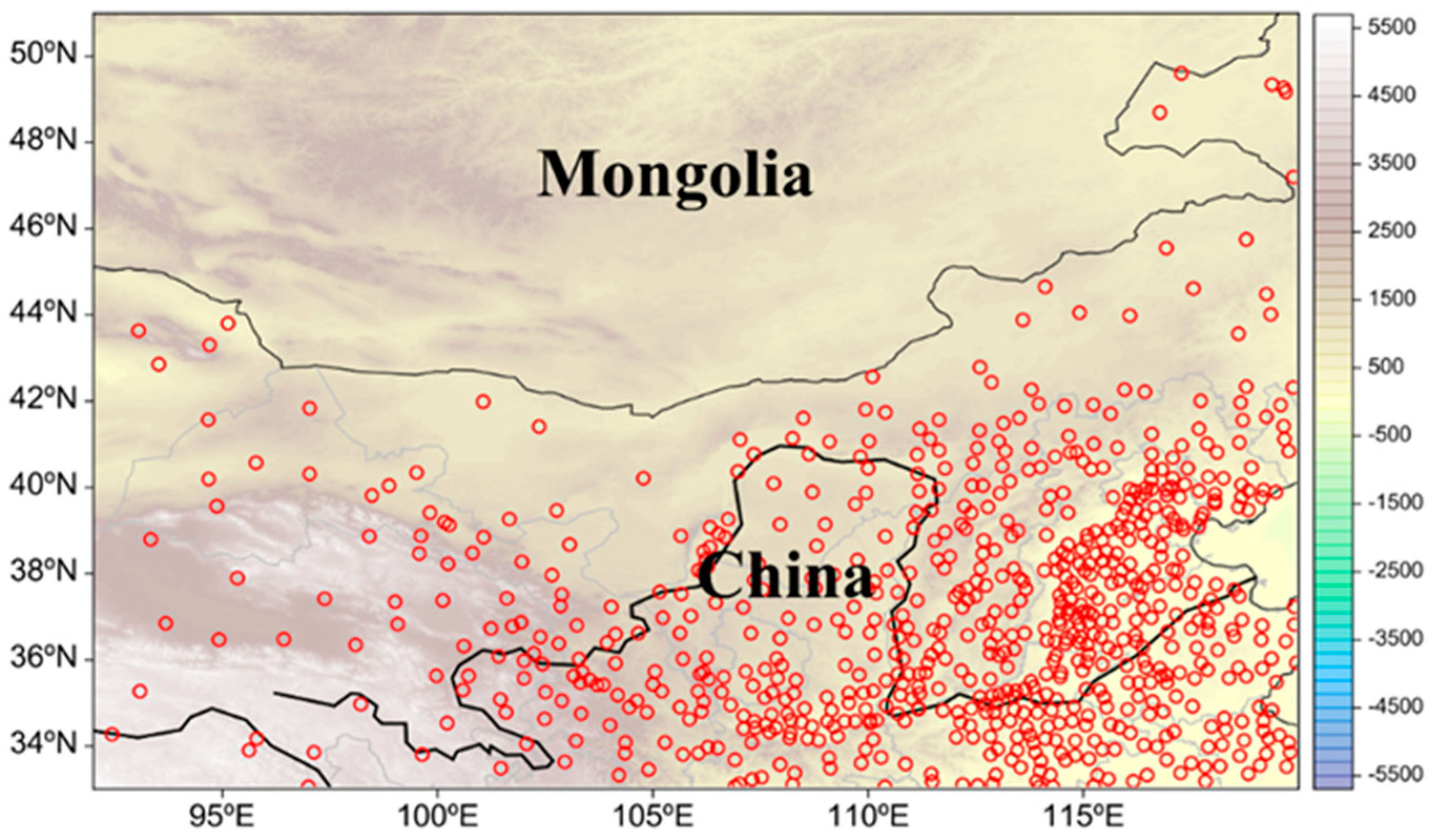
Figure 1. Distribution of the surface observational stations (small red circles) that were used for the evaluation of the performances of different PBL schemes, where the shading represents the terrain (m).
Atmosphere 13 02034 g001
Figure 2. The domain used for the simulations (the whole range was used in simulations), where the shading is the terrain (m).
Atmosphere 13 02034 g002
Figure 3. Panel (a) shows the correlation coefficient (COEF) for the 24 h forecast of the 100 m wind speed, and panel (b) shows the root mean square error (RMSE) for the 24 h forecast of the 100 m wind speed (b). Panel (c) is the same as (a) but for the 48 h forecast, and panel (d) is the same as (b) but for the 48 h forecast. Panel (e) is the same as (a) but for the 72 h forecast, and panel (f) is the same as (b) but for the 72 h forecast. The red arrow shows the best scheme, and the blue arrow marks the worst scheme. Mean = the temporal mean of all 10 runs from I to X.
Atmosphere 13 02034 g003
Figure 4. Panel (a) shows the averaged root mean square error (RMSE) for the 24 h, 48 h, and 36 h forecasts of the sea level pressure (hPa), and panel (b) shows the averaged correlation coefficient (COEF) for the 24 h, 48 h, and 36 h forecasts of the sea level pressure, where the red arrow shows the best scheme, the small shaded boxes mark the overall best scheme, and the blue arrow marks the worst scheme. Mean = the temporal mean of all 10 runs from 1 July to 28 July.
Atmosphere 13 02034 g004
Figure 5. Panel (a) shows the temporal mean (from 1 July to 31 July) of the sea level pressure (blue contour; hPa) and the wind power intensity at the height of 100 m (shading; W m−2). Panel (b) is the same as (a) but for the simulation using the MRF scheme. Panel (c) is the same as (b), but for the MYN scheme. Panel (d) is the same as (b), but for the BLS scheme. Panel (e) is the same as (b), but for the YSU scheme. Panel (f) is the same as (b), but for the ACM scheme. Panel (g) is the same as (b), but for the GBM scheme. Panel (h) is the same as (b), but for the UWS scheme.
Atmosphere 13 02034 g005
Figure 6. Panel (a) shows the averaged root mean square error (RMSE) for the 24 h, 48 h, and 36 h forecasts of the 2 m temperature (K), and panel (b) shows the averaged correlation coefficient (COEF) for the 24 h, 48 h, and 36 h forecasts of the 2 m temperature, where the red arrow shows the best scheme, and the blue arrow marks the worst scheme. Mean = the temporal mean of all 10 runs from 1 July to 28 July.
Atmosphere 13 02034 g006
Figure 7. Panel (a) shows the averaged root mean square error (RMSE) for the 24 h, 48 h, and 36 h forecasts of the 10 m zonal wind (m s−1), and panel (b) shows the averaged correlation coefficient (COEF) for the 24 h, 48 h, and 36 h forecasts of the 10 m zonal wind, where the red arrow shows the best scheme, and the blue arrow marks the worst scheme. Mean = the temporal mean of all 10 runs from 1 July to 28 July.
Atmosphere 13 02034 g007
Figure 8. Panel (a) shows the averaged root mean square error (RMSE) for the 24 h, 48 h, and 36 h forecasts of the 10 m meridional wind (m s−1), and panel (b) shows the averaged correlation coefficient (COEF) for the 24 h, 48 h, and 36 h forecasts of the 10 m meridional wind, where the red arrow shows the best scheme, and the blue arrow marks the worst scheme. Mean = the temporal mean of all 10 runs from 1 July to 28 July.
Atmosphere 13 02034 g008
Figure 9. Panel (a) shows the averaged root mean square error (RMSE) for the 24 h, 48 h, and 36 h forecasts of the 500 hPa geopotential height (gpm), and panel (b) shows the averaged correlation coefficient (COEF) for the 24 h, 48 h, and 36 h forecasts of the 500 hPa geopotential height, where the red arrow shows the best scheme, and the blue arrow marks the worst scheme. Mean = the temporal mean of all 10 runs from 1 July to 28 July.
Atmosphere 13 02034 g009
Figure 10. Panel (a) shows the temporal mean (from 1 July to 31 July) of the 500 hPa geopotential height (black contour; gpm), the 500 hPa temperature (red contour; °C), and the 200 hPa strong wind (shading; m s−1). Panel (b) is the same as (a) but for the simulation using the MRF scheme. Panel (c) is the same as (b), but for the MYN scheme. Panel (d) is the same as (b), but for the BLS scheme. Panel (e) is the same as (b), but for the YSU scheme. Panel (f) is the same as (b), but for the ACM scheme. Panel (g) is the same as (b), but for the GBM scheme. Panel (h) is the same as (b), but for the UWS scheme.
Atmosphere 13 02034 g010
Figure 11. Panel (a) shows the averaged threat score for the 24 h, 48 h, and 36 h forecasts of 24 h accumulated precipitation, and panel (b) shows averaged bias score for the 24 h, 48 h, and 36 h forecasts of 24 h accumulated precipitation, where the red arrow shows the best scheme, and the blue arrow marks the worst scheme. Mean = the temporal mean of all 10 runs from 1 July to 28 July.
Atmosphere 13 02034 g011
Figure 12. Panel (a) shows the accumulated precipitation from 1 July to 31 July (shading; mm) derived from the GPM precipitation. Panel (b) is the same as (a) but for the simulation using the MRF scheme. Panel (c) is the same as (b), but for the MYN scheme. Panel (d) is the same as (b), but for the BLS scheme. Panel (e) is the same as (b), but for the YSU scheme. Panel (f) is the same as (b), but for the ACM scheme. Panel (g) is the same as (b), but for the GBM scheme. Panel (h) is the same as (b), but for the UWS scheme. ‘I’, ‘II’, ‘III’, and ‘IV’ mark the four precipitation centers.
Atmosphere 13 02034 g012
Table 1. A summary of the planetary boundary layer schemes used in this study, where ‘Local’ means that for a given point, only the points directly vertically adjacent to it can affect it, and ‘Nonlocal’ means that for a given point, the points at multiple vertical levels can affect it.
Full NameAbbreviationKey FeaturesReference
The Medium-Range Forecast schemeMRFNonlocal[33]
The Mellor–Yamada Nakanishi and Niino Level 2.5 schemeMYNLocal[38]
The Bougeault and Lacarrere schemeBLSLocal[39]
The Yonsei University schemeYSUNonlocal[40]
The asymmetric convective model, version 2ACMNonlocal[41]
The Grenier–Bretherthon–McCaa
scheme
GBMLocal[42]
The University of Washington moist
turbulence scheme
UWSLocal[43]
Table 2. The schemes ranked from first to third in terms of the overall performance (i.e., the mean of the 24 h, 48 h, and 72 h forecasts).
Ranks FirstRanks SecondRanks Third
100 m wind speedMRFMYNYSU
10 m zonal windMRFMYN/YSU--
10 m meridional windMRFYSUMYN
Sea level pressureMRFYSUMYN
500 hPa geopotential heightMRFMYNYSU
2 m temperatureMYNMRFYSU
24 h precipitation YSUMRFMYN
Publisher’s Note: MDPI stays neutral with regard to jurisdictional claims in published maps and institutional affiliations.