Extreme Value Analysis of NO_x Air Pollution in the Winter Seaport of Varna

Abstract

The work studies extreme pollution events and their return period in the winter seaport of Varna, providing information for decision-makers, government agencies and civil society on how the intensity of shipping traffic may impact the air pollution in the vicinity of the port. Extreme value analysis employing the Weibull distribution is applied to investigate air pollution and the probability of higher concentrations of oxides of nitrogen ($N{O}_x$) generated by ships while queuing in the winter seaport. Potential cleaning of the air pollution generated by the anchored ships is introduced to meet the acceptable level of air pollution concentrations in coastal zones. The employed ship pollution cleaning and overall ship service costs are minimised to satisfy cleaner environmental conditions. The developed approach is adopted to analyse the air pollution of a port without a monitoring system to control and prevent pollution and with limited information on ship traffic and air pollution.

1. Introduction

The emission sources related to seaports include warehouses, plants, offices, ships, cranes, vehicles and many others [1,2]. Air pollution evaluation accounts for all pollutants, which in many cases are in the vicinity of the ports, originating from the industrial activities in yards and factories, urban areas, highway traffic and ship accidents [3], where the environmental conditions [4,5] need to be accounted for. The present study focuses on analysing the nitrogen oxide air pollution in the seaport of Varna.

The widely discussed nitrogen oxides represent a family of seven compounds [6], and the Environmental Protection Agency (EPA) regulates only nitrogen dioxide ($N{O}_2$) because it is the most prevalent form of $N{O}_x$ in the atmosphere generated by human activities. $N{O}_2$ reacts in the atmosphere to form ozone ($O_3$) and acid rain.

Nitrogen dioxide is the primary source of nitrate aerosols and, upon inhalation, reaches the lungs and converts into nitrous and nitric acid. An exposure of 0.06 to 0.1 ppm of $N{O}_2$ for two years causes acute respiratory disease [7]. The current WHO guideline value is 10 μg/m³ (annual mean) and 25 μg/m³ (24 h mean) [8].

Shipping accounts for 18 to 30 per cent of the total nitrogen oxides [7], where the $N{O}_x$ formation occurs due to a mixture of 21 per cent oxygen and 78 per cent nitrogen under certain operating conditions in the ship’s main engine.

Today, the amount of $N{O}_x$ emitted by shipping is controlled by the requirements of Annex VI of MARPOL, Regulation 13 $N{O}_x$ Technical Code 2008 (resolution MEPC.177(58) as amended by resolution MEPC.251(66) [9]). There are three levels (tiers) of control depending on the ship’s construction date.

Ships operating in Emission Control Areas (ECAs) and constructed on or after the given dates shall comply with the Tier III $N{O}_x$ standard as follows: 1 January 2016 and operating in the North American ECA and the United States Caribbean Sea ECA; or 1 January 2021 and operating in the Baltic Sea ECA or the North Sea ECA. The winter seaport studied here does not belong to an emission control area.

Table 1. Levels norm for ${NO}_{\mathrm{x}}$ emissions from ships [9].

Tier	Ship Construction Date On or After	Total Weighted Cycle Emission Limit (g/kWh) n = Engine’s Rated Speed (rpm)
		n < 130	n = 130–1999	n ≥ 2000
I	1 January 2000	17.0	45.n(−0.2)	9.8
II	1 January 2011	14.4	44.n(−0.23)	7.7
III	1 January 2016	3.4	9.n(−0.2)	2.0

shows the cycle emission limit related to $N{O}_x$ [9]. Gas emissions of nitrogen oxides, sulphur dioxide and particulate matter also have a significant impact [10] by violating the air quality in the populated harbour areas [11] and on human health [12].

The first study of air emissions in a port is from 20 years ago, and the following ones until 2014 are summarised in [13], considering academic studies on shipping emissions in 34 ports (13 of them in Spain). The share of $N{O}_x$ of total port-city emissions varies between 8% (Brindisi) and 33% (Hong Kong) [13]. The total amount of $N{O}_x$ emissions in 2011 was the second largest after CO₂ at 400,000 tons. More than 80% of port emissions come from containerships and tankers, which is explained by a more significant number of port calls—about 75%. The high emissions of container ships are accompanied by a short stay in ports, which is precisely the opposite for bulk carriers.

Recently, observed data from this period have been analysed and published for other European port cities. Ramacher, et al. [14] performed analyses for Rostock (Germany), Riga (Latvia) and the urban agglomeration of Gdansk–Gdynia (Poland). The contribution of NO₂ from shipping to overall air quality is about 22%, 11% and 16% for the three ports, respectively. The shipping contribution to the port environment is significantly higher, 46%, 44% and 26%, respectively, but it should be noted that ports make up less than 1% of the total impact area.

Ramacher, et al. [15] analysed the contributions of traffic and shipping emissions to city-scale $N{O}_x$ and PM_2.5 exposure in Hamburg (Germany). In terms of population-weighted mean exposure (PWE) to $N{O}_2$, the shipping contribution is 13.9% and is 1.6 times lower than that of traffic, which is 22.7%.

The impact of in-port ship emissions on the $NO$ and $N{O}_2$ average concentrations is 35% and 15%, respectively, for the port of Calais (France), one of the busiest European ports [16].

The amount of air emissions depends on the phase of the ship voyage [17,18]. The levels of nitrogen oxides vary during the ship’s manoeuvring in port, and they are lower than those at full speed. That is true only when no selective catalytic reduction (SCR) system is installed. The emissions at manoeuvring show seasonality dependence, for example, increasing the number of ferry lines at some period during the year. Analysed correlations between $N{O}_x$ and $P{M}_{10 }$ emissions during manoeuvring and hoteling of commercial ships are unreliable due to the lack of a sufficient amount of data [19]. Among the factors, tonnes of goods, hours of hoteling phase and port calls, the last shows the best correlation.

The analysis of emissions from 28 ocean-going ships in 2017 in Shanghai port [20] showed that the use of lower sulphur content (0.1% m/m) in the Emission Control Area (ECA) significantly reduces $S{O}_x$ and $P{M}_{10 }$ emissions by up to 94.4% and 78.3%, respectively, compared to using 0.5% m/m sulphur content. Unfortunately, this results in almost no reduction in $N{O}_{x }$ emissions because the low sulphur fuel does not affect them. This suggests the importance of implementing the ECA regulations for the coastal nations.

The influence of ships’ crew and port pilots’ qualifications on the emission from ships during manoeuvring in port areas is considered in [21]—the study showed a possible emission reduction of 12.5% or even more. Similar reductions for $N{O}_x$ and $S{O}_{2 }$ emissions of 8.70% ± 2.10% and 11.74% ± 2.95%, respectively, at the hotelling phase can be achieved by shore power adoption at the port [22].

The modelling of the extreme values of air pollution is not a new approach. Roberts [23,24] reviewed extreme values statistics with air quality data applications in two parts. The first part presented the principles of extreme value statistics, and particular emphasis was placed on the second largest value and its relation to the most significant value. The more familiar and valuable asymptotic distributions and their uses were also discussed. The second part of the study presented applications of the theory of air quality data.

Some aspects of the current state of the problem are presented in [25]. The study includes an overview of the methods based on goodness-of-statistics and root mean square error (RMSE) for extreme value distribution (EVD) families: Gumbel distribution (Type I), Fréchet distribution (Type II) and Weibull distribution (Type III). The study compared three estimation methods usually used to approximate the values of parameters for simulated observations: method of moments (MOMs), maximum likelihood estimator (MLE), and maximum product of spacing (MPS). This study recommended the MPS method regardless of the sample size because it provides better estimates for the unknown parameters and the reliability function.

To model extreme values of daily air pollution of $O_3$ and $N{O}_x$ based on two monitoring sites in Munich, the generalised form of the extreme value distribution (GEV) and the Pareto distribution (PD) were used in [26]. The study applied logistic regression to model the concentration measures’ probability of exceeding the official air quality standard. For $O_3$ and $N{O}_2$, significant effects of the weather variables such as temperature, wind velocity and atmospheric humidity were found.

The study presented in [27] analysed the monitored data for daily maximum eight-hour ozone in the UK for the most recent decade (2010–2019) using the generalised Pareto distribution (GPD). As a result, it gives the overall probability of exceeding a given ozone threshold.

GEV and GPD were applied to investigate the pollutants’ behaviour in two urban regions in Brazil [28]. Although there was a difference in the distributions, they presented similar results. The probability of higher concentrations of $CO, NO,N{O}_2,P{M}_{10}$ and $P{M}_{2.5}$ were more frequent during the winter and $O_3$ during the summer.

Extreme value analysis was used for analysing air pollution in Istanbul based on data from two permanent stations for hourly measuring of $S{O}_2$ and $N{O}_2$ concentrations, [29] showing that the Gumbel’s Type I and Type II extreme value distributions represented the air quality data very well.

Particulate matter $P{M}_{10}$ is also the subject of a study employing extreme value in Asia. The study in Malaysia [30] presented the use of EVD of the two-parameter Gumbel, two and three-parameter Weibull, GEV, and two and three-parameter GPD on the maximum concentration of daily ${PM}_{10}$ data recorded in the years 2010–2012 in several country regions. The result showed that the GEV distribution best fit all monitoring stations’ daily maximum concentration for $P{M}_{10}$.

The daily $P{M}_{10}$ concentration data from 2008 to 2019 in Thailand were used to analyse the 24 h averages and daily maxima from several stations by GPD [31]. The MLE and the bootstrap method dealt with the parameter estimation in GPD. The study highlighted the challenging issues in the extreme value analysis to determine a threshold. One of the results of practical importance is that the northern region is most likely to encounter high exposure to $P{M}_{10}$.

Su, et al. [32] analysed the exposures of 15 different volatile organic compounds (VOC), such as benzene, toluene, ethylbenzene etc., measured in the frame of two surveys in the USA. Using the highest 5 and 10% measurements, the GEV, Gumbel, and Lognormal distributions fit each VOC. Health risks for individual VOCs and three VOC mixtures were estimated. This analysis shows that GEV can represent peak exposures of VOCs, which are neither normally nor lognormally distributed. The distribution will be helpful in impact and policy analyses to describe concentrations, exposures, and risks.

The data collection method is also of great importance in analysing air pollution. A common approach is to use the automatic identification system (AIS) [33,34].

Based on modern IT technologies [35], Delhi has developed an internet of things (IoT) system to collect, visualise, analyse, and model urban air quality from August 2018 to December 2018. The IoT sensing system consists of multiple sensors connected to a micro-controller that transmits the sensed data to an IoT cloud and collects data for carbon dioxide ($C{O}_2$), carbon monoxide ($CO$), methane ($C{H}_4$), $PM$, noise, temperature, relative humidity, latitude, and longitude. Three EVD models were considered, i.e., Gumbel, Fréchet, Weibull, and one central fitting distribution—Lognormal. The goodness-of-fit criteria indicated that the Gumbel distribution model is better suited for analysing and forecasting air quality in this region. The average forecast error is about 6%.

Space technologies are also used to analyse air quality, where the changes in the ship ${NO}_{\mathrm{x}}$ emissions over European seas in 2019–2020 recorded by the TROPOMI sensor [36] were analysed. The Tropospheric Monitoring Instrument (TROPOMI) is the satellite instrument on board the Copernicus Sentinel-5 Precursor satellite (http://www.tropomi.eu/, accessed on 10 October 2022). The instrument provides accurate and timely observations of vital atmospheric species. The analysis showed stronger (35–75%) and sharper (10–35%) shipping $N{O}_2$ signals compared to co-sampled measurements from Ozone Monitoring Instrument (OMI). It was proved that $N{O}_x$ emissions from ships reduced by 10–20% during 2020.

During 2020–2021 the $N{O}_x$ emissions of 1407 ocean-going vessels (OGVs) in the Belgian North Sea were measured by the sniffer sensor system on the Belgian coastguard aircraft [37]. Unfortunately, measurements have found that the targeted reductions in OGV for $N{O}_x$ Tier II emissions, at least for the southern part of the North Sea, have not been achieved.

Parallel to the direct measurement of air pollution, the Gaussian dispersion models have been used for modelling air pollution emission transport [38,39]. The model accounts for meteorological conditions [40,41,42] for some time and geographical locations. Recently the Gaussian model has been used to predict air pollution dispersion in a crowded port area [43,44]. The study developed safety calibration factors that can define the distance from the populated areas to the source of pollution located at the seaport where the arriving ships are queuing. The study presented in [45] identifies the most suitable berth terminal operation for ships, conditional on ships’ air pollution and the cost of terminal operations.

The air quality control and data collection in the Varna port are very much delayed concerning the Emission Control Areas. In this regard, the present work is a tentative effort to collect systematic data which can predict air pollution based on ship traffic and port operation. An internet-based IT system is developed for collecting information about the ships arriving in the summer seaport of Varna.

The nitrogen oxide emissions are the highest compared to other pollutants from diesel exhaust of ships. The variations in nitrogen oxide emissions are considered a significant trend of emission patterns of the gases generated by ship engines and emitted into the atmosphere, which are directly related to fuel consumption. In this regard, only nitrogen oxides will be analysed here.

Extreme value analysis was used by employing the Weibull distribution to investigate the air pollution dispersion and the probability of higher concentrations of nitrogen oxides generated by ships while queuing in the winter seaport. The developed approach can be employed for analysing air pollution concentration, and it is suitable when dealing with limited input information to provide a satisfactory solution.

2. Port, Weather, and Ship Descriptors

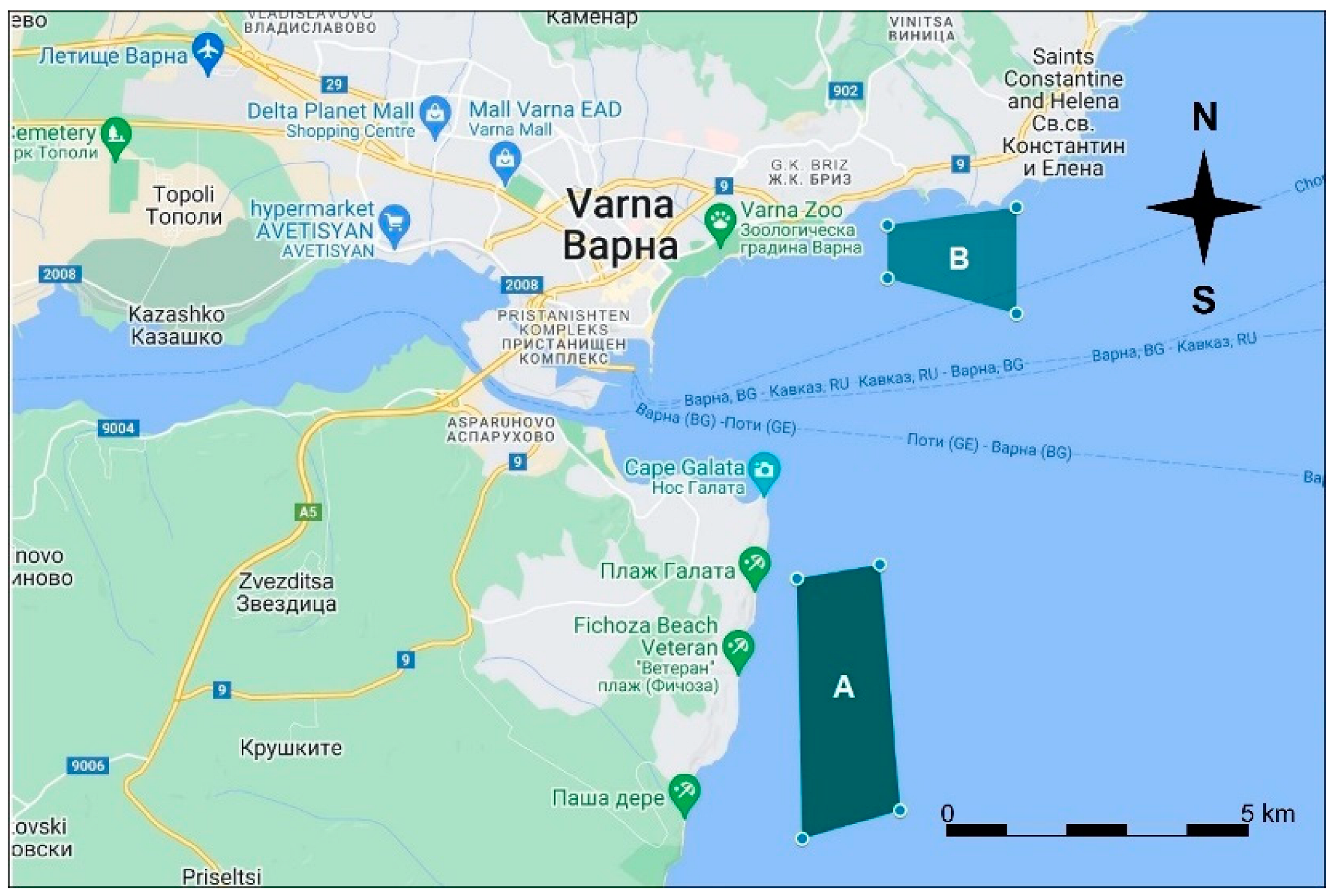
Due to ship traffic and queuing, air pollution analysis must consider weather conditions and installed ship engine power. The weather descriptors involved in the analysis are wind speed, direction, and insulation. The parameters involved in generating ship air pollution are the number of queuing ships, installed engine power and queuing time. In general, several aspects concerning air pollution are considered: the green environment, economic benefits, and shipping perspective. Different sources of information for the seaport of Varna are incorporated in the developed framework for evaluating air pollution due to shipping traffic in the coastal zone. Currently, the port of Varna does not have a monitoring system to control air pollution. The developed framework uses information from the existing internet ship traffic control system and local weather forecast control station. Employing the extreme value theory, Weibull frequency distribution and Gaussian air pollution model, the risk of generating and the spread of air pollution are estimated. The analysed seaport (B) is in the vicinity east of Varna (Figure 1).

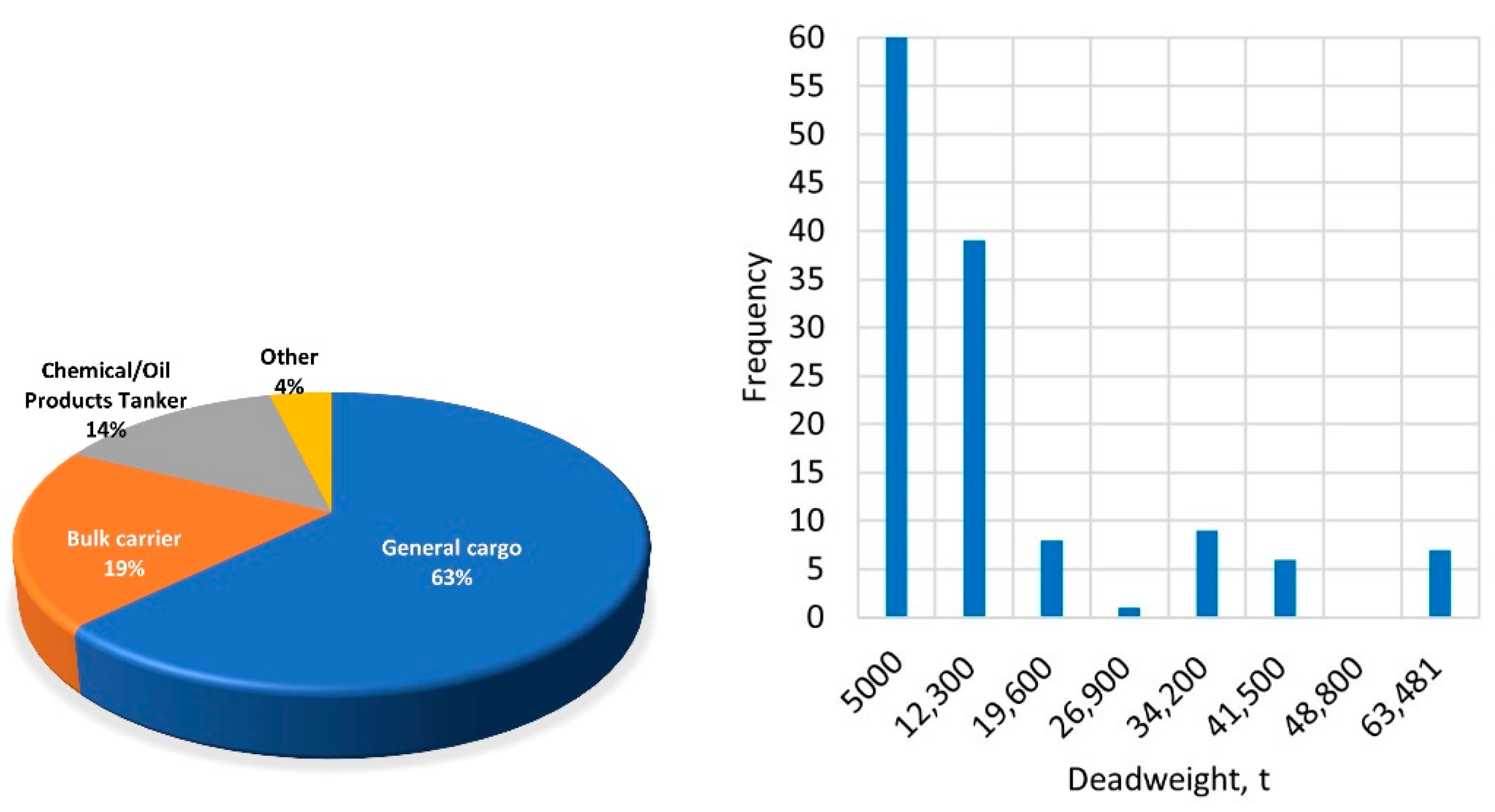
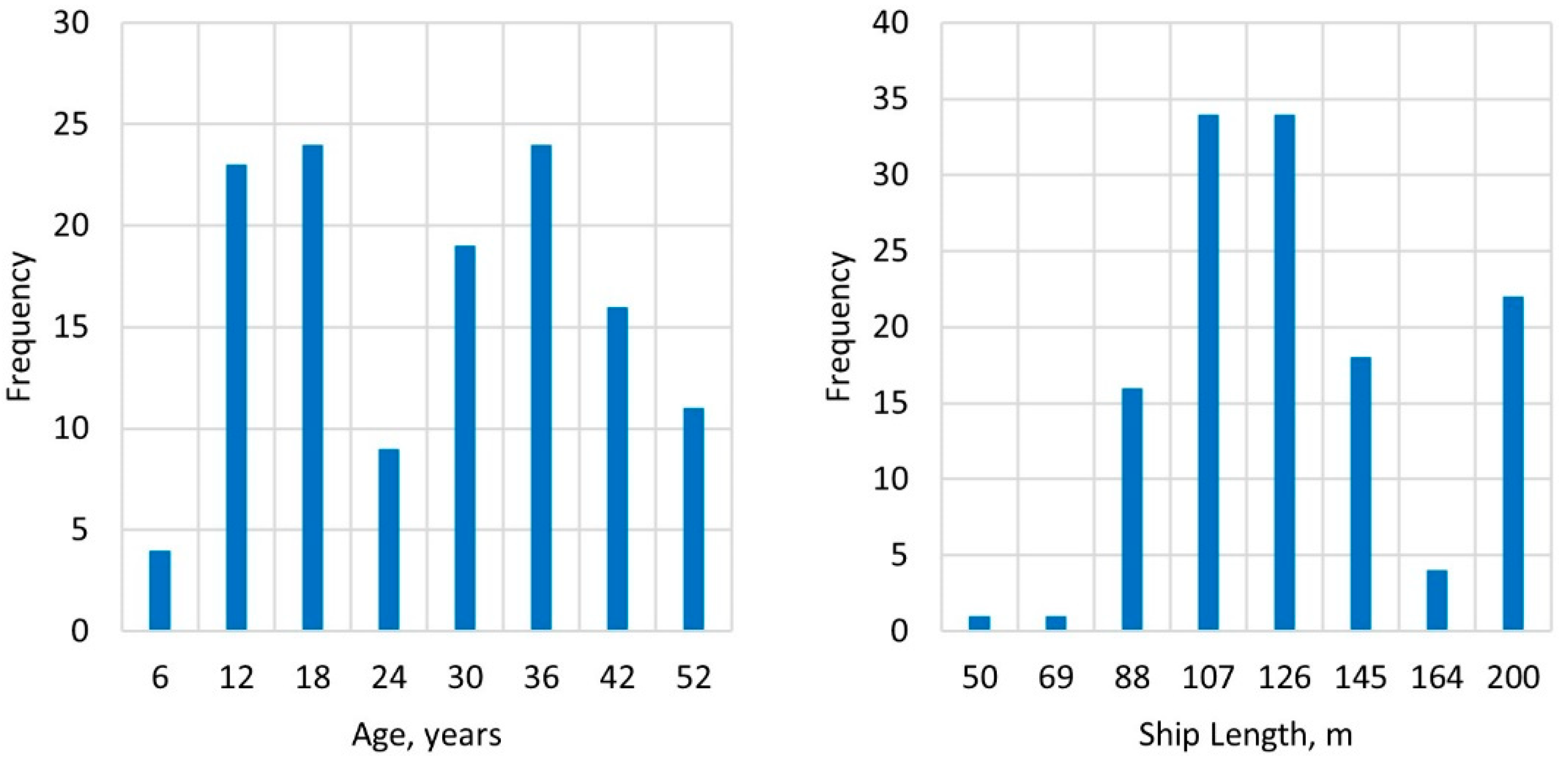
The types of the 130 ships anchored in the seaport of Varna from November 2021–April 2022 are shown in Figure 2, (left) where it can be seen that 63% of the ships are general cargo ships, followed by 19% bulk carriers, 14% chemical/oil product tankers and the rest is 4%. The DW of the anchored ships ranges from 1412 to 63,481 tonnes, shown in Figure 2, (right). The ships’ ages vary from 2 to 52, with an average of 25 years (see Figure 3, left). The minimum length is 41.33 m, and the maximum is 199.98 m, with an average of 119.62 m (see Figure 3, right).

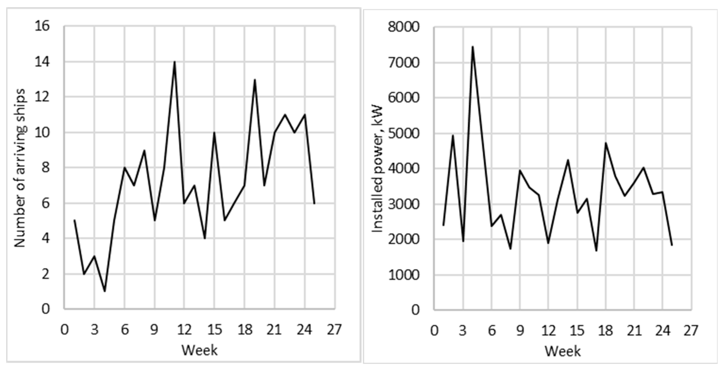
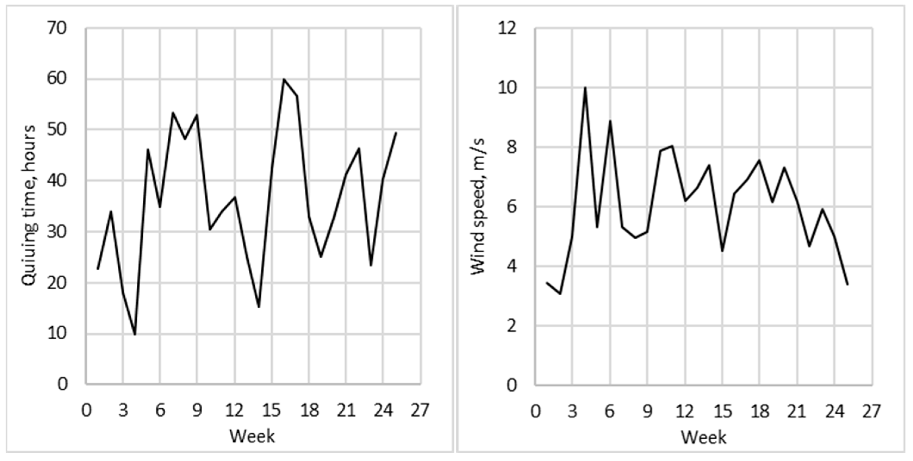
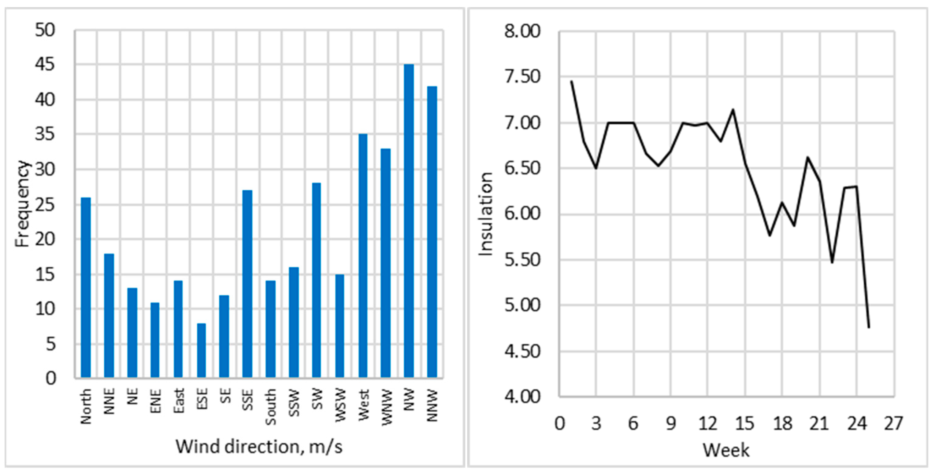
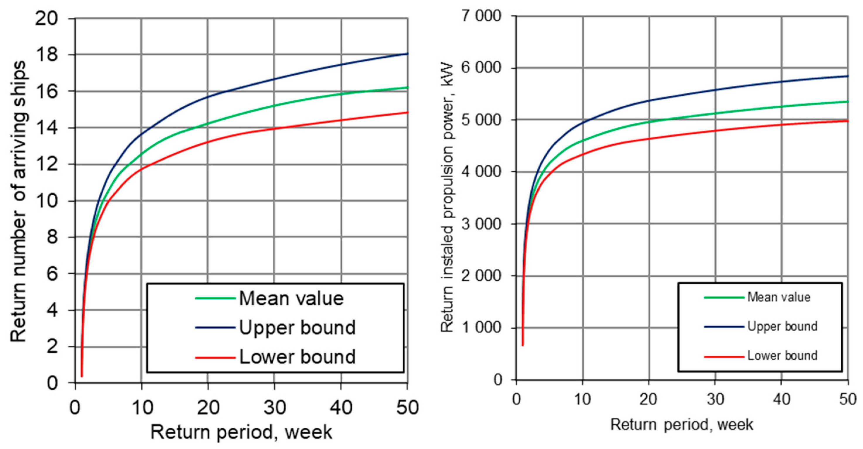
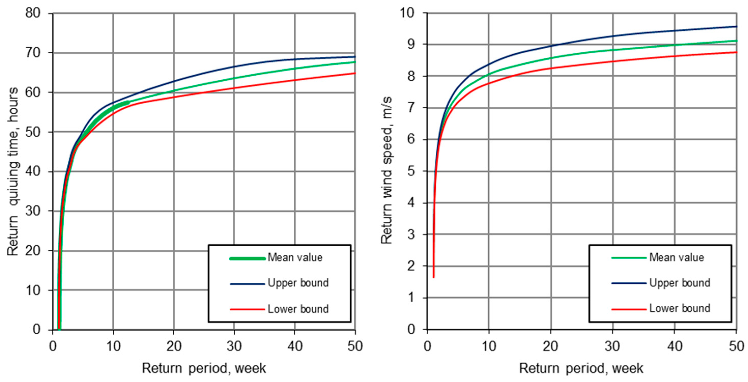
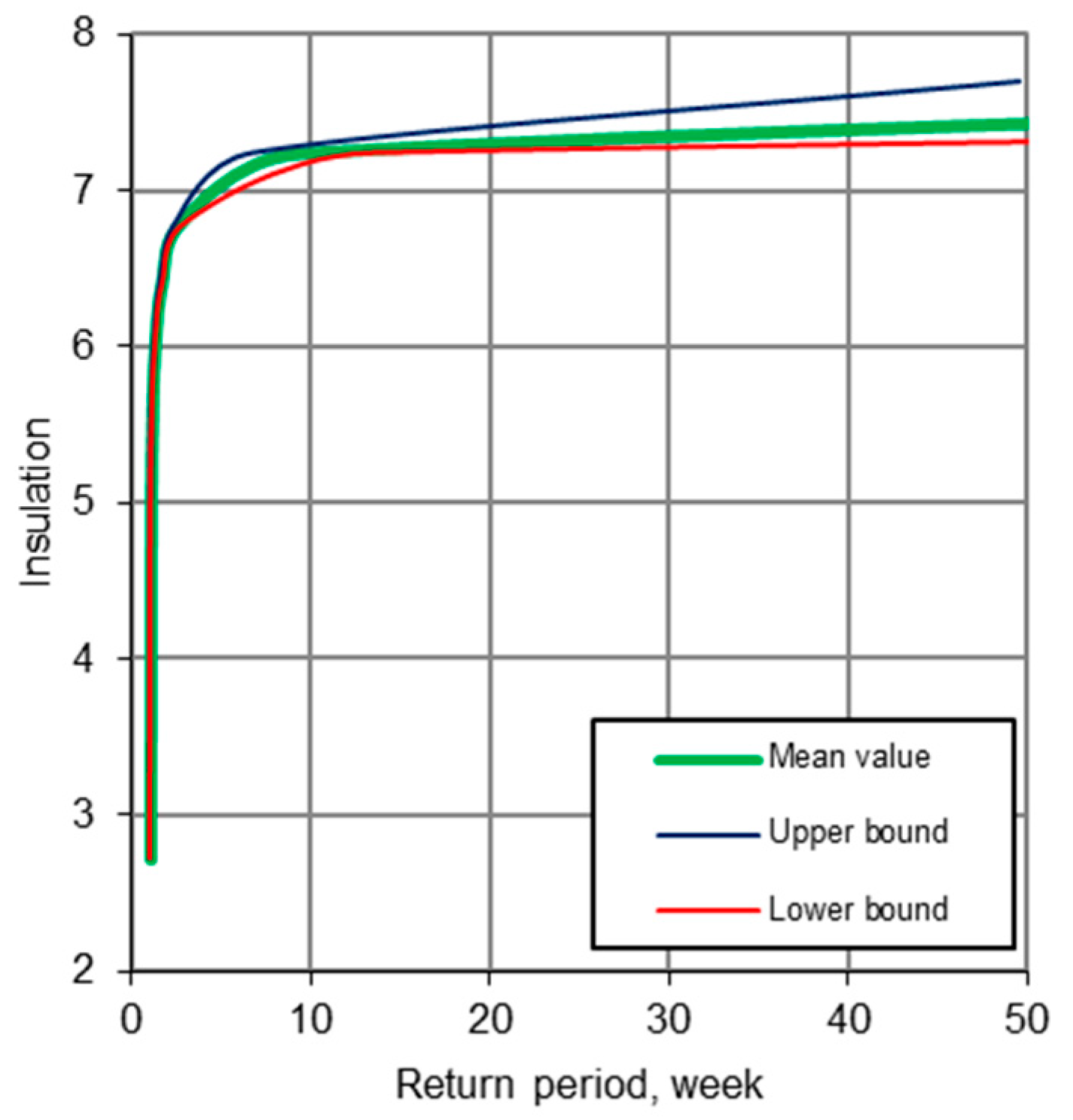
The generated pollution due to the queuing ships in the seaport may be defined as a function of the installed propulsion power, accounting for the wind and weather scenario. The ship characteristics include the ship’s installed engine power, the number of arriving ships, queuing time and the weather conditions, and wind speed, direction, and insolation. The average weekly installed engine power of the number of arriving ships, queuing time, wind speed, wind direction, and insolation for 25 weeks (November 2021–April 2022) for the winter season are given in Figure 4, Figure 5 and Figure 6.

Wind speed and direction are essential governing factors in the dispersion and transport of air pollution concentration. Wind reduces air pollution concentrations inversely proportional to wind speed downwind of air pollution sources. Analysis of wind shows that winds are generally strong in the seaport. The weekly average wind speed varies from 3 to 10 m/s (Figure 5 right). Northwest is the dominant wind direction, followed by NNW and W in the seaport area (Figure 6, left).

Atmosphere stability is related to resisting or enhancing turbulence, which significantly affects the concentration of a pollutant. In this respect, the more unstable the atmosphere is, the more pollutant dilution there is. Stability classes are used for different weather conditions, which are a function of wind speed and solar insolation during the day and cloud cover during the night. Classes A, B, and C stand for volatile, unstable, and slightly unstable conditions, respectively; D stands for a neutral condition; and E and F stand for stable and very stable conditions, respectively. Class G represents the most stable atmosphere possible and is used for the worst-case simulations. Classes of atmospheric stability depend on wind speed, as stipulated in [41].

For the region of the Varna seaport, a 25-week statistic for the winter season is collected. The average weekly atmosphere stability is given in Figure 6, right, where the alphabetic class notation from A to D is presented in a numerical notation, where A = 1, A-B = 2, B = 3, B-C = 4, C = 5, C-D = 6, D = 7, E = 8, F = 9. It can be noticed from Figure 6, right, that the predominant class of stability is D = 7.

The statistical descriptors of the Weibull distribution for the analysed data in Figure 4 to Figure 5 are shown in Figure 7, Figure 8 and Figure 9.

3. Extreme Value Analysis

The study employs extreme value analysis as a statistical treatment used to estimate the probability of an unacceptable parameter value. For example, short-term exposure can also cause serious health problems. In this regard, extreme value analysis can be seen as a fundamental statistical approach to assess the incidence of exposure peaks to which a given geographical area is subjected.

The extreme value can be characterised by three parameters, shape $\xi ,$ location $\mu$, and scale $\sigma$ [46,47,48], which describe the behaviour of the extreme value distribution as:

$$F\left(x, \mu ,\sigma ,\xi \right)=exp\left\{-{\left[1+\xi \left(\frac{x-\mu }{\sigma }\right)\right]}^{\frac{-1}{\xi }}\right\}$$

(1)

The shape factor governs the tail behaviour, and the subfamilies which are defined by a shape of 0, bigger than 0, and less than 0 correspond to the Gumbel (type I), Fletcher (type II) and Weibull (type III) distributions, respectively [48]. In the present study, the Weibull distribution function for describing extreme values of the weekly maximum of air pollution is used due to its simplicity and flexibility.

Extreme events may also be related to their return period, $P_r$, where for any given period, the probability of occurrence is defined as $Q=1/P_r$, and the risk is defined as the probability that one or more events will exceed a given threshold within a specified period. The risk, $R$, is calculated using the binomial distribution as $R=1-{\left(1-Q\right)}^n$, where $n$ is the number of periods.

The information on return periods can benefit policymakers in making decisions based on the expected maximum weekly return values. The return values of arriving ships and installed propulsion power are shown in Figure 10, queuing time and wind speed are given and Figure 11 and insolation in Figure 12. They will be used to predict the air pollution generated by the queuing ships and the probability of spreading to the cost.

4. Gas Emissions and Air Pollution

The gas emissions are defined as a function of the installed propulsion power, the number of encountered ships in the seaport and queuing time. For calculating the gas emissions, factors defining propulsion and auxiliary engine factors are estimated, defining the time of ship operational activity in queuing and the voyage duration. The factors used for calculating the gas pollutants are $L{F}_{PE,i}$, which is the propulsion engine load factor, $L{F}_{AE,i}$ is the load factor of the auxiliary engine, and $T_i$ is the time of the ship operation during the queuing at the seaport. The load and time factors for propulsion and auxiliary engines are assumed as $L{F}_{PE, queuing}=20\%$, $L{F}_{AE, queuing}=50\%$. A more profound analysis of engine load for the different operational activities can be seen in [49,50] among others.

The ships analysed here are assumed to be medium-speed diesel, MSD and use marine diesel oil, MDO, and the emission factors [49] used in the analysis are $E{F}_{PE, {NO}_x }=10.6 \mathrm{g}/\mathrm{kWh},$ $E{F}_{AE, {NO}_x }=13.9 \mathrm{g}/\mathrm{kWh}$.

The gas emissions, $Q_{queuing}$ is estimated by multiplying the time spent with the total installed propulsion, $P_{PE}$ and auxiliary, $P_{AE}$ engine power, engine loading and the operational and emission factors for propulsion, $E{F}_{PE,i}$ and auxiliary, $E{F}_{AE,i}$ engines. The emissions for the $n$ ships queuing in the seaport are calculated as follows:

$$\begin{gathered} Q_{queuing}={{\displaystyle \sum }}_{i=1}^n\left[\left(P_{PE,i}L{F}_{PE,queuing,i}E{F}_{PE,{NO}_x,i}\right)+ \\ \left(P_{AE}L{F}_{AE, queuing,i}E{F}_{AE,{NO}_x,i}\right)\right]T_i \end{gathered}$$

(2)

The Gaussian dispersion model [40,41,42] is used for estimating the air pollution concentration for a specific period:

$$\begin{gathered} C_{i,j,k,l,m}\left(x,y,z\right)= \\ \frac{Q_{queiuing,i,j,k}}{\pi {\sigma }_{y, i,j,k,l,m}{\sigma }_{z,i,j,k,l,m}{u}_i}exp\left(-\frac{1}{2}{\left(\frac{y}{{\sigma }_{y,i,j,k,l,m}}\right)}^2\right)exp\left(-\frac{1}{2}{\left(\frac{H}{{\sigma }_{z,i,j,k,l,m}}\right)}^2\right) \end{gathered}$$

(3)

where $Q_{qeuiuing,i,j,k}$ is the emission rate, where $i,j,k$ are indexes related to the number of queuing ships, installed engine power and queuing time, respectively, ${\sigma }_{y, i,j,k,l}$, ${\sigma }_{z, i,j,k,l}$ are the dispersion coefficients as a function of $x$ and $y$ representing the longitudinal and transverse distances from the seaport, representing the source of pollution, $u_l$ is the wind speed, and $H$ is the effective stack height. The air pollution concentration in each point $x, y$ and z is proportional to the $Q_{qeuiuing,i,j,k}$ and inversely proportional to $u_l$. The dispersion coefficients ${\sigma }_{y,i,j,k,l,m}$, ${\sigma }_{z,i,j,k,l,m}$ are a function of the receptor position, and $m$ represents the weather stability conditions.

The Gaussian dispersion model is developed using the general transport-diffusion assuming the stationary process with no change in time, homogeneous and flat spatial domain, and wind speed [40,41,42].

The emitted pollution from the queuing ship is integrated into a point source of pollution, and the dispersion of the air of pollutants is modelled for $z$ = 0 surface level. The queuing ships will accumulate concentrations in the receptors along $x,y,z$, where $z$ =0.

The Monte Carlo approach [51] is employed to model the uncertainty propagation in the air pollution estimates generated by the stochastic input variables related to the number of queuing ships, installed engine power, queuing time, wind speed and insolation. The air pollution concentration $C_{i,j,k,l,m}\left(x,y,z\right)$ is estimated for $n$ stationary conditions.

$N{O}_x$ emissions are the highest compared to other pollutants from the diesel exhaust of ships. The variations in $N{O}_x$ emissions are considered a significant trend of emission patterns of the gases generated by ship engines and emitted into the atmosphere, which are directly related to fuel consumption. The pattern of other air pollutants is very similar to that of $N{O}_x$ emissions. There has been a steady increase in annual $N{O}_x$ emissions in the last ten years. The maximum allowable concentrations considered here is $C_{MAC,N{O}_x}$ = 25 μg/m³; more information can be seen in [52].

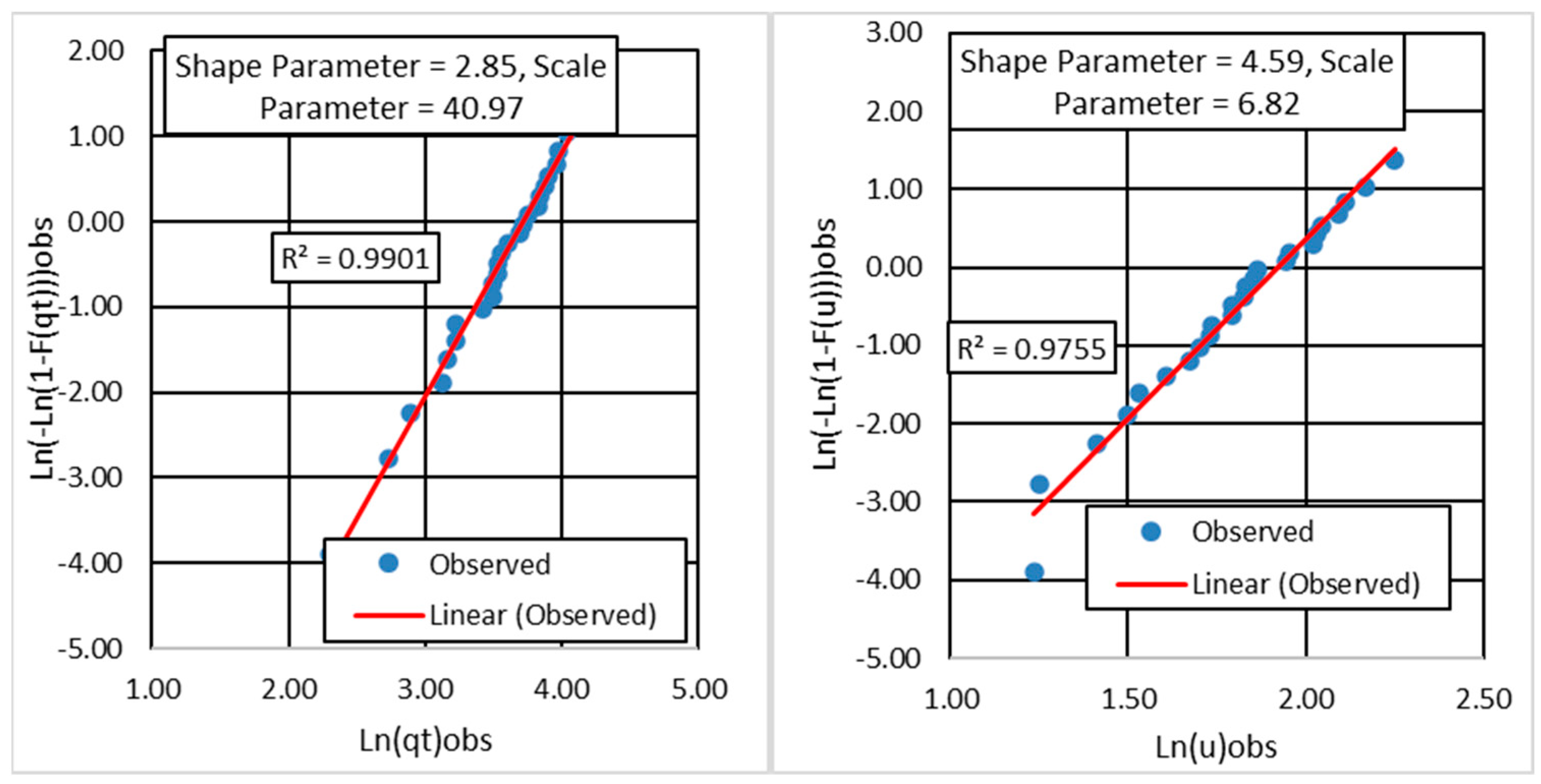
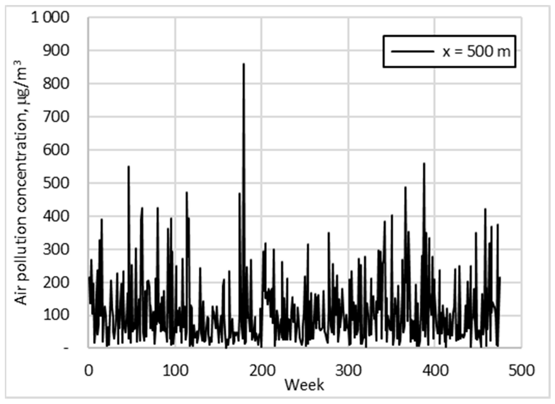
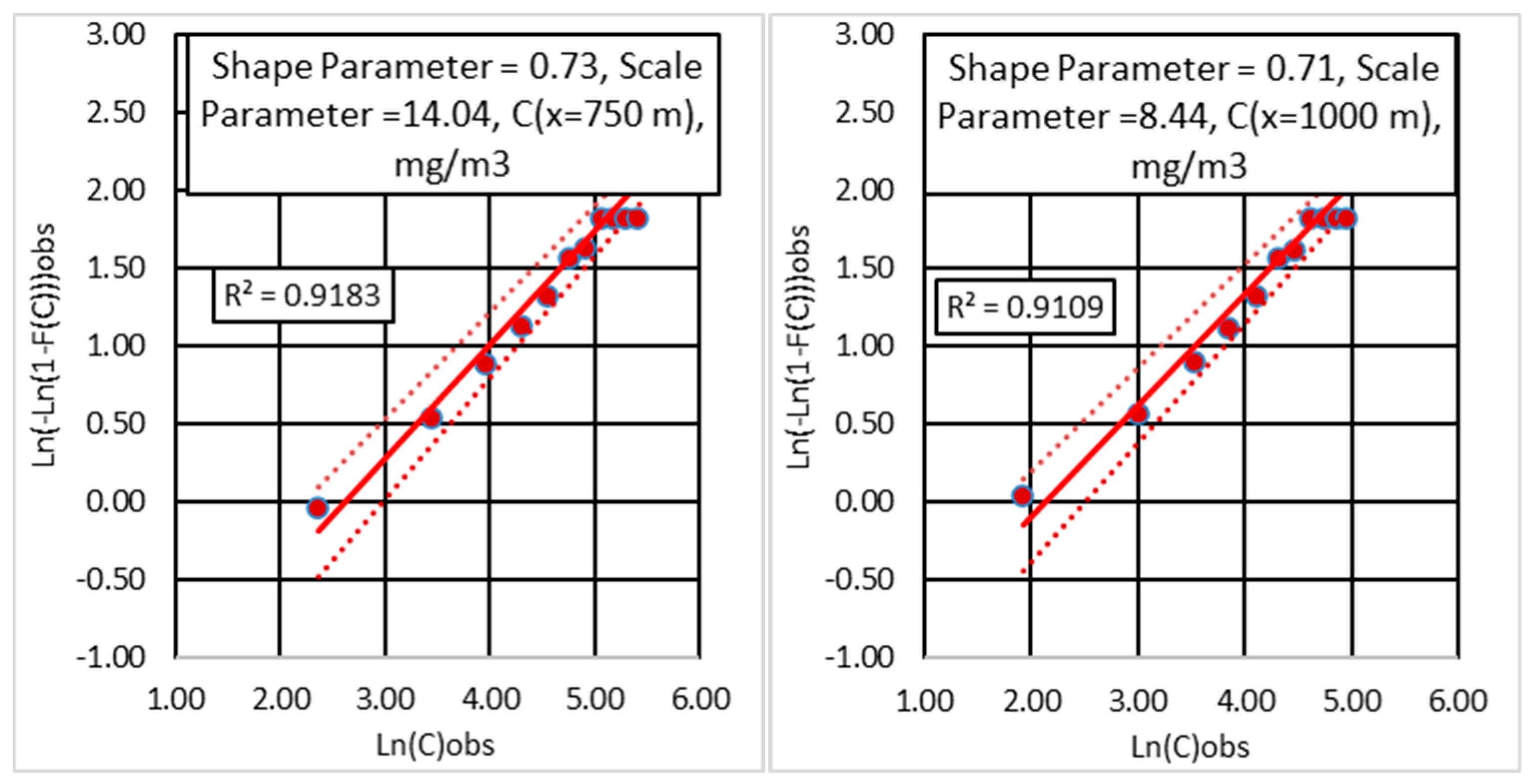
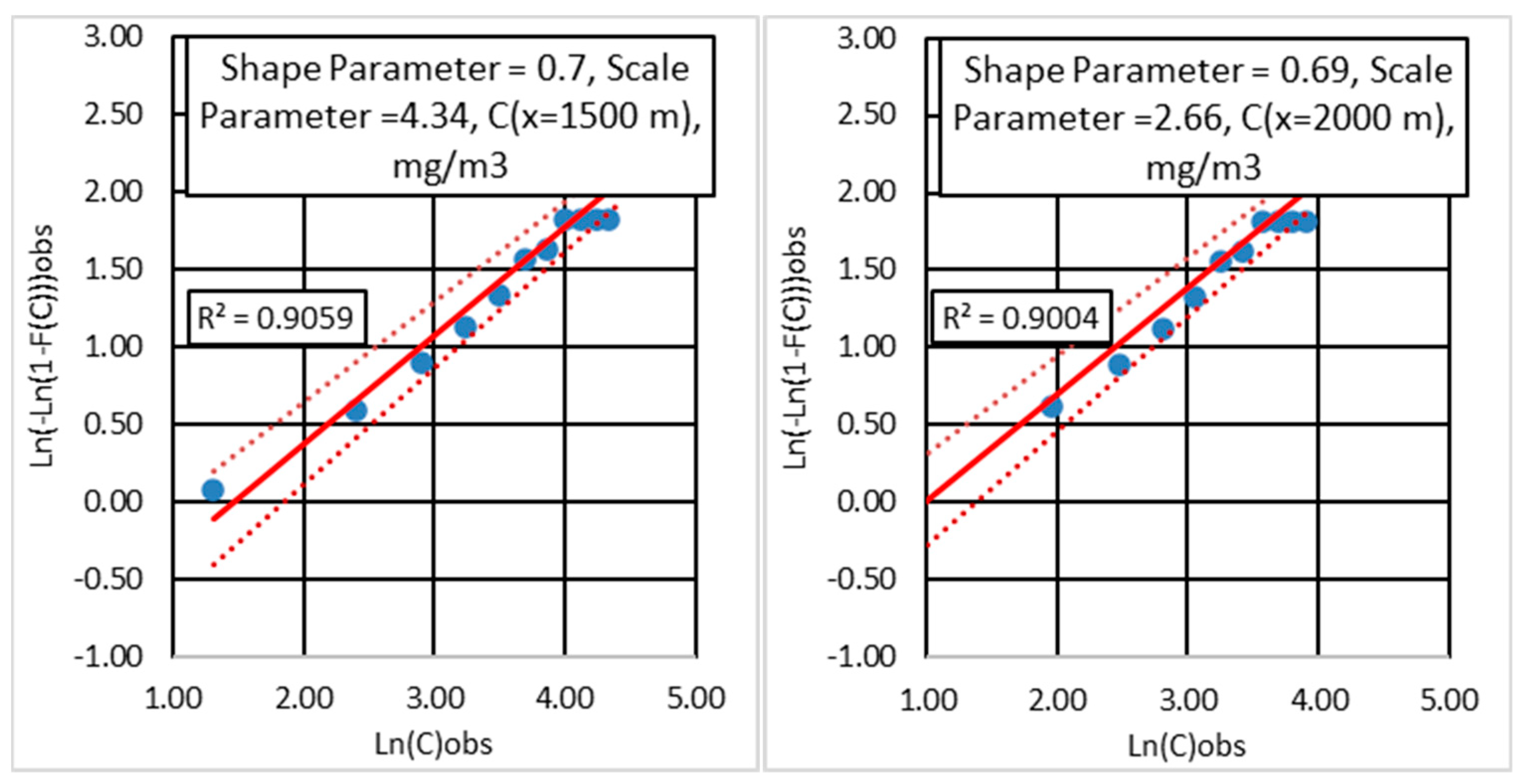
The Monte Carlo air pollution concentration, $C\left(x,0,0\right)$ generation for x = 500 m is shown in Figure 13, and Weibull distribution descriptors along the x-directions in the range from 500 m to 2500 m are shown in Figure 14, Figure 15 and Figure 16.

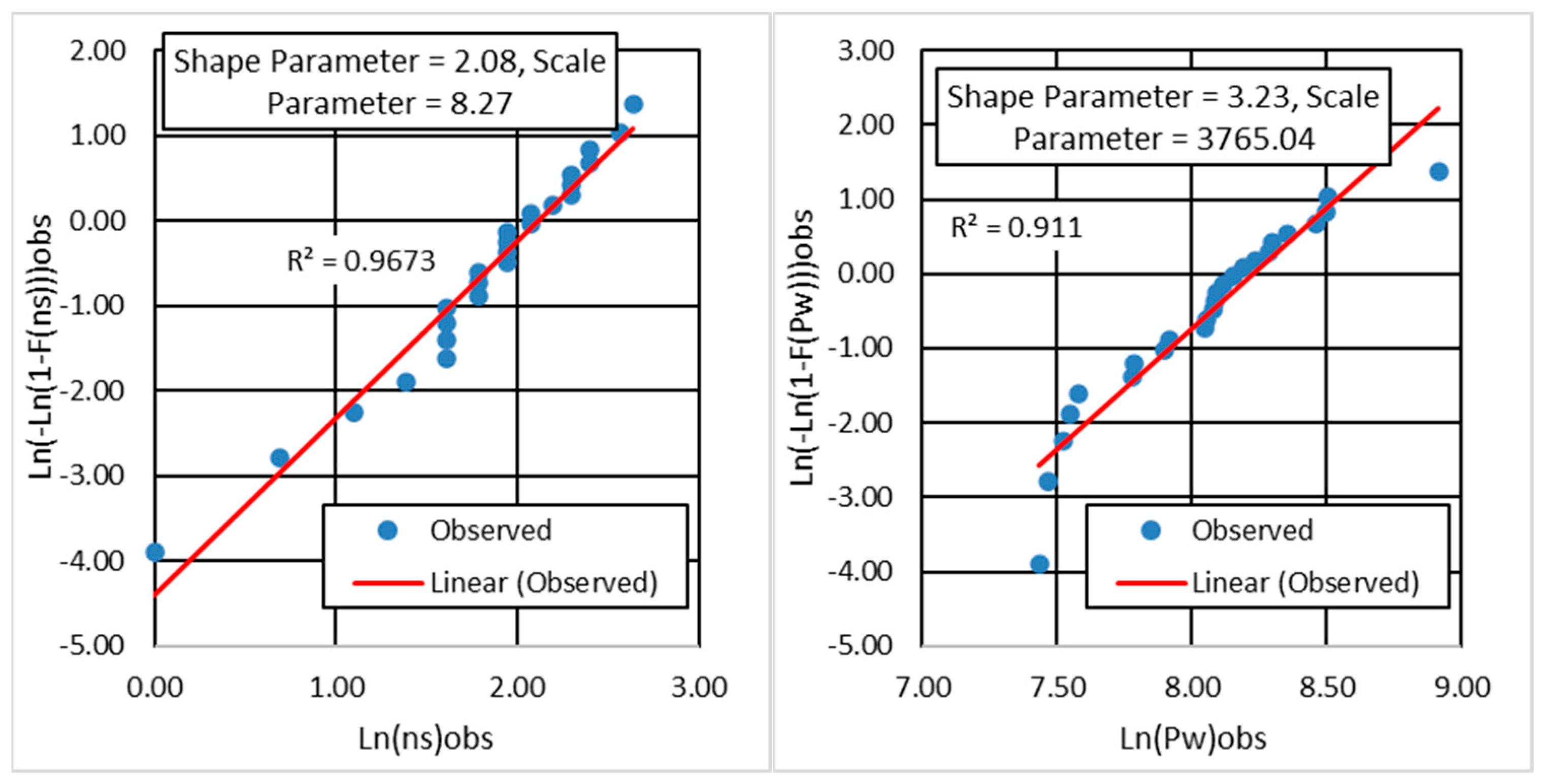
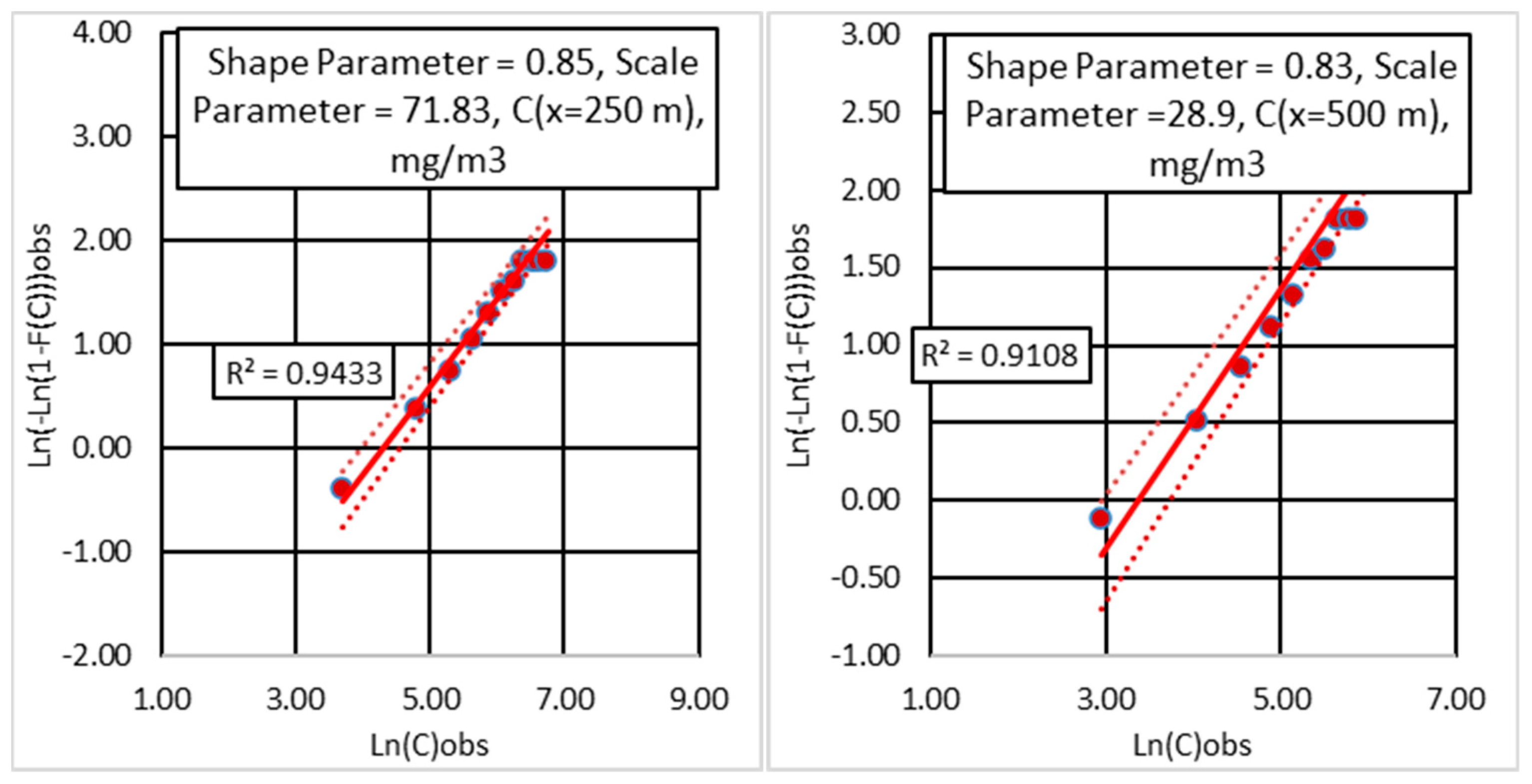
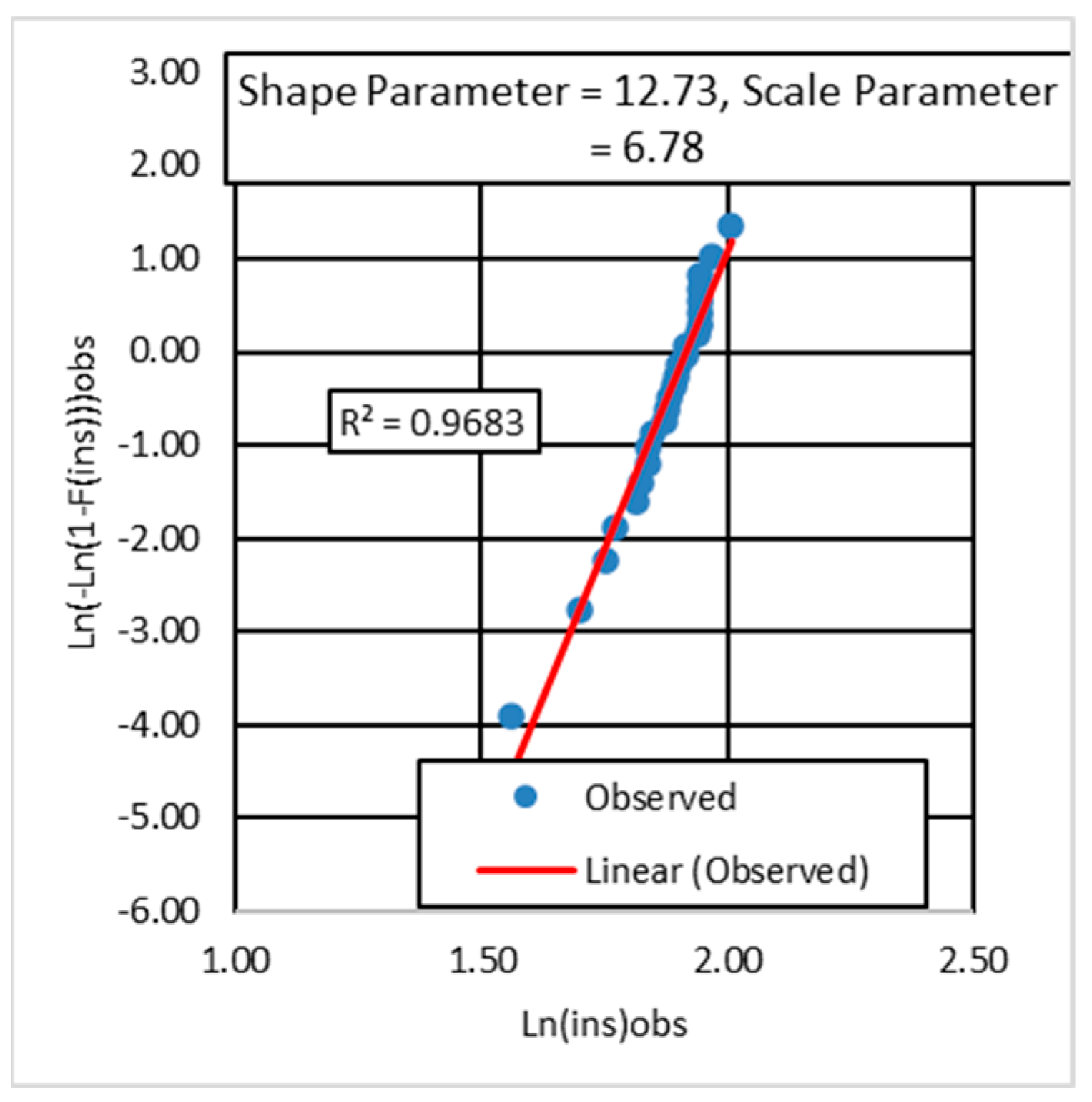
The generated data for the air pollution concentration for x = 500 m is shown in Figure 11, and Weibull distribution descriptors along the x-directions in the range from 250 m to 2000 m are shown in Figure 12 to Figure 14, where it can be seen that the shape factor varies between $0.69 \mathrm{and}$0.85. The Weibull fitting is shown by a double log scale where R² in all cases is between 0.9 for x = 2000 m and 0.94 for x = 250 m distance from the source of pollution. The shape factor tends to be smaller for the geographical locations away from the source of pollution. The data following the Weibull distribution are independent and identically distributed, which can be used to obtain satisfactory statistical conclusions in applying the extreme value theory.

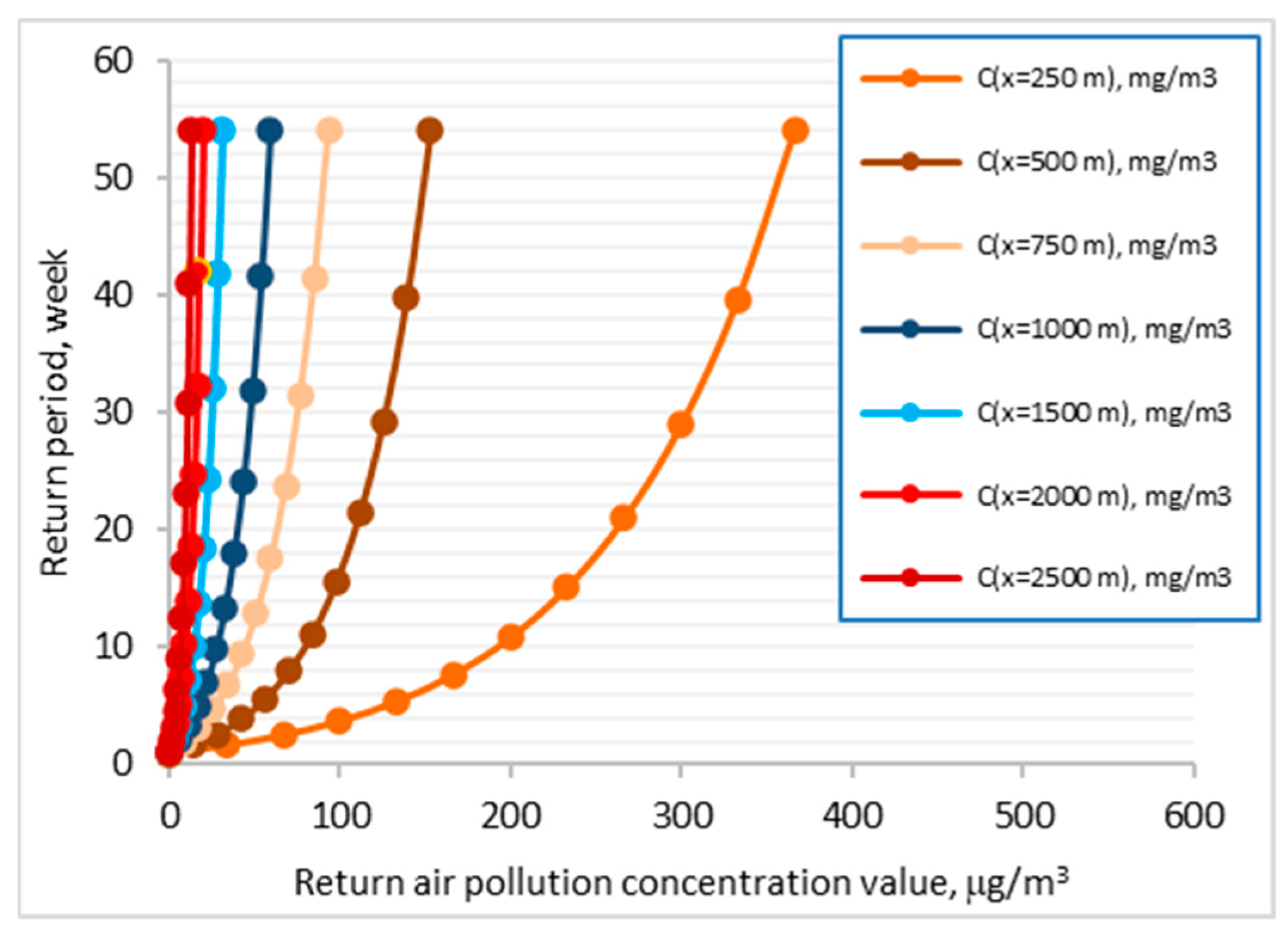
The return period is the estimated time of the occurrence of peak levels above thresholds to find the conditions that define the highest probability of extreme values. Although distribution shape parameters may help identify the places with a greater chance of extreme concentrations, the probability is also influenced by other distribution parameters. The present study only calculated the probability and return period for the extreme value analysis, employing the Weibull distribution.

The analysis of the air pollution frequency relates the magnitude of a given air pollution event with the frequency or probability of that event’s exceedance. In performing a frequency analysis of the air pollution peak, several assumptions are imposed, including data independence, data sufficiency, weather description, ship traffic, and the reliability of air pollution estimates. The air pollution estimates provide random, independent event data. Otherwise, the resultant distribution of air pollution frequencies may be significantly biased, leading to inappropriate estimations. Performing a peak air pollution frequency analysis, the data points used are independent and unrelated. The analysed data contain enough periods of consecutive air pollution peak data to minimise bias. However, longer records are generally recommended to estimate more considerable return periods and/or if there is a potential bias in the data set. Using data that fully captures the peak for peak flow analysis is also essential.

Figure 17 shows the plots obtained from applying the extreme value approach for the seaport of Varna. The plots are for $N{O}_x$ air pollution as a function of the distance of the pollution from the seaport.

The results from extreme value indicate that the return period can be from 3 to 4 weeks for different distances from the source of pollution of $25 \mathsf{\mu }\mathrm{g}/{\mathrm{m}}^3$. However, 250 m shows the highest number of exceedances and 2500 m the smallest one.

5. Air Pollution Dispersion

The analysed air pollution concentrations may be employed to resolve different environmental problems, including defining the maximum air pollution emission rate that needs to be an acceptable limit conditional on the probability of exceedance in a specific period, and additionally, what will be the abatement cost of air pollutant originating from the anchored ships in the seaport to guarantee a clean environment in the populated coastal zones [43]. It is also essential to identify the significance of pollution emissions in the coastal populated zones that will permit determining the tolerable pollution concentration at the seaport location, leading to specific abatement rates for the anchored ships. Consequently, all these are to identify the best position of a seaport where the queuing ships may anchor without perturbing the population’s daily life in the coastal zone.

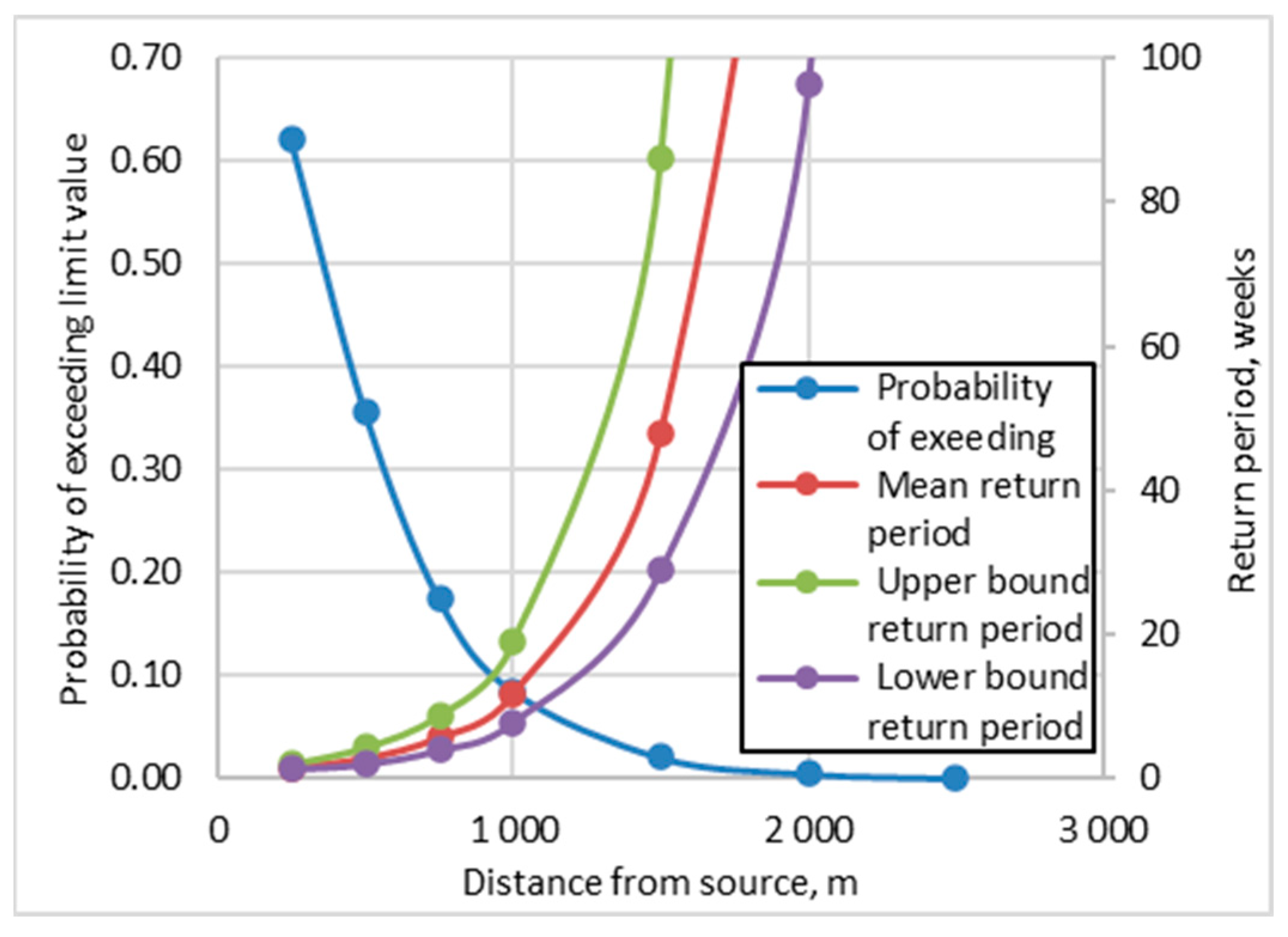
The analysed receptors, located in the coastal zone, are part of one ecosystem. The probability that the air pollution $N{O}_x$ concentration would exceed the limit value of $25 \mathsf{\mu }\mathrm{g}/{\mathrm{m}}^3$ and its corresponding return period is given in Figure 18 for different distances from the anchored ships waiting to enter the port. The probability that the largest $N{O}_x$ concentration at x = 250 m would exceed the limit value is 0.62, which corresponds to a return period of 1.61 weeks. The largest $N{O}_x$ concentrations for the one year, 54 weeks, is about $366 \mathsf{\mu }\mathrm{g}/{\mathrm{m}}^3$.

Controlling the air pollution level estimates the risk of the spread of air pollution, and its consequences are estimated as follows:

$$R(x,y,\theta , T_r)=P_r\left(C(x,y | T_r)>C_{MAC,N{O}_{\mathrm{x}}}\right)P_r\left(\theta \right)C_n\left(x,y\right)$$

(4)

where $R(x,y,\theta , T_r$) is the excess lifetime risk in a monetary term for a return period $T_r$, C$(x,y | T_r$) is the air pollution concentration, $P_r\left(\theta \right)$ is the probability of wind direction $\theta$, $C_n\left(x,y\right)$ is the consequences of cleaning air pollution and eco damage in monetary terms.

The consequence measures in monetary terms to keep the environment safe is defined as:

$$C_n\left(x,y\right)=G_{cl}+G_{eco}+G_{port}$$

(5)

where $G_{cl}$ is the cost needed for cleaning (abating) the air pollutants at the seaport, $G_{eco}$ is the eco damage due to the air pollution gases generated by the ship’s engines. The excess air pollution concentration is removed using different air pollution systems, including scrubbers, to reduce the air pollution concentration to an acceptable level, and $G_{port}$ is the cost associated with the services that anchored ships need to be provided by the port, which is directly proportional to the distance between the port and the seaport.

The pollution discharge needed to be removed (abated) is estimated as $C_a$ and the cost associated with that is defined as:

$$G_{cl}={\displaystyle \sum }_k{C}_a{G}_{air,k}$$

(6)

where $G_{air,k}$·is the cost associated with the air pollutant cleaned by $k$^th ship at the seaport that needs to be cleaned [53].

To mitigate the pollution level from different ships (sources) anchored at the seaport, an optimisation procedure is employed, where the gas emission, represented as a source of pollution, is reduced to meet the maximum allowable concentration standards by minimising the air pollution cost expenses, cleaning only the excessive emission.

The factor of reducing the air pollution generated by the k^th ship anchored at the seaport is defined as $w$ = ($w_1$,…, $w_n$) ∈ [0, 1] and the total cost of cleaning is assumed to be a linear function of $w_k$ defined as:

$$G_{cl}={\displaystyle \sum }_k{C}_a{C}_k{w}_k$$

(7)

Recently an intensive discussion related to the cost of air pollution can be seen in many studies [53], where for scrubber and catalytic conversion, the cost assumed for removing $N{O}_x \mathrm{is} \mathrm{about} 0.55 \mathrm{EUR}/\mathrm{kg}$ [45].

The damage to the ecosystem estimated in a monetary unit, $G_{eco}\left(\mathrm{x},\mathrm{y}\right)$, is defined as:

$$G_{eco}\left(\mathrm{x},\mathrm{y}\right)=Q_a\left(\mathrm{x},\mathrm{y}\right)G_{eco}$$

(8)

where $G_{eco}$ denotes the damage cost of the pollutant $N{O}_x$, EUR per $\mathsf{\mu }\mathrm{g}/{\mathrm{m}}^3$ and $Q_a\left(\mathrm{x},\mathrm{y}\right)$ is the emission rate after the abatement. The average health damage costs is defined by the national agencies for maritime emissions related to the health effect, crop loss, biodiversity loss, material damage etc.; the average damage cost for $N{O}_x$ is 7.8 EUR/kg [44,54]

The seaport area is established by accounting for environmental and economic conditions defining the anchoring area as a polygon. Depending on the services needed and the distance between the port and the seaport, the cost is defined here as $G_{port}$ and may vary from port to port.

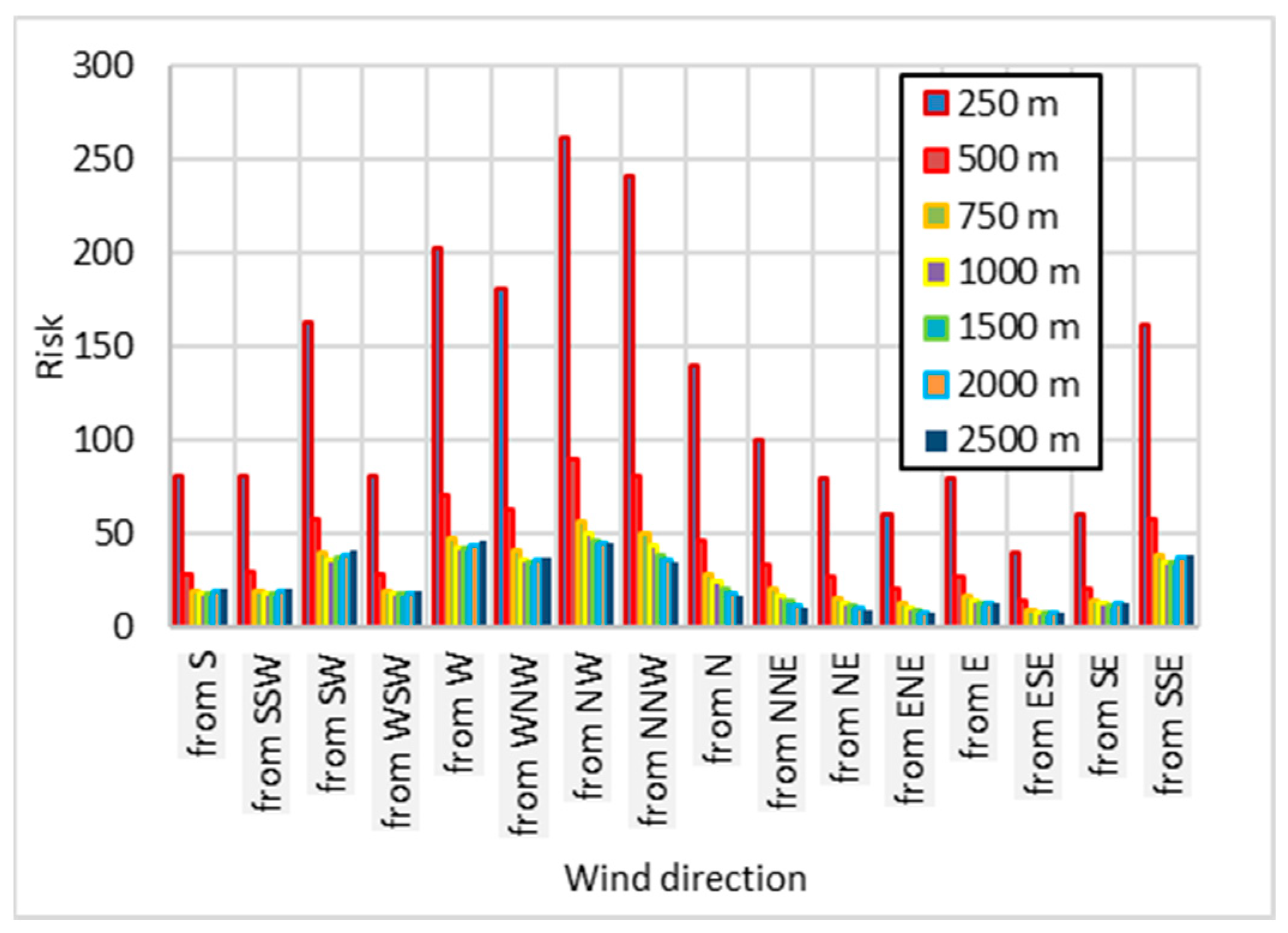
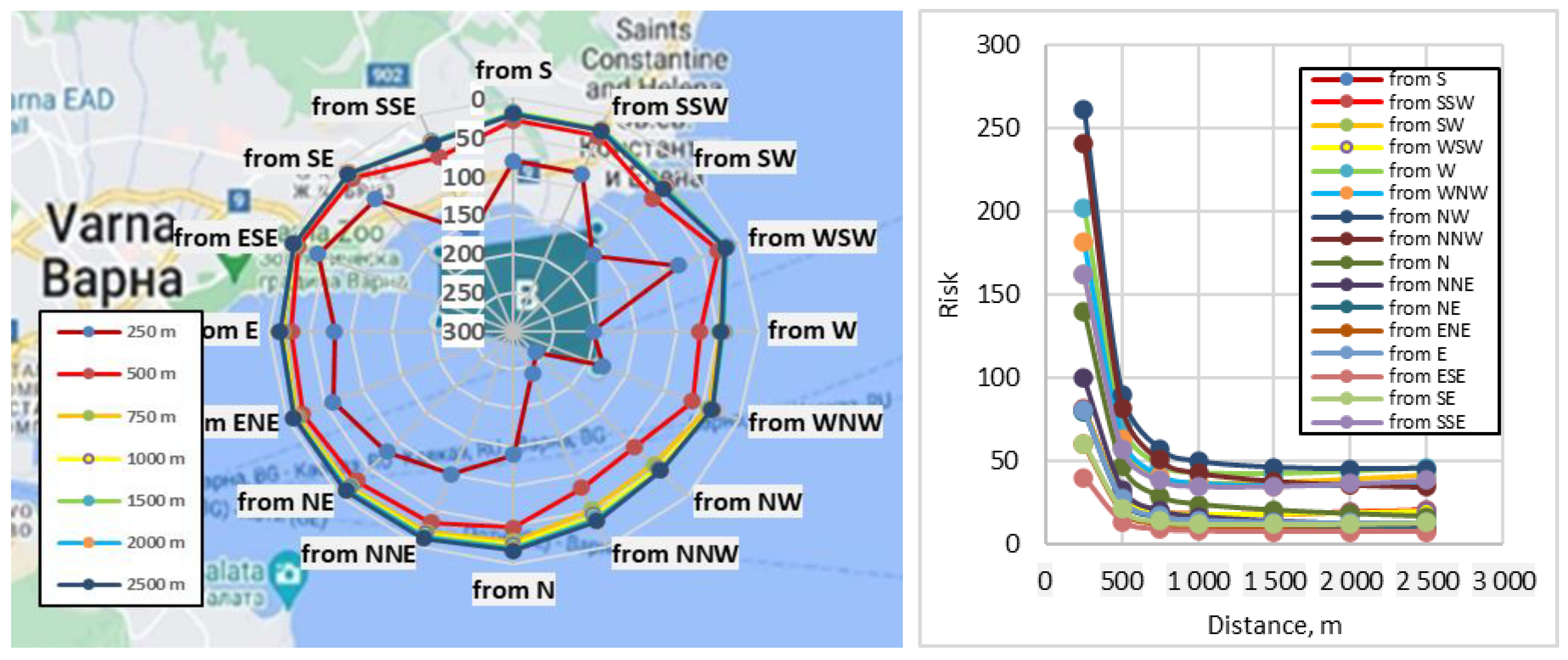
Figure 19 and Figure 20 show that the most significant risk, as defined by Equation (7), of generating and spreading air pollution comes from the NW, followed by NNW and W. However, the air pollution dispersion is only critical because the populated coastal zone is oriented to E, NE. In this respect, the most critical air pollution the queuing ships generate is E to S.

Figure 20 (left) shows how the risk of air pollution spread is projected to the seaport map and coastal zone as a function of distance, conditional to wind direction, in one year return period. Figure 20 (right) presents how the risk is spread as a function of the distance from the source of pollution (winter Seaport).

The approach developed here can solve different problems, including the maximum emission rate, minimum abatement cost needed, the significance of pollution emissions, and tolerable air pollution concentration, to find the most suitable position of the seaport and acceptable intensity of ship traffic etc.

Analysing air pollution, including NO_x emission, by employing a numeric-empirical model will not be as good as if real measurements are performed. In the present study, for the analysed seaport, such measurements are only planned for the future. To analyse the current pollution degree, a numeric-empirical model is developed based on existing practice, which was initially calibrated for different environmental conditions and port activity and supplied by the data originating from the seaport of Varna. The present study has limitations in the accuracy of the air pollution prediction. However, at present, it seems to be a suitable model that can be used to estimate air pollution, the probability of exceedance of the acceptable level of pollution, the associated risk for the population in the vicinity of the source (seaport) of pollution and its consequences. More work is needed, and the first step to create a system for collecting, analysing, and providing solutions for mitigating air pollution due to shipping urgently needs to be developed

6. Conclusions

The important result of this study is the estimation of extreme value and the return period of air pollution due to oxides of nitrogen generated by ships while queuing in the winter seaport. Original data has been collected for arriving ships, installed propulsion system, queuing time, speed and direction of the wind and weather stability for the winter season of the seaport of Varna. Analysing the risk, the time return period can be used to estimate the maximum air pollution, probability of exceedance and its consequences. Knowing the pattern of extreme air pollution can keep the environment clean, reduce ship traffic, and force the use of more environmentally friendly fuel and green ships. It is also essential to draw attention to the values identified around the seaport, which are higher than those recommended by international standards and can endanger the population’s health. The developed stochastic model can provide beneficial information in estimating air pollution. The model depends on the extent of data analysed, where more comprehensive data better represents the overall air quality characteristics. In this respect, a system of collecting data from accurate measurements needs to be established. All areas with excessive air pollution need to be covered by the existing standards of the Emission Control Areas. A step further will be to apply the developed approach to extend the data used for predicting the air pollution concentration, and to integrate it into an emission control area where all seaports used for anchoring ships will be included, to control and mitigate the ship traffic as a function of the air pollution quality level and its consequences in monetary terms.