Optimal Configuration of Gas Solid Separation Equipment Using Mixed Integer Nonlinear Programming

Abstract

The separation of solid particles from gas-solid process streams is an important unit operation in many chemical processes. Out of the many different types of separation equipment that are used for gas-solid separation, cyclone separators are widely used for their operational flexibility, efficiency and capital cost. This study focused on the design of an optimal configuration for several cyclones used in a fertilizer plant. The granulation step in the fertilizer plant leads to using different size cyclones and a different number of cyclones in series or parallel or a mix of both arrangements. A Mixed Integer Nonlinear Programming (MINLP) model is formulated to find the best cyclone arrangement with the optimal number of cyclones and dimensions from several combinations of 1D3D and 2D2D cyclones arranged in parallel-series for a high volume and heavy loading of solid particles. The objective function was to minimize the total cost, including the operating cost and the capital cost. The results indicated that a maximum of 90% efficiency is achieved with a parallel-series arrangement of 1D3D and 2D2D cyclones to be an optimal configuration for the maximum reduction in pollution level.

1. Introduction

Cyclone separators are an important class of separation equipment in chemical processes. In the literature, several studies, such as application of computational fluid dynamics (CFD) to analyze the gas–solid flow behavior of cyclones [1], performance evaluation of a wellhead multistage bundle gas–liquid separator [2], numerical study of the gas–solid two-phase flow in the tangential inlet cyclone separator [3], gas–solid simulations of a small cyclone separator [4], numerical assessment of the performance of pre-existing cyclone separators [5], and numerical characterization of the performance of new cyclone separators [6], have been reported on different types of cyclone separators depending on the type of feed utilized. Cyclone separators are primarily used to separate particles of a specific size, such as granular applications or in the removal of pollutant particles. The driving force for the gas-solid separation consists of the centrifugal force caused by the stream passing through the cyclone. Due to this centrifugal force, heavier particles move towards the wall of the cyclone while the lighter particles concentrate towards the center and then move upwards through an inner cylindrical section. Compared to other gas-solid separation technology such as membranes or filters, cyclones are more advantageous with respect to efficiency, operational flexibility and also capital cost. Efficiency and pressure drop are two important parameters used to quantify the performance and design of a cyclone when used stand-alone or in series/parallel configuration. In general, a higher efficiency is achieved at the cost of higher pressure drop which in turn increases the operating costs. An optimal design of the cyclone or configuration of cyclones would yield higher efficiency with lower pressure drop. To achieve this, more than one cyclone is used in series and parallel configuration where the number and size of the different cyclones used can be obtained by performing optimization studies. This requires an accurate description of the behavior of the cyclone which can be achieved from experiments and/or mathematical modeling. Many studies have been conducted and reported based on experimental, theoretical, and computational research on cyclones. The majority of these studies have focused on the development of single cyclones. By using cyclones in series, a higher efficiency can be achieved at the cost of higher pressure drop, but the literature related to this configuration is very scarce [7]. Additionally, few research groups have conducted studies (e.g., implementation of mathematical programming models for optimizing the configuration of series and parallel cyclone arrangement in a fertilizer plant [8], optimization of gas cyclones operating in parallel mode [9], iterative computation approach for optimizing the number and size of parallel cyclones [10], nondominated sorting genetic algorithm (NSGA)-based multiobjective optimization of a set of identical reverse-flow cyclone separators in parallel arrangement [11], and application of geometric programming for the optimal design of cyclone separators [12]) for parallel arrangement of cyclones. Several advances in the structural optimization and also modern optimization tools have led to obtaining optimal solutions for very tedious cyclone optimization problems [13,14]. General Algebraic Modeling System (GAMS) is robust software for solving complex optimization problems which is used for the research described in this article [15]. Cyclones used in a paper mill industry [11,16] are considered for the modeling and optimal configuration. 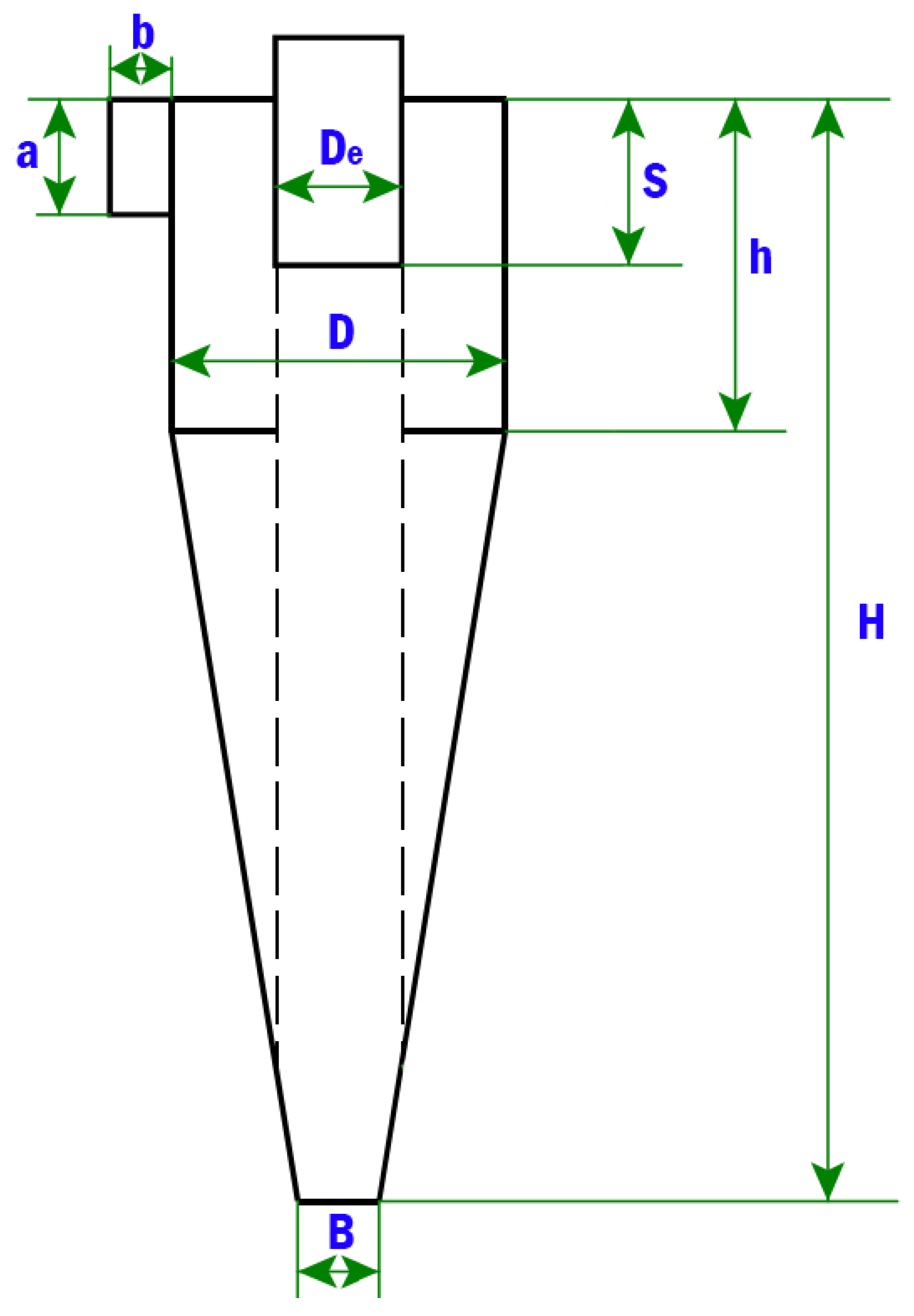The geometric parameters used to describe a cyclone are shown in Figure 1.

In Figure 1, a is the inlet height, b is the inlet width, B is the dust outlet diameter, D is the diameter of the cyclone, D_e is the gas outlet or vortex finder diameter, S is the gas outlet length, h is the cylindrical height of the cyclone and H is the overall height of the cyclone. Cyclones are also designed by using nDmD, where n and m are numbers used as multiples of the diameter to obtain the cylindrical height (h) and the conical height (H-h). For example, a cyclone represented by 1D3D means the cylindrical height is equal to the diameter while the conical height is equal to three times the diameter. By knowing these three parameters, the values of other unknown parameters (such as B, S, D_e, etc.) of the cyclone are fixed. In this article, 1D3D and 2D2D cyclones are used for optimization. Wang et al. [17,18] reported that 1D3D and 2D2D cyclones are more efficient in capturing particle diameters less than 100 nm compared to other cyclone designs. There are other experimental studies performed using these cyclones to evaluate their performance when used in series. An existing 2D2D cyclone was connected to other 2D2D cyclone for the first test and to a 1D3D cyclone for the second test by Gillum et al. [19]. The results showed that the overall efficiency of 2D2D–1D3D in series (99.82%) was greater than 2D2D–2D2D (99.78%) where the pressure drop across the secondary 1D3D cyclone (1115 Pa) was greater than the 2D2D secondary cyclone (1010 Pa). Columbus [20] also studied a 2D2D primary cyclone in series with a 1D3D secondary cyclone in capturing particulate matters (PM) emitted from a seed cotton separator. The results showed that the overall efficiency of the arrangement was 97% in the first study and 96.4% in the second followed by a very high pressure drop in all treatments. Whitelock and Buser [21] evaluated the effectiveness of up to four 1D3D cyclones in series on heavy loading of particulate air streams (236 g/m³). Their study showed that the series arrangement had a significant improvement in cyclone overall efficiency (97%) compared to a single cyclone (91%). However, having the two cyclones in series appeared to be the best choice because use of three or four 1D3D cyclones in series only slightly increased the overall efficiency along with a significant increase in the pressure drop across all cyclones. The experimental studies exploring different number of cyclones and different arrangement have paved a way to develop a mathematical model which in turn is used to solve an industrial emission problem.

2. Methodology

2.1. Problem Statement

The particulate matter released in nitrogen, phosphorous and potassium (NPK) plant is controlled by using stage-wise cyclones which are arranged in parallel and/or series configuration. The collected particulate matter is recycled and thereby results in the increase of efficiency of the process. The objective is to optimize parallel-series configuration of cyclones corresponding to the maximum capacity of the plant. For a given input feed, it is desired to determine the best cyclone arrangement of n parallel cyclone lines (n = 1, 2, …, N_p) with s series cyclones (s = 1, 2, …, N_s) in each line from various k levels (k = 1, 2, …, N_k) while minimizing the cost and maximizing the efficiency. Figure 2 shows a four-level parallel-series configuration of identical size cyclones where the cyclones in the parallel lines are actually the duplication units and the number of cyclones in series is considered as a stage of separation.

In this way, there is an allowance for varying the number of stages to be considered for the separation task. However, the cyclone arrangement in this optimization is expected to have two stages (N_s = 2). This upper bound is taken based on the feasible results from experiments conducted by Whitelock and Buser [21] which shows that the use of three or four identical cyclones in series increases the efficiency only slightly along with a significant increase in the pressure drop across all cyclones. The results from a previous study [2] also support that the two cyclones in series arrangement is more likely to be operated than three cyclones. In addition, there are four (4) levels that are considered in this optimization where the composition of each level is given in

Table 1. Composition of the units in each level.

Level	Cyclone No.1	Cyclone No.2
1	1D3D	1D3D
2	2D2D	2D2D
3	1D3D	2D2D
4	2D2D	1D3D

while the configuration/dimensions of the cyclones are given in

Table 2. Configuration ratios and dimensions of the different cyclones used in this study.

Ratio	Cyclone 1D3D	Cyclone 2D2D
$a_0=\frac{a}{D}$	0.500	0.500
$b_0=\frac{b}{D}$	0.250	0.250
$S_0=\frac{s}{D}$	0.125	0.125
$D_{e0}=\frac{D_e}{D}$	0.500	0.500
$H_0=\frac{H}{D}$	4.000	4.000
$h_0=\frac{h}{D}$	1.000	2.000
$B_0=\frac{B}{D}$	0.250	0.250

. The other input data specifications are obtained from Ravi et al. [11] for the paper mill and are presented in

Table 3. Specification of the input feed to the cyclone.

Parameter	Value
Q (m3/s)	165
ρp (kg/m3)	1600
ρ (kg/m3)	0.7895
μ (N.s/m2)	24.8 × 10−6
MMD (m)	10 × 10−6
SSD	2.5

.

2.2. MINLP Formulation for Parallel-Series Cyclone Arrangement

A model for obtaining cost function is obtained for the above described parallel-series configuration of cyclones. This cost function consists of operating cost and capital cost which in turn are functions of the operating parameters and number of cyclones present in the parallel-series configuration. In addition to minimizing the cost function, the efficiency of the overall configuration is maximized. The overall efficiency (${\eta }_{o{v}_t})$ for the parallel-series cyclone configuration shown in Figure 3 is given by Equation (1).

$${\eta }_{o{v}_t}=1-\left[{\displaystyle \sum }_{k=1}^{N_k}\left\{\left(1-{\eta }_{o{v}_k}\right)x_k\right\}\right]$$

(1)

where ${\eta }_{o{v}_k}$ is the overall efficiency of the parallel-series cyclone arrangement on level k and is given by Equation (2).

$${\eta }_{o{v}_k}=1-\left[\left(1-{\eta }_{1k}\right)\left(1-{\eta }_{2k}\right)\right]$$

(2)

where ${\eta }_{1k}$ and ${\eta }_{2k}$ are the efficiencies of the first and second cyclones, respectively, on level k. These efficiencies are also used to calculate the mass fraction of the pollutant in each of the cyclones using Equations (3)–(6).

$$m_{p_{1k} }=m_p{x}_k$$

(3)

$$m_{p_{2k} }=\left(1-{\eta }_{1k}\right)m_p{x}_k$$

(4)

$$x_k=\frac{Q_k}{Q_t}$$

(5)

$${\displaystyle \sum }_{k=1}^{N_k}{x}_k=1$$

(6)

where $m_{p_{1k} }$ and $m_{p_{2k} }$ are the mass fractions of the pollutant in cyclone 1 and 2, respectively, on level k, m_p is the total entering mass fraction of the pollutant, x_k is the fraction of the total flow through level k, Q_k and Q_t are the flow rate in level k and total flow rate, respectively. According to Wang et al. [18,22], the overall efficiency of each cyclone is a function of the particle size distribution (PSD). It is assumed that the inlet particle size distribution is a lognormal distribution with mass median diameter (MMD) and geometric standard deviation (GSD), and then the log-normal distribution function can be used to calculate the particle collection probability as expressed in Equation (7).

$$F\left(d_p\right)={{\displaystyle \int }}_{d_p}^{\infty }\frac{1}{\sqrt{2\pi }{d}_p\ln \left(GSD\right)}exp\left[-\frac{1}{2}{\left(\frac{\ln \left(d_p\right)-\ln \left(MMD\right)}{\ln \left(GSD\right)}\right)}^2\right]\mathrm{d}{d}_p$$

(7)

d_p is the cut-size diameter calculated using Equations (8) and (9):

$$d_p=K{\left[\frac{9\mu b}{\pi N_i\left({\rho }_p-\rho \right)v_i}\right]}^{\frac{1}{2}}=\frac{1}{K^2}\frac{2m_p{N}_i{v}_i}{3\mu b}$$

(8)

$$N_i=\frac{1}{a}\left[h+\frac{\left(H-h\right)}{2}\right]$$

(9)

where μ is the dynamic viscosity, N_i is the number of spiral turns of particle inside the cyclone, ρ_p and ρ are particle and gas densities, respectively, v_i is the inlet velocity, K is the cut-size diameter correction factor. The values of K for 1D3D and 2D2D cyclones are calculated using Equations (10) and (11), respectively.

$$K_{\left(1D3D\right)}=5.3+0.02MMD-2.4GSD$$

(10)

$$K_{\left(2D2D\right)}=5.5+0.02MMD-2.5GSD$$

(11)

Figure 3. Mass fractions and efficiencies in the cyclone system.

Figure 3. Mass fractions and efficiencies in the cyclone system.

The inlet velocity of gas through level k ($v_{i_k}$) and the corresponding pressure drop (∆P_k) are given by Equations (12) and (13), respectively.

$$v_{i_k}=\frac{Q_k}{N_k{a}_{0_k}{b}_{0_k}{D}_k^2}$$

(12)

$$\mathsf{\Delta }{P}_k=\frac{1}{2}\rho v_{i_k}^2{N}_H=\frac{1}{2}\rho {\left(\frac{Q_k}{N_k{a}_{0_k}{b}_{0_k}{D}_k^2}\right)}^2{N}_H$$

(13)

where D_k is the diameter of the cyclone in level k, N_k is the number of cyclones in level k and N_H is the number of inlet velocity heads of the gas. The diameter of the cyclone has an important role in the resultant value of the pressure drop, the inlet velocity and also the total cost in the optimization. The diameter of 1D3D or 2D2D cyclone as the first cyclone can be evaluated by rearranging and substituting Equations (3) and (12) along with the mass of the particle defined by Clift et al. [23]. The resultant equations for the diameter of the cyclones depending on which one is configured as the first cyclone or second cyclone are given by Equations (14)–(17). Equations (14) and (15) are used to calculate the diameter if 1D3D or 2D2D is arranged as the first cyclone while Equations (16) and (17) are used if they are arranged as second cyclones.

$$D_{{\left(1D3D\right)}_1}={\left[\frac{d_{p_{{\left(1D3D\right)}_1}}^2\pi N_{i_{\left(1D3D\right)}}\left({\rho }_p-\rho \right)x_k{Q}_k}{9K_{{\left(1D3D\right)}_1}^2\mu b_{1D3D_0}^2{a}_{1D3D_0}{N}_k}\right]}^{1/3}$$

(14)

$$D_{{\left(2D2D\right)}_1}={\left[\frac{d_{p_{{\left(2D2D\right)}_1}}^2\pi N_{i_{\left(2D2D\right)}}\left({\rho }_p-\rho \right)x_k{Q}_k}{9K_{{\left(2D2D\right)}_1}^2\mu b_{2D2D_0}^2{a}_{2D2D_0}{N}_k}\right]}^{1/3}$$

(15)

$$D_{{\left(1D3D\right)}_2}={\left[\frac{d_{p_{{\left(1D3D\right)}_1}}^2\pi N_{i_{\left(1D3D\right)}}\left({\rho }_p-\rho \right)\left(1-{\eta }_{1k}\right)x_k{Q}_k}{9K_{{\left(1D3D\right)}_1}^2\mu b_{1D3D_0}^2{a}_{1D3D_0}{N}_k}\right]}^{1/3}$$

(16)

$$D_{{\left(2D2D\right)}_2}={\left[\frac{d_{p_{{\left(2D2D\right)}_1}}^2\pi N_{i_{\left(2D2D\right)}}\left({\rho }_p-\rho \right)\left(1-{\eta }_{2k}\right)x_k{Q}_k}{9K_{{\left(2D2D\right)}_1}^2\mu b_{2D2D_0}^2{a}_{2D2D_0}{N}_k}\right]}^{1/3}$$

(17)

The objective function to find the best cyclone arrangement with the optimal number of cyclones and configuration/dimensions is the total cost (c_tot) which consists of the operating costs and the capital costs. The detailed derivation for the objective function in terms of the operating parameters and the dimensions of the cyclones is given by Abdul-Wahab et al. [8], and the final objective function is given by Equation (18).

$$MIN c_{tot}={\displaystyle \sum }_{k=1}^{N_k}\left[Q_k{c}_e\left(\mathsf{\Delta }{P}_{k1}+\mathsf{\Delta }{P}_{k2}\right)+\frac{Fe{N}_{pk}}{Y{t}_w}\left(D_{k1}^j+D_{k2}^j\right)\right]$$

(18)

where c_tot is the total cost ($/s), c_e is the cost of the utilities (=$1.5 × 10⁻⁸/J [24]), F is investment factor (=4.4), Y is number of years over depreciation occurs (=5), t_w is the time worked per year (=2.16 × 10⁷ s/year), e is constant (=$4944.61/m), j is a constant which depends on the type of the equipment (=1.2).

2.3. Constraints for Optimization

For defining the existence or non-existence of a level, a binary variable z_k (k is the level) is introduced for each level. The model is intended to find the best cyclone arrangement for handling a given feed flow. The corresponding inequality constraint for z_k, the upper limit for the total flow rate, upper limit for the parallel flow rate of level k along with the condition that there exists at least one level of the cyclone arrangement are given by Equations (19)–(22).

$${\displaystyle \sum }_{k=1}^K{z}_k\le 1$$

(19)

$$Q_k\le Q_k^U{z}_k$$

(20)

$$Q_k{N}_{p_k}\le Q_{p_k}^U{z}_k$$

(21)

$$x_k-z_k\le 0$$

(22)

where $N_{p_k}$ is an integer variable while $Q_k$, $Q_{p_k}$, and $x_k$ are non-negative real variables. The number of cyclones as a decision variable is restricted by the upper limit for the number of parallel lines along with the condition for the existence of a level which is given by Equation (23).

$$N_{p_k}-N_{p_k}^U{z}_k\le 0$$

(23)

The remaining decision variables are the diameter and efficiency of the cyclone. The diameter of the cyclone is one of the most important aspects to find the optimum number of cyclones. According to Ravi et al. [11], a small diameter ranged from 0.3 to 0.7 m could be taken, while based on our previous study [8], the upper limit on diameter ($D_k^U$), is somewhat arbitrarily selected, at least to some extent, if the optimal solution lies at the upper bound. In addition, it is desired to have a maximum value of the efficiency while the total cost is minimized. By substituting the cut size diameter into Equation (7), the overall efficiency can be calculated. By using the PSD data shown in Table 3 as an input, a global surrogate (as shown in Figure 4a,b) consisting of a polynomial of degree four the optimal efficiency of the first cyclone (MMD1 = 10 × 10⁻⁶ m and GSD1 = 2.5) and the second cyclone (MMD2 = 3.7 × 10⁻⁶ m and GSD2 = 2.5) are obtained.

The pressure drop and inlet velocity through the cyclone are the most important constraints in order to seek the optimum cyclone configuration with the lowest total cost. The upper bound of the pressure drop (Equation (24)) for each cyclone is generally expected not to exceed 2500 N/m² [21].

$$\Delta P_k^U\le 2500 \mathrm{N}/{\mathrm{m}}^2$$

(24)

The inlet velocity for identical size and configuration of cyclone has the relationship with the efficiency, where the higher the gas inlet velocity is, the higher the efficiency would be [25]. The constraint on the inlet velocity that is normally used in industrial practice lies in the range as shown in Equation (25) [26].

$$15\le v_{i_k}\le 30 \mathrm{m}/\mathrm{s}$$

(25)

The lower bound of inlet velocity is provided to ensure the values on efficiency of the cyclone are reasonably high, while the upper bound helps reduce excessively high values of the pressure drop, and re-entrainment of solids [11]. To ensure that the value of the diameter of the cyclone and the inlet velocity are equal to zero in the case when level k is not selected, the following constraints (given by Equations (26) and (27)) are added to the model.

$$D_k^U-3z_k\le 0$$

(26)

$$v_{i_k}^U-30z_k\le 0$$

(27)

2.4. Model Solution

The model described in the previous section along with the constraints was implemented in GAMS [15]. GAMS is a robust optimization tool for obtaining solutions for complex models. The MINLP problem in this study was solved using DICOPT (Discrete and Continuous OPTimizer) available in GAMS [27]. The MINLP algorithm inside DICOPT solves a series of MILP and NLP sub-problems where the MILP and NLP were solved using CPLEX (GAMS-CPLEX) and CONOPT 3 (Drud), respectively. The program was run on a CPU Intel Core i5-4200U, 1.60 GHz CPU and 8 GB memory. The algorithm in DICOPT is based on three key ideas: Outer Approximation (OA), Equality Relaxation (ER), and Augmented Penalty (AP). The program starts by solving the NLP in which the 0–1 conditions on the binary variables are relaxed. The search is terminated if the solution to the problem yields an integer solution. Otherwise, it continues with an alternating sequence of nonlinear programs (NLP) called sub-problems and mixed-integer linear programs (MILP) called master problems. The NLP sub-problems are solved for fixed 0–1 variables that are predicted by the MILP master problem at each (major) iteration. It should be noted that the NLP solution for the first step is only guaranteed to correspond to a global optimum if appropriate convexity conditions are satisfied. If the relaxed NLP has multiple local solutions, the algorithm is not guaranteed to reach the global optimum. Nonetheless, the numerical performance which has been tested on a variety of applications has shown a high degree of reliability for dealing with nonconvex problems [28].

Table 4. Bounds on decision variables.

Decision Variable	Lower Bound	Upper Bound
N	1	500
D, m	0.3	3
ηov, %	0	100

shows the lower and upper bounds for the three decision variables used in the optimization. An earlier study by Bhaskar et al. [29] observed that by using two or more decision variables, the optimization problem tended to have very high degree of freedom. Therefore, referring to Ravi et al. [11], in order to minimize the degree of freedom in the present optimization, two decision variables (N and D or η_ov and D) are used to check the sensitivity of the model to the optimal solution.

3. Results and Discussion

Optimization is performed for different scenarios where the bounds for the decision variables are varied between the values specified in Table 4. The results show that the optimal value of cyclone diameter (D_p) lies at its upper bound ($D_p^U$). The value of $D_p^U$ is found to be the most important decision variable that will lead the model to obtain the optimal solution to the problem. The search is stopped purposely at the value of 2.5 m of the upper bound of D_p since the resultant value of the overall efficiency (${\eta }_{o{v}_t}$) becomes less than 30% which is an unacceptable value in the industry.

Table 5. Optimization results for different $D_p^U$ and $N_p^U$ values.

${\mathit{D}}_{\mathit{p}}^{\mathit{U}}$	${\mathit{N}}_{\mathit{p}}^{\mathit{U}}$	k	Dp	Np	η1	η2	${\mathit{\eta }}_{\mathit{o}{\mathit{v}}_{\mathit{t}}}$	${\mathit{v}}_{{\mathit{i}}_{\mathit{p}}}$	∆P	ctot
0.7	100	1	0.7	90	0.670	0.092	0.701	30.000	2186.72	0.034
0.8	200	2	0.8	70	0.792	0.107	0.814	29.747	2150.06	0.032
1.3	200	2	1.3	30	0.666	0.091	0.696	26.135	1659.63	0.025
1.5	250	3	1.5	24	0.460	0.125	0.528	25.156	1537.62	0.023
2.1	250	2	2.1	13	0.544	0.065	0.573	24.450	1451.98	0.019
0.5	300	1	0.5	176	0.742	0.102	0.769	30.000	2186.72	0.042
2.3	300	2	2.3	10	0.544	0.065	0.573	26.774	1741.71	0.019
0.8	300	3	0.8	70	0.639	0.173	0.701	30.000	2186.72	0.032
2.0	350	2	2.0	15	0.544	0.065	0.573	23.300	1318.90	0.020
2.4	350	3	2.4	9	0.368	0.096	0.428	26.656	1726.35	0.018
0.9	400	2	0.9	57	0.764	0.104	0.789	28.828	2019.14	0.030
1.7	450	2	1.7	19	0.590	0.076	0.621	24.330	1438.33	0.021
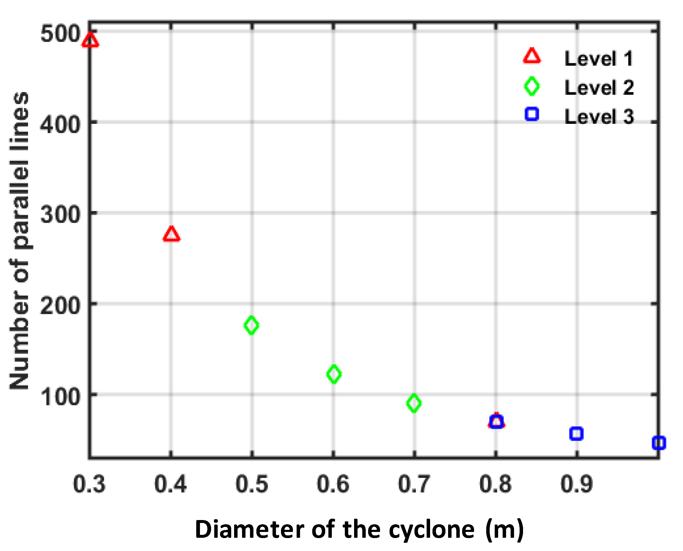
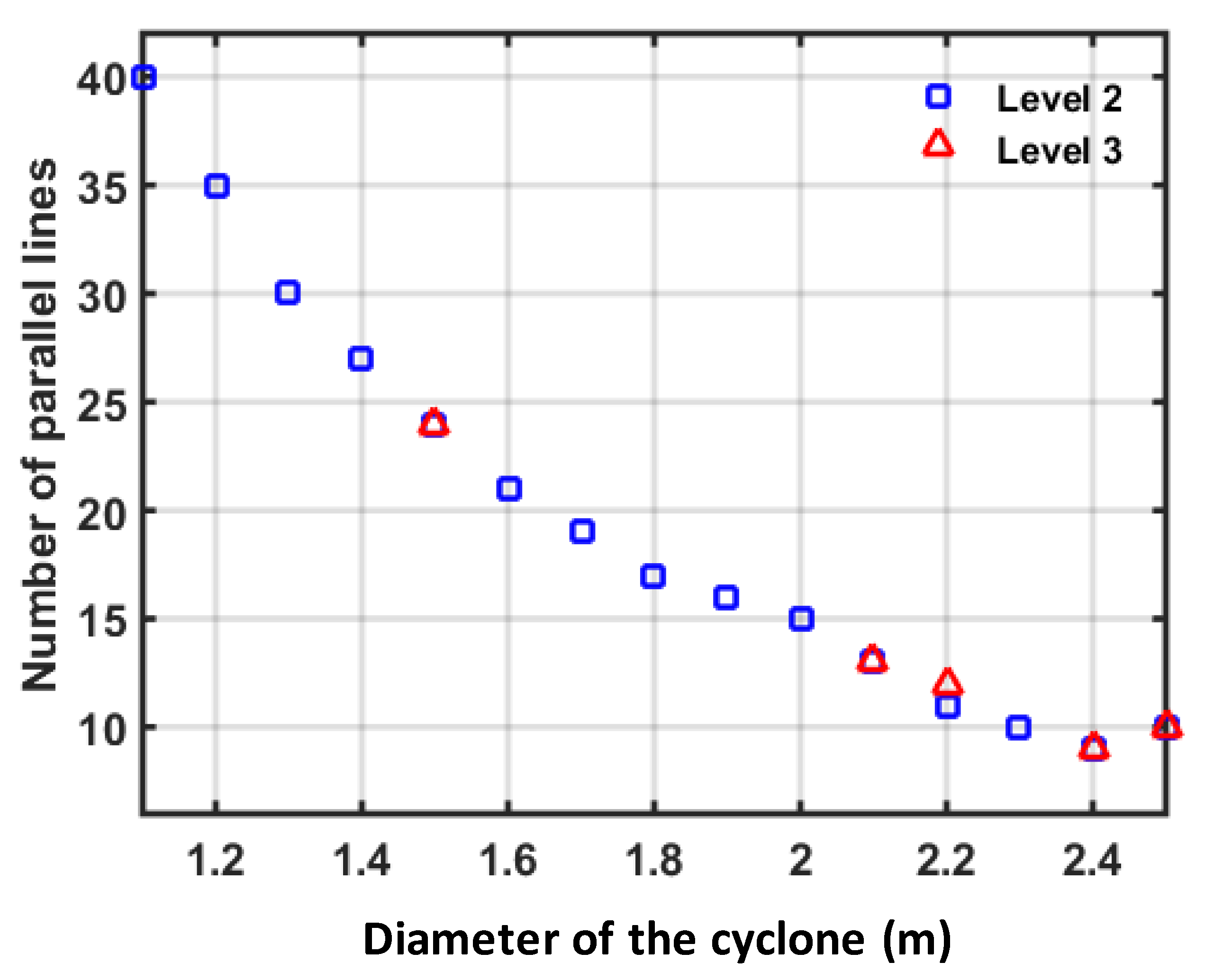
0.3	500	3	0.3	489	0.835	0.201	0.868	30.000	2186.72	0.057

shows some of the results obtained from optimization simulations for different values of bounds used for the decision variables. The effects of varying the upper bound value of decision variables $D_p^U$ and $N_p^U$. in order to find the optimal value of the cyclone diameter and number of parallel lines can also be seen in Figure 5 and Figure 6.

From these figures, while the optimal value of cyclone diameter lies at its upper bound, the optimal solution for the number of parallel lines lies within a wide range of values. These optimal values of D_p and N_p will be used by the optimization process to compute the optimal value of the pressure drop, inlet velocity, and total cost. It should be noted that a certain value of the upper bound of N_p cannot be used in obtaining the feasible solutions for all relaxed NLP sub-problems. For example, the optimal solution is only obtained by GAMS/DICOPT when using $N_p^U=500$ along with the value of 0.3 m as the upper bound of cyclone diameter. As a result, the arrangement of 1D3D–2D2D in series (level 3) is found as the best arrangement with N_p = 489 and of 30 m/s being achieved by the inlet velocity. The resultant value of the total cost for this case is high ($0.057/s) because of the large number of the cyclones (i.e., 489 parallel lines × 2 series cyclone = 978 cyclones) with D_p = 0.3 m. 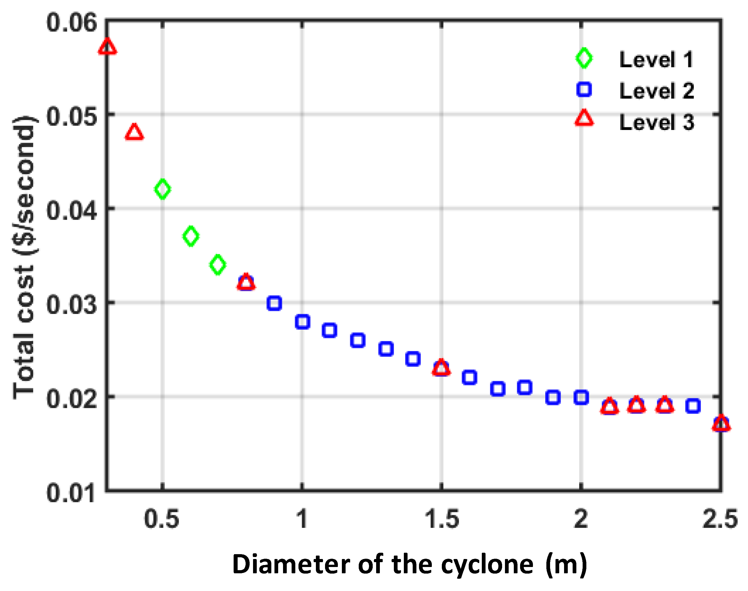Figure 7 shows the relationship between the optimal value of the cyclone diameter and the minimum total cost achieved from the optimization.

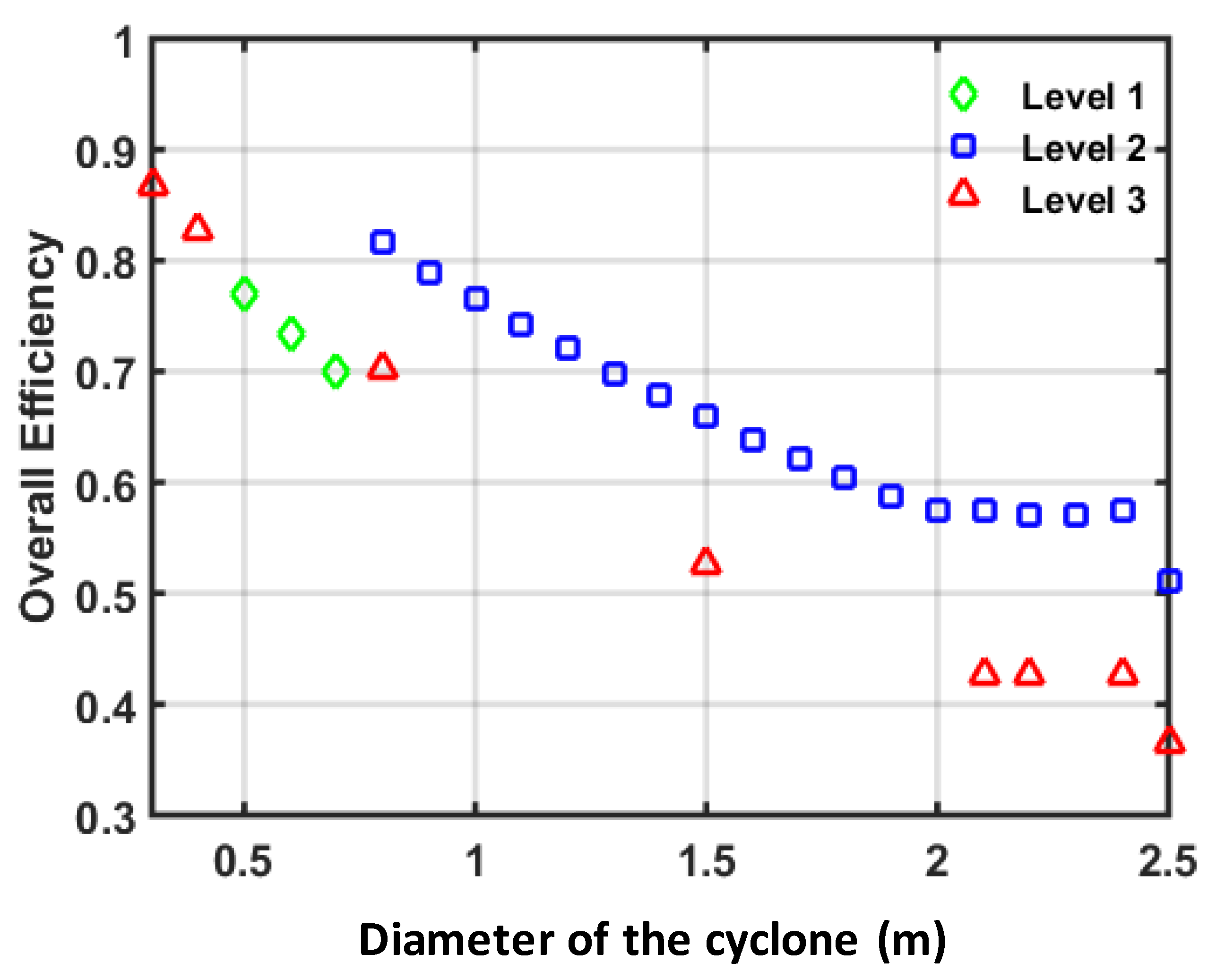
From Figure 7, an increase in the optimal value of D_p will result in a decrease in the total cost c_tot. This is because the operating cost is proportional to $\frac{1}{D^2}$ and even though the capital cost is proportional to diameter of the cyclone, a decreased value of the operating cost tends to be more dominant than the capital cost in obtaining the optimum total cost. The maximum value of the overall efficiency of the cyclone arrangement that can be attained for a certain upper bound of the cyclone diameter is shown in Figure 8. The overall efficiency decreased nonlinearly as cyclone diameter increased with different slope of each level (cyclone arrangement) being chosen. The relationship between the overall efficiency and cyclone diameter in this optimization confirms the same relationship obtained by Faulkner et al. [30], who studied the effects of cyclone diameter on the collection efficiency of 1D3D cyclones.

Moreover, higher collection efficiency is accompanied by an increase in value of the inlet velocity and pressure drop across the cyclone, resulting in a higher total cost. Similar results were also reported by Gimbun et al., 2005. The optimal value of the cyclone pressure drop remains constant for some range of D_p (i.e., D_p = 0.3–0.8 m) since the optimal value of the inlet velocity lies in its upper bound. Thereafter, the trend of cyclone pressure drop will follow a decreasing trend of the inlet velocity as the number of parallel lines (number of cyclones) decreases. The optimum efficiency of the second cyclones would have a lower value than the first cyclone though the dimensions of the second cyclone are the same as the first cyclone. This is due to the fact that the cut size diameter of the second cyclone will increase (due to an increase in the overall efficiency of the first cyclone) to retain the same diameter second cyclone (as given in Equations (16) and (17)). These results are found to be in line with the results reported by Whitelock and Buser [21], who studied the performance of multiple (up to four) 1D3D cyclones arranged in series. It is interesting to observe from Figure 8 that there are only three from four levels available that have been chosen by the model as the best arrangement for a certain value of the decision variables D_p and N_p. For instance, with the resultant value of the efficiency more than 75 %, level 3 (1D3D + 2D2D) is selected as the best cyclone arrangement for D_p = 0.3–0.4 m, level 1 (1D3D + 1D3D) for D_p = 0.5 m, and level 2 (2D2D + 2D2D) for D_p = 0.8–1.0 m. From the whole range, level 1 is available only when the value of D_p is in the range between 0.5 and 0.7 m. Meanwhile, level 2 is found as being more dominant than the others in which it is selected as the best arrangement for a wide range value of the optimum diameter of the cyclone (D_p = 0.8 m to 2.5 m). At a certain point, there are two levels selected as the best arrangement with the same D_p and N_p. For example, the upper bound value of 0.8, 1.5, 2.1, 2.4, and 2.5 m would result in two levels selected (i.e., level 2 and level 3) as the best arrangement with the same optimum number of parallel lines at each D_p. Another result shows that the same two levels are selected as the best arrangement with the same D_p = 2.2 m, but with different value of N_p. The total costs associated with each level (Figure 7) is found to have the same value. Based on these results, two different types of cyclone arrangement can be selected at the same cost but with different efficiencies (Figure 8) where the overall efficiency of cyclone arrangement on level 2 (2D2D + 2D2D) is found to be higher than level 3 (1D3D + 2D2D). To further check the sensitivity of the decision variables to the optimal solutions, an additional optimization was also performed by using all the three decision variables (N, D_p, and η_ov). This optimization is also intended to computationally investigate the effect of η_ov if the bound is changed. In this case, the lower bound for the overall cyclone efficiency (${\eta }_{ov}^L$) is set to have the initial value of 80% and then is increased in increments of 5%. Meanwhile, prior bounds of $N_p^U$ and $D_p^U$ are also selected. The optimal value of cyclone diameter and number of parallel lines for a given constraint of decision variable η_ov should lie within the bounds. Otherwise, a higher value of the upper bound ($D_p^U$ and $N_p^U$) should be applied. The computational results of this optimization are presented in

Table 6. Optimization results using the decision variables N and η_ov.

$D_p^U$	$N_p^U$	${\eta }_{ov}^L$	${\eta }_{ov}^U$	k	Dp	Np	η1	η2	${\eta }_{o{v}_t}$	$v_{i_p}$	∆P	ctot
1	450	0.80	1	3	0.476	194	0.752	0.193	0.80	30	2186.78	0.043
1	450	0.85	1	3	0.344	373	0.813	0.200	0.85	30	2186.78	0.052
2	1000	0.90	1	3	0.226	861	0.875	0.202	0.90	30	2186.78	0.069
1	550	0.90	1	2	0.425	244	0.888	0.110	0.90	30	2186.78	0.046

.

The method selects the lower bound of η_ov as the optimal value. The sensitivity of η_ov to the optimal solutions obtained from this optimization is found to be in accordance with the numerical findings given in Table 5. For instance, as the cyclone diameter decreased along with the optimal value of inlet cyclone remains constant at its upper bound, the overall efficiency will increase. The optimal value of η_ov = 90% obtained in this optimization is higher than the value of the previous optimization (η_ov = 86.8%). It indicates that a higher η_ov is attainable by changing its lower bound until the optimal solution could be reached. From Table 6, the model shows its consistency in selecting the cyclone arrangement of 1D3D + 2D2D (level 3) as the best arrangement to obtain the optimal value of overall efficiency in the range of 80–90%. If these results are combined with the results given in Table 5 (for η_ov > 80%), it will complete the search for the optimal solution of level 3 to attain the maximum value of overall efficiency as presented in

Table 7. Complete results for level 3 as the best arrangement and ${\eta }_{o{v}_t}$ = 80–90%.

k	Dp	Np	η1	η2	${\mathit{\eta }}_{\mathit{o}{\mathit{v}}_{\mathit{t}}}$	${\mathit{v}}_{{\mathit{i}}_{\mathit{p}}}$	∆P	ctot
3	0.476	194	0.752	0.193	0.800	30	2186.78	0.043
3	0.400	275	0.786	0.197	0.828	30	2186.78	0.048
3	0.344	373	0.813	0.200	0.850	30	2186.78	0.052
3	0.300	489	0.835	0.201	0.868	30	2186.78	0.057
3	0.226	861	0.875	0.202	0.900	30	2186.78	0.069

.

However, the optimal solution for η_ov = 90% (Table 6) provides two levels as the best arrangement, i.e., level 2 and 3. The cyclone arrangement of 2D2D + 2D2D (level 2) will have a lower optimum number of parallel lines even though its dimensions are bigger than the cyclone arrangement of 1D3D + 2D2D (level 3). Consequently, the total cost of the cyclone arrangement of 2D2D + 2D2D is lower than the 1D3D + 2D2D, or in other words, the cyclone arrangement of 2D2D + 2D2D is more efficient in the total cost. The optimization results obtained from the present mathematical programming models were also compared with the results from Ravi et al. [11], who studied a multi-objective optimization of a set of N identical reverse-flow cyclone separators in parallel by using the non-dominated sorting genetic algorithm (NSGA). Since they used nine decision variables in the optimization, compared to three decision variables in the present study, not all results would be presented. In particular, only the optimum solution of the number of parallel cyclones, cyclone diameter, and the efficiency of the cyclone are used for comparison.

Table 8. Comparison of the optimal solution of decision variables.

η	Present Study		Ravi et al. [11]
	Number of Cyclones	D (m)	Number of Cyclones	D (m)
77%	352	0.500	1400	0.300
80%	388	0.476	1600	0.300
85%	746	0.344	1300	0.300

shows the comparison of the optimal solution of decision variables, i.e., the number the of cyclone, diameter of the cyclone, and efficiency of the cyclone, where the results were evaluated using the same input feed given in Table 3 and the same range of dimensions ratio of the cyclones (i.e., a₀, b₀, and D_e0). It should be noted that there is no table provided by Ravi et al. [11], all the results are presented in scatter charts instead. Hence, the values listed in Table 8 are rough estimated numbers from those charts provided.

The comparisons illustrated that the present study gave the lower number of parallel cyclones for the same value of the efficiency of the cyclone. In addition, the optimum efficiency of the cyclone that can be achieved from the present study (90%) is slightly higher than Ravi et al. [11]. Based on the above comparisons, it can be concluded that the optimization of the cyclone arrangement in parallel-series using 1D3D and/or 2D2D cyclones found to be a novel solution among other pollution control strategies to reduce the pollution to the minimum level.

4. Conclusions

This study introduced a MINLP (Mixed Integer Nonlinear Programming) model to find the best cyclone arrangement with the optimal number and configuration/dimensions of the cyclone from four combinations of 1D3D and 2D2D cyclones arranged in parallel-series. The cyclone arrangement is optimized with respect to the minimum total cost which includes the operating cost and capital cost. The proposed model is implemented to handle a total flow rate of 165 m³/s of a stream to be processed in a paper mill. It was found that the diameter D is the most important decision variable in the model to obtain the optimal solution. Different values used for the upper bound of D and N resulted in three different cyclone arrangements selected as the optimal solution. It was found that the overall efficiency of the cyclone as well as the optimal number of the cyclone will decrease as the cyclone diameter increases, followed by a decrease in the total cost. As a result of this study, the parallel-series cyclone arrangement of 2D2D + 2D2D was found to be more economical and efficient compared to the others.

References

1. Nakhaei, M.; Lu, B.; Tian, Y.; Wang, W.; Dam-Johansen, K.; Wu, H. CFD modeling of gas–solid cyclone separators at ambient and elevated temperatures. Processes 2020, 8, 228. [Google Scholar] [CrossRef] [Green Version]
2. Zhuge, X.; Qi, X.; Wang, S.; Liu, Y. Evaluation and improvement of the performance of a wellhead multistage bundle gas–liquid separator. Processes 2022, 10, 632. [Google Scholar] [CrossRef]
3. Liu, L.; Dou, H.S.; Chen, X. Effect of particle diameter and injection position on the separation performance of cyclone separators. J. Comput. Multiph. Flows 2016, 8, 40–47. [Google Scholar] [CrossRef]
4. de Souza, F.J.; de Vasconcelos, S.; de Moro Martins, D. Effects of the gas outlet duct length and shape on the performance of cyclone separators. Sep. Purif. Technol. 2015, 142, 90–100. [Google Scholar] [CrossRef]
5. de Souza, F.J.; de Vasconcelos, S.; de Moro Martins, D. Simulation of the performance of small cyclone separators through the use of post cyclones (PoC) and annular overflow ducts. Sep. Purif. Technol. 2015, 142, 71–82. [Google Scholar] [CrossRef]
6. Safikhani, H.; Mehrabian, P. Numerical study of flow field in new cyclone separators. Adv. Powder Technol. 2016, 27, 379–387. [Google Scholar] [CrossRef]
7. Luciano, R.D.; Silva, B.L.; Rosa, L.M.; Meier, H.F. Multi-objective optimization of cyclone separators in series based on computational fluid dynamics. Powder Technol. 2018, 325, 452–466. [Google Scholar] [CrossRef]
8. Abdul-Wahab, S.A.; Failaka, M.F.; Ahmadi, L.; Elkamel, A.; Yetilmezsoy, K. Nonlinear programming optimization of series and parallel cyclone arrangement of NPK fertilizer plants. Powder Technol. 2014, 264, 203–215. [Google Scholar] [CrossRef]
9. Gerrard, A.M.; Liddle, C.J. The optimal choice of multiple cyclones. Powder Technol. 1976, 13, 251–254. [Google Scholar] [CrossRef]
10. Martinez-Benet, J.M.; Casal, J. Optimization of parallel cyclones. Powder Technol. 1984, 38, 217–221. [Google Scholar] [CrossRef]
11. Ravi, G.; Gupta, S.K.; Ray, M.B. Multiobjective optimization of cyclone separators using genetic algorithm. Ind. Eng. Chem. Res. 2000, 39, 4272–4286. [Google Scholar] [CrossRef]
12. Swamee, P.K.; Aggarwal, N.; Bhobhiya, K. Optimum design of cyclone separator. AIChE J. 2009, 55, 2279–2283. [Google Scholar] [CrossRef]
13. Grossmann, I.E. Mixed-integer optimization techniques for algorithmic process synthesis. Adv. Chem. Eng. 1996, 23, 171–246. [Google Scholar] [CrossRef]
14. Grossmann, I.E. Review of nonlinear mixed-integer and disjunctive programming techniques. Optim. Eng. 2002, 3, 227–252. [Google Scholar] [CrossRef]
15. Rosenthal, R.E. GAMS—A User’s Guide; GAMS Development Corporation: Washington, DC, USA, 2007. [Google Scholar]
16. Benitez, J. Process Engineering and Design for Air Pollution Control; Prentice Hall: Englewood Cliffs, DC, USA, 1993. [Google Scholar]
17. Wang, L.; Parnell, C.B.; Shaw, B.W. Performance characteristics of cyclones in cotton-gin dust removal. Agric. Eng. Int. CIGR J. 2002, 4, 1–18. Available online: https://ecommons.cornell.edu/handle/1813/10269 (accessed on 28 October 2022).
18. Wang, L.; Parnell, C.B.; Shaw, B.W.; Lacey, R.E. A theoretical approach for predicting number of turns and cyclone pressure drop. Trans. ASABE 2006, 49, 491–503. [Google Scholar] [CrossRef]
19. Gillum, M.N.; Hughs, S.E.; Armijo, B.M. Use of secondary cyclones for reducing gin emissions. Trans. ASAE 1982, 25, 210–213. [Google Scholar] [CrossRef]
20. Columbus, E.P. Series cyclone arrangements to reduce gin emissions. Trans. ASABE 1993, 36, 545–550. [Google Scholar] [CrossRef]
21. Whitelock, D.P.; Buser, M.D. Multiple series cyclones for high particulate matter concentrations. Appl. Eng. Agric. 2007, 23, 131–136. [Google Scholar] [CrossRef] [Green Version]
22. Wang, L.; Parnell, C.B.; Shaw, B.W.; Lacey, R.E. Analysis of Cyclone Collection Efficiency. In Proceedings of the 2003 ASAE Annual International Meeting, Las Vegas, NE, USA, 27–30 July 2003; p. 034114. [Google Scholar] [CrossRef]
23. Clift, R.; Grace, J.R.; Weber, M.E. Bubbles, Drops, and Particles, Courier Corporation; Dover Publications: Mineola, NY, USA, 2005. [Google Scholar]
24. Sinnott, R.K. Chemical Engineering Design, 4th ed.; Elsevier Butterworth-Heinemann: Oxford, UK, 2005; Volume 6. [Google Scholar]
25. Gimbun, J.; Chuah, T.G.; Choong, T.S.Y.; Fakhru’l-Razi, A. A CFD study on the prediction of cyclone collection efficiency. Int. J. Comput. Methods Eng. 2005, 6, 161–168. [Google Scholar] [CrossRef]
26. Shepherd, C.B.; Lapple, C.E. Air Pollution Control: A Design Approach. Cyclones, 2nd ed.; Waveland Press Inc.: Long Grove, IL, USA, 1939. [Google Scholar]
27. Grossmann, I.E.; Viswanathan, J.; Veccheitti, A.; Raman, R.; Kalvelagen, E. GAMS/DICOPT Solver Description; GAMS Corporation Inc.: Frechen, Germany, 2003. [Google Scholar]
28. Viswanathan, J.; Grossmann, I.E. A combined penalty function and outer-approximation method for MINLP optimization. Comput. Chem. Eng. 1990, 14, 769–782. [Google Scholar] [CrossRef]
29. Bhaskar, V.; Gupta, S.K.; Ray, A.K. Applications of multiobjective optimization in chemical engineering. Rev. Chem. Eng. 2000, 16, 1–54. [Google Scholar] [CrossRef]
30. Faulkner, W.B.; Buser, M.D.; Whitelock, D.P.; Shaw, B.W. Effects of cyclone diameter on performance of 1D3D cyclones: Collection efficiency. Trans. ASABE 2007, 50, 1053–1059. [Google Scholar] [CrossRef]
Figure 1. Schematic of the cyclone and the design specification dimensions of the cyclone.
Atmosphere 13 01831 g001
Figure 2. Parallel-series cyclone configuration with four levels.
Atmosphere 13 01831 g002
Figure 4. Efficiency versus the cut-size diameter for (a) first cyclone and (b) second cyclone.
Atmosphere 13 01831 g004
Figure 5. Optimal value of number of parallel lines versus diameter of cyclone 1.
Atmosphere 13 01831 g005
Figure 6. Optimal value of number of parallel lines versus diameter of cyclone 2.
Atmosphere 13 01831 g006
Figure 7. Total cost versus diameter of the cyclone.
Atmosphere 13 01831 g007
Figure 8. Optimal value of the overall efficiency vs diameter of the cyclone.
Atmosphere 13 01831 g008