Analog Ensemble Forecasting System for Low-Visibility Conditions over the Main Airports of Morocco

Abstract

Low-visibility conditions (LVC) are a common cause of air traffic, road, and sailing fatalities. Forecasting those conditions is an arduous challenge for weather forecasters all over the world. In this work, a new decision support system is developed based on an analog ensemble (AnEn) method to predict LVC over 15 airports of Morocco for 24 forecast hours. Hourly forecasts from the AROME model of eight predictors were used to select the skillful analogs from 2016 to 2018. The verified hourly observations were used as members of the ensemble. The developed ensemble prediction system (EPS) was assessed over 1 year (2019) as a single-value forecast and as a probabilistic forecast. Results analysis shows that AnEn outperforms persistence and its best performances are perceived generally during night and early-morning lead times. From continuous verification analysis, AnEn forecasting errors are found to be location- and lead-time-dependent and become higher for low-visibility cases. AnEn draws an averaged Centered Root Mean Square Error of about 1500 m for all visibilities, 2000 m for fog and 1500 m for mist. As an EPS, AnEn is under-dispersive for all lead times and draws a positive bias for fog and mist events. For probabilistic verification analysis, AnEn visibility forecasts are converted to binary occurrences depending on a set of thresholds from 200 m to 6000 m by a step of 200 m. It is found that the averaged Heidke Skill Score for AnEn is 0.65 for all thresholds. However, AnEn performance generally becomes weaker for fog or mist events prediction.

1. Introduction

Low-visibility conditions (LVC) have often been responsible for air, land and marine traffic disasters. Regarding the high complexity of boundary layer meteorological processes, forecasting reduced visibility conditions remains a challenging matter for the forecaster community. The occurrence of such conditions leads to multiple risky scenarios, causing accidents in roads, airport terminals, and harbors [1]).

For instance, a dense fog (visibility below or equal to 200 m) that occurred in December 2013 caused several vehicle collisions and fatalities on a highway of the Grand-Casablanca region, Morocco [2]. In the same way, another fog event led to the diversion of 21 aircraft in 2008 at Mohamed V international airport, Casablanca, Morocco [3]. Such diversions result in many economical losses (additional fuel consumption, flight delays, passenger support, etc.) [4]. Furthermore, in reference to the Federal Highway Administration, United States of America, every year fog causes around 25,500 crashes resulting in over 8500 injuries and over 460 deaths all over the USA [5]. Several challenges impede visibility forecasting systems, such as: (a) the high cost of visibility-observing systems and their implementation being restricted to few locations (airports most of the time); (b) the low density of visibility sensors over fog-prone locations; and (c) a limited understanding of the complex interaction between the physical processes leading to low-visibility conditions (fog or mist). All these tragedies and challenges construct a powerful motivation to develop new decision support systems for improving low-visibility conditions forecasting.

Researchers have already used numerical weather prediction (NWP) models to diagnose low-visibility conditions from a set of prognostic weather parameters. Some formulations, such as the Kunkel [6] and Gultepe [7,8] formulas, are widely used to calculate visibility from liquid water content only for the former, and from liquid water content and droplet number concentration for the latter [7,9,10,11,12]. However, previous studies show the limitations of such an approach, which over-/underestimates visibility depending on environmental conditions. As an alternative, many statistical-based forecasting models and data-driven methods have been also explored: fuzzy logic (e.g., [13]), artificial neural networks (ANN) (e.g., [14]), and decision-tree-based methods (e.g., [15]).

Fuzzy logic [13,16,17] has already been applied to visibility forecasting; however, this method’s rules are often complex or have high subjectivity. In the same way, artificial neural networks have been widely used to predict visibility and produce returns-promoting results [14,18,19,20,21]. For instance, the authors in [22] used ANN to predict low-visibility procedure conditions (LVP) at Mohamed V international airport in Casablanca, Morocco. The authors found that ANNs were able to predict LVP conditions and were less sensitive to the LVP type being predicted (fog LVP and no-fog LVP). In addition, ANN was used to predict visibility at Urumqi International Airport [23] and the authors found an absolute mean error of 325 m for fog events. In [15], the authors explored multiple decision-tree-based algorithms to predict visibility over 36 weather stations of Morocco. The authors underline the high potential of decision tree algorithms to improve visibility forecasting compared with persistence and Kunkel’s empirical formula [6], with root mean square error (RMSE) values around 2090 m and a bias of −144 m.

Most of the previous research works were designed to produce a single-value forecast of visibility. From an operational perspective, more visibility forecast scenarios are solicited to cover the whole spectrum of visibility and match the operational procedures. Ensemble methods fill this need by providing a variety of forecast scenarios and hence more agility for deciders. In [24], the authors developed an ensemble forecasting system based on initial conditions perturbation via the breeding vectors technique, in order to predict fog over 13 cities of China and up to 36 h ahead. The authors found that the multivariable-based fog diagnostic method has a much higher detection capability than the approach based only on liquid water content. In line with ensemble forecasting philosophy, the authors in [25] used a multiphysics ensemble where members are constructed via perturbing either initial conditions, physical parameterization, or both to predict visibility. The latter shows that fog prediction from multiphysics ensemble is increased during night and morning hours. The results from this latter show the high variability of findings in terms of topography. The authors also suggest a probabilistic adjustment to reduce complexity and thus to ameliorate EPS performance. Despite the evidence of good ensemble system performance and skill in forecasting LVC, these methods remain very expensive in terms of computational capacity and operational time.

The analog ensemble method is considered as one of the most low cost and intuitive ensemble methods. The author in [13], suggests an analog ensemble based application to forecast ceiling and visibility in 190 Canadian airports where analog similarity is measured using a fuzzy logic distance. The author compared application’s results to persistence and terminal aerodrome forecasts(TAFs). The developed approach draws a Heidke Skill Score (HSS) of up to 0.56 and reveals high performances compared to the chosen benchmarks. On the other hand, the authors in [26] combined a fuzzy-logic-based analog with NWP model predictions to develop a new hybrid forecasting method producing deterministic visibility forecasts. The authors suggest that applying a new weighting strategy to the predictors highly improved the performance of visibility forecasting. The hybrid method surpasses TAFs and results in an HSS of 0.65 for reduced visibility conditions.

Based on the literature review, additional research efforts are required to develop more accurate and better-performing LVC forecasting systems. The main goal of this work is to develop a computationally cheap ensemble forecasting system to predict low-visibility conditions either as a single-value forecast of visibility or as probabilistic prediction where visibility forecasts are converted to binary event probabilities and hence reflect the occurrence or not of low-visibility events depending on a set of visibility operational thresholds. To achieve this purpose, we will be using the analog ensemble method [27]. We focus on the assessment of fog and mist events. It is important to mention that this work is the first AnEn application using the meso-scale operational model AROME [28] for horizontal visibility forecasting near the surface. This model is widely used among an important part of the scientific community, and it is also used operationally in many countries, including Morocco [29].

This paper will be organized as follows: Section 2 describes the used data and study domain. Section 3 describes the used methodology, including AnEn metrics optimization and weighting strategy. Section 4 displays the results. Section 5 is reserved for discussion. Finally, a conclusion and perspectives for further research are provided in Section 6.

2. Data

For this study, hourly observations and forecasts datasets from 2016 to 2019 have been used. Forecasts are provided by the meso-scale model AROME [28] with a resolution of 2.5 km and 90 vertical levels, the first level starting at about 5 m. These were extracted at the nearest grid point from the observation. From this dataset, eight predictor forecasts are used: temperature and relative humidity at 2 m (T2m, RH2m), wind speed and direction at 10 m (WS10m, WD10m), surface and mean sea level pressures (SURFP and MSLP), and liquid water content at 2 m and 5 m (LWC2m, LWC5m). The choice of predictors was determined by two main criteria: (i) data availability, and (ii) physical link with the target variable (visibility). It should be noted that AROME uses twelve 3D prognostic variables: two components of the horizontal wind (U and V), temperature T, the specific content of water vapor $q_v$, rain $q_r$, snow $q_s$, graupel $q_g$, cloud droplets $q_c$, ice crystals $q_i$, turbulent kinetic energy $TKE$, and two non hydrostatic variables that are related to pressure and vertical momentum [28]. AROME also uses the one-moment microphysical scheme ICE3, which is a microphysical parameterization with a fixed cloud droplet concentration ($N_c$ = 300 ${\mathrm{cm}}^{-3}$ over the land and $N_c$ = 100 ${\mathrm{cm}}^{-3}$ over the sea).

Regarding the observation dataset, we use historical hourly visibilities from airport observations (routine aviation weather reports (METARs)) as used in many previous research works, such as [13], using a fuzzy-logic-based analog forecasting system for detecting ceiling and visibility over Canada, Ref. [30] using an analogue dynamical model for forecasting fog-induced visibility over India, and [26] using a fuzzy-logic-based analogue forecasting and hybrid model of horizontal visibility over Hungary. This METAR-based approach could be used worldwide for operation in other airports [31]. The used visibility is measured either by transmissometers or scatterometers depending on the studied airport category (CAT-II or CAT-III). 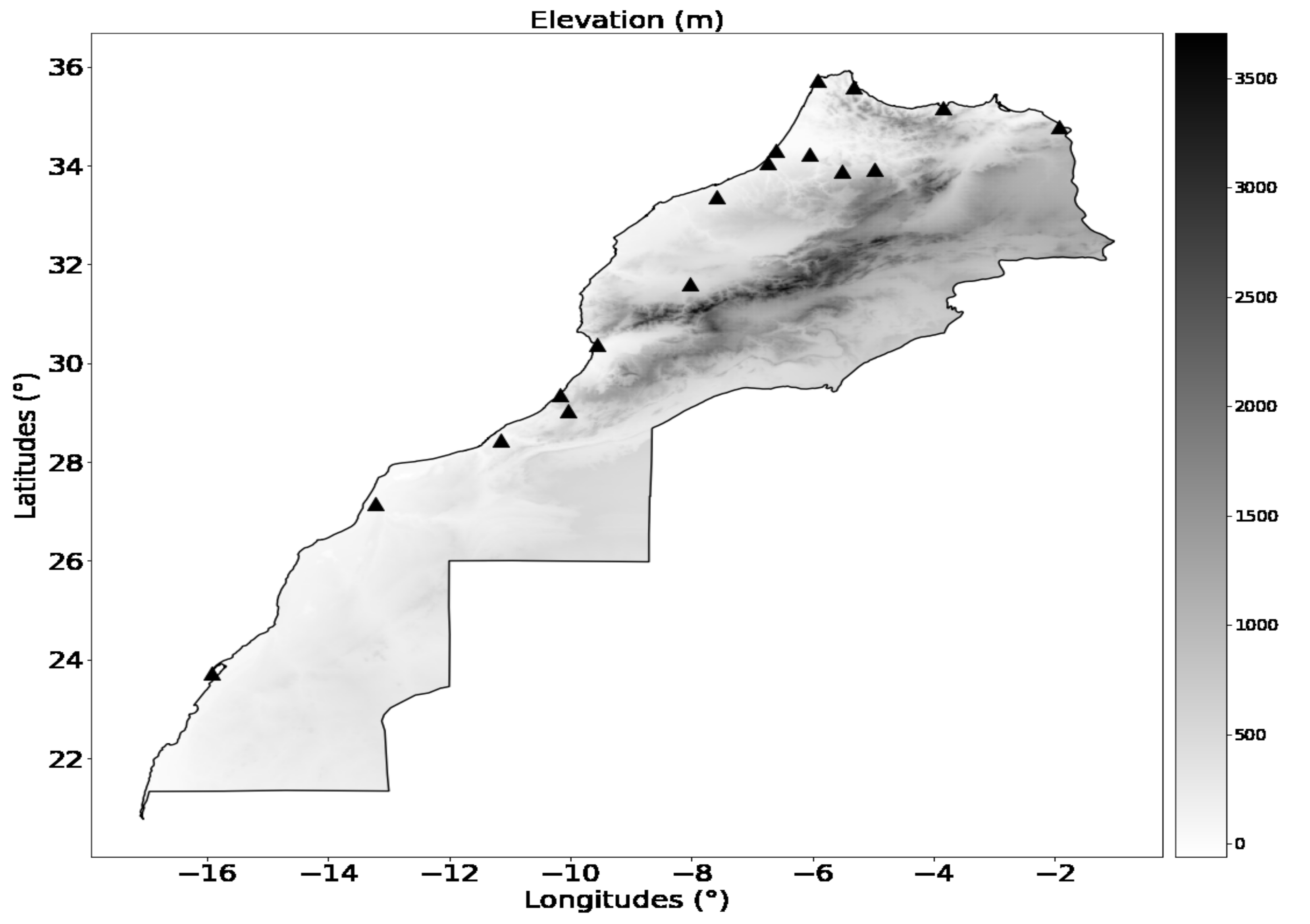In a few airports (CAT-I), the observed visibility represents the shortest horizontal visible distance considering all directions and is estimated by observers in reference to landmarks at airports terminals [32]. Moreover, data are gathered from 17 stations (airports operating 24H/24H), representing different geographic and climatic zones across the Moroccan Kingdom. Figure 1 displays a map positioning each of the studied locations. The training period for AnEn extends from 2016 to 2018 and the 2019 year is used as a verification-independent period.

3. Methods

In this study, different analog ensemble configurations have been tested and evaluated in order to set up a new low-visibility condition forecasting system with a 24 h projection period. Forecast timings of significant changes in flight conditions are supposed to be accurate to within 1 h. Thus, one hour was chosen as a base time step of verification due to the time step of the dynamic model output, and the visibility values were handled as characterizing instantaneous values of a given time. This procedure is maintained for each forecast to preserve comparability. Consequently, very short fogs (lasting below one hour) occurring between two consecutive hours are not taken into account in this study. Thus, in this section, we describe the analog ensemble scheme and also the experimental set up. Indeed, focus has been placed on target output value (weighted average mean, best quantile-based value, and ensemble mean) and the target type (continuous or categorical). In addition, the sensitivity to the threshold of the low-visibility conditions (fog (<1000 m) or mist (≥1000 m and <5000 m)) has been assessed. The persistence-based model is used as a benchmark and its predicted visibility today for a given hour is the same as that which occurred and was observed yesterday at the same time.

3.1. Experiments and Implementation

We first define an occurrence of low-visibility conditions (LVC) at a specific hour when visibility is lower than a predefined threshold. All the forecasted/observed visibilities above the threshold are considered as non-occurrences. In this framework, the experiments described in

Table 1. Experimental setup description.

Parameters	Experiment Details
Training period	2016–2018
Testing and verification period	2019
Locations	17 synoptic airports of Morocco
NWP model	AROME cycle 41, 2.5 km, 90 vertical levels
EPS technique	Analog ensemble [27]
Dataset sampling	24 hourly observations and forecasts
Features	T2m, RH2m, WS10m, WD10m, LWC2m, LWC5m, SURFP and MSLP
Time window	±3 h
Day window	±30 days
Configuration	Continuous visibility and then converted to a binary threshold-based event
Target output value	AnEn mean/weighted average mean/best quantile-based value
Benchmark	Persistence

are performed. Since we are dealing with threshold-based events, the visibility target is treated as a single-value forecast variable by AnEn then converted to probabilistic forecasts of LVC depending on a predefined threshold. In most cases, large values of visibility in a clear sky could induce large bias and error values for the ensemble mean of the EPS. To overcome this issue, all visibilities above 10 km were adjusted to a constant value of 10 km.

3.2. Analog Ensemble Algorithm

In this section, we will first discuss the analog ensemble algorithm as it was introduced by the authors in [27]. The simple idea behind the analog ensemble method is to search past forecast archives for all similar weather situations to the current forecast. This search is based on a set of predictors and a similarity metric presented in Equation (1). Once the most analogous situations are defined, their ground truth observations are used to construct the ensemble members. For our study, we use a slightly changed version of the analog similarity measure in [27]. Predictor weights are defined according to their importance coefficient resulting from stepwise forward selection. We run the latter over the training period. Our predictor set extends to the forecasted T2M, RH2M, WS10M, WD10M, MSLP, SURFP, LWC2M and LWC5M, while the prediction is the observed visibility over the same period. The stepwise forward selection algorithm assigns a coefficient to each predictor depending on its importance and correlation with the observed visibility. Once the coefficients are defined, a normalization process is performed in such a way that the sum of the weights is equal to 1.

The similarity measure used in [27] is defined as follow:

$$∥{\mathbf{F}}_t,{\mathbf{A}}_{t^{\prime }}∥=\sum _{i=1}^{N_{\nu }}\frac{w_i}{{\sigma }_i}\sqrt{\sum _{j=-\tilde{t}}^{\tilde{t}}{(F_{i,t+j}-A_{i,t^{\prime }+j})}^2}$$

(1)

where $F_t$ is the current NWP deterministic forecast valid at the future time t at a station location; $A_{t^{\prime }}$ is an analog (past forecast) at the same location and with the same forecast lead time but valid at a past time t’; $N_{\nu }$ and $w_i$ are the number of physical variables used in the analog search and for their weights, respectively; ${\sigma }_i$ is the standard deviation of the time series of past forecasts of a given variable i at the same location and forecast lead time; $\tilde{t}$ is equal to half the number of additional times over which the metric is computed; and $F_{i,t+j}$ and $A_{i,t^{\prime }+j}$ are the values of the forecast and the analog in a time window with j from −t to +t for a given variable i.

3.3. Analog Ensemble Weighted Mean

During the analog selection process, an analog may come from any past date within the training period (e.g., a day, week, or several months ago). Then, the analog quality (skill) is determined using the distance between the analog “A” and the target forecast “F” (Equation (1)) and the N analogs with the smallest distance to “F” are selected and sorted. Thus, the verified observations (O) associated with the time occurrences of the analog forecasts (A) are selected to form the analog ensemble. The analog ensemble weighted mean (AnEn) can be used for deterministic prediction and is computed as the weighted average value of the ensemble [33,34]. The weight associated with each member in the ensemble is proportional to the inverse of the distance in Equation (1) and can be calculated as follows:

$$w_{i,t}=\frac{1}{∥{\mathbf{F}}_t,{\mathbf{A}}_{t^{\prime }}∥}$$

As a consequence, the analog ensemble weighted mean is equal to

$$AnE{n}_{t,weighted.mean}={\delta }_t*\sum _{i=1}^M{w}_{i,t}*m_{i,t};$$

where ${\delta }_t={\sum }_{i=1}^M{w}_{i,t}$, M is the total number of members (=25), and $m_{i,t}$ is the ith ensemble member at lead time t.

3.4. Best Quantile of the Analog Ensemble

In this study, the method in reference [26] is used to find the ensemble quantile with the best probabilistic score. Indeed, the authors used the Heidke Skill Score (HSS) as a measure of the performance of each algorithm relative to random chance (see the HSS formulation in Appendix A). In addition, this score remains acceptable during the verification of rare events, which is in line with low-visibility conditions. In accordance with aviation practice, which applies different operational visibility thresholds, the visibility categories are represented by the upper limit of the given category. In fact, different rules or flight procedures must be applied when the visibility drops below a given threshold (limit). In this study, the thresholds vary from 200 m to 6000 m by a step of 200 m. For each threshold, the HSS score is computed for each quantile from 5% to 95% by a step of 5%. Then, for each quantile, the average value of the score is calculated over all airports, all thresholds, and all lead times. In Figure 2, the evolution of the HSS score and the incorrect forecasts is plotted for three cases (whole year, fog events, and mist events) as a function of the quantiles (from 5% to 95%). By the definition of this score, the best quantile is the one that maximizes the HSS and minimizes the incorrect forecasts (Missed + False Alarms), which includes the false alarms and the missed cases. It is seen clearly that the quantile of 30% is the optimum one and is therefore used in this study.

4. Results Analysis

In this section, the analysis of the results is performed from two points of view. First, the horizontal visibility forecasting is treated as a single-value forecast of the analog ensemble system (AnEn mean, AnEn weighted mean, and AnEn quantile 30%). In this framework, the performance of AnEn is assessed using the bias, RMSE, centered RMSE (CRMSE), and correlation coefficient (CC) (for more details on their definition and formulation, see Appendix A). These verification metrics are chosen to reveal the levels of systematic and random error in the forecasts. Second, the low-visibility conditions are treated as binary events and the output of AnEn is assessed as a probabilistic ensemble forecast (spread–error relationship, statistical consistency, reliability, resolution, and HSS).

4.1. Ensemble Statistical Consistency

An especially important aspect of ensemble forecasting is its capacity to yield information about the magnitude and nature of the uncertainty in a forecast. While dispersion describes the climatological range of an ensemble forecast system relative to the range of the observed outcomes, ensemble spread is used to describe the range of outcomes in a specific forecast from an ensemble system. In fact, as an ensemble forecast, the developed forecasting system must be statistically consistent with the observation. In fact, the AnEn members must be indistinguishable from the truth (i.e., the PDFs from which the members and the truth are drawn must be consistent [35]). This statistical consistency is assessed in this study using the spread–error diagram and the rank histogram.

4.1.1. Spread–Error Relationship

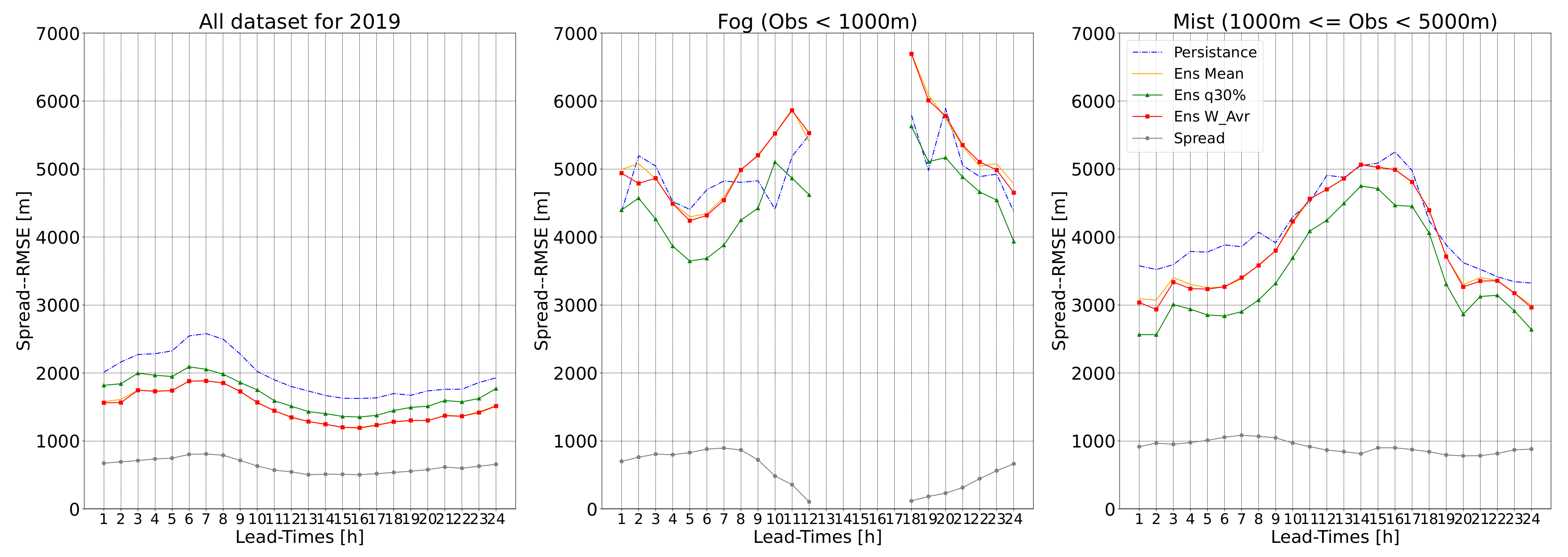
The spread–error relationship is a commonly used plot for ensemble dispersion verification. In Figure 3, we exhibit the ensemble spread against the RMSE of the ensemble mean forecasts for three cases: the whole dataset, fog events, and mist events. The closeness between RMSE and spread reveals the degree of consistency; hence, if the RMSE curve is below the spread curve then the ensemble is considered over-dispersive, and for the inverse case the ensemble is considered under-dispersive. Thus, for the whole dataset, AnEn seems consistent since the RMSE and spread curves are close. Nonetheless, for fog and mist events, AnEn is under-dispersive, especially for night lead times (18 h–6 h) for fog and for all the lead times in the case of mist. In all cases, RMSE is above spread, which means that AnEn is under-dispersive. In addition, the spread is too small which means that the developed ensemble prediction system did not simulate some sources of error. In general, one would expect that larger ensemble dispersion implies more uncertainty in the forecast, and that the inverse is also true.

4.1.2. Rank Histogram

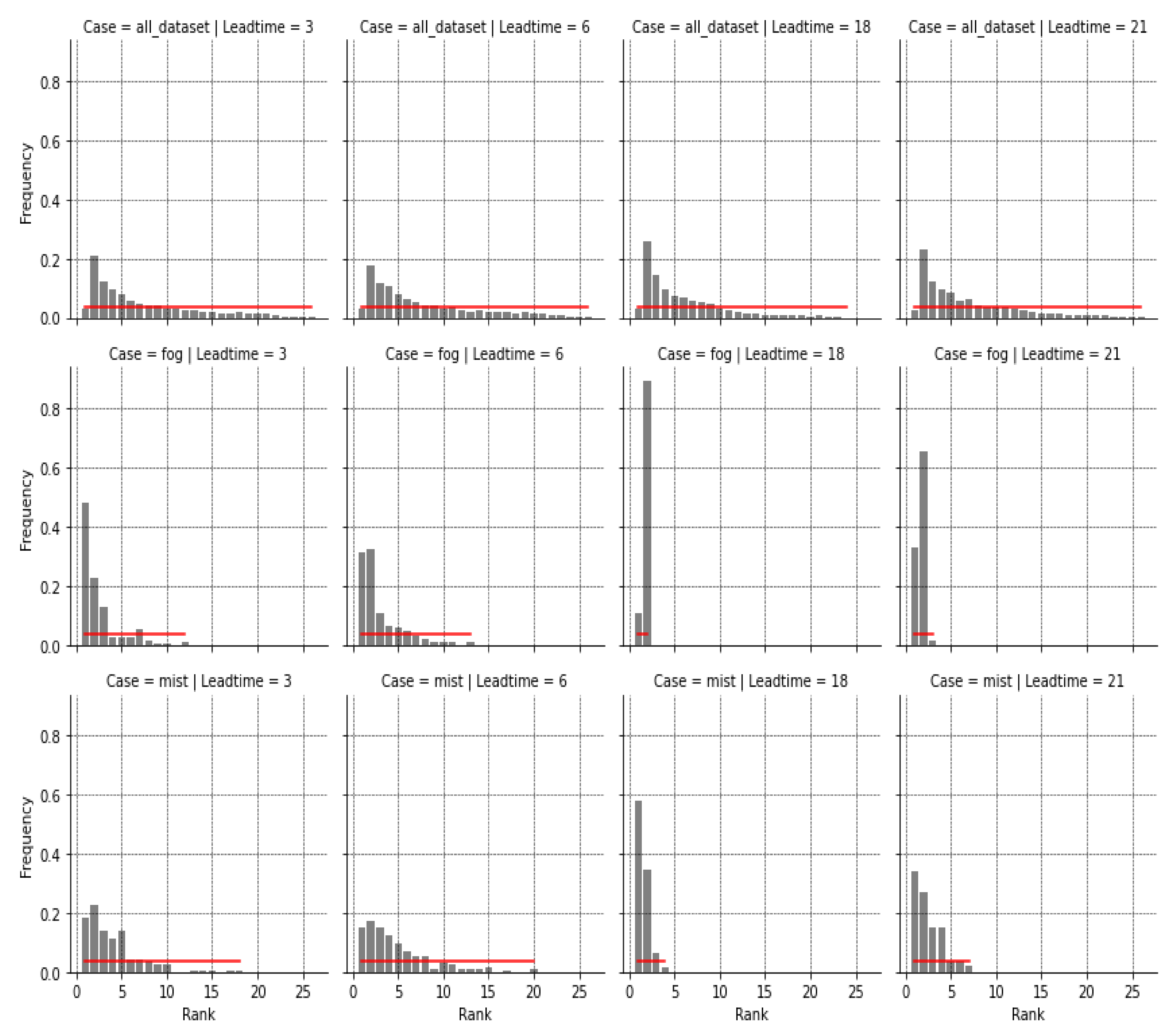
Rank histogram is a method for checking where observations fall with respect to ensemble forecasts. This gives an idea about ensemble dispersion and bias. For an ensemble with perfect spread, each member represents an equally probable possibility; hence, observation is equally likely to fall between any two members. In Figure 4, we display the rank histograms for 3 h, 6 h, 18 h, and 21 h lead times. In general, AnEn represents a left-skewed rank histogram which is translated as a positive bias (the observed visibility often being lower than all AnEn members).

Overall, it is demonstrated that AnEn is under-dispersive with a positive bias. In addition, the best quantile of AnEn outperforms the other configurations for low-visibility conditions (<5000 m).

4.2. Continuous Verification Analysis (Bias, RMSE, CRMSE, and CC)

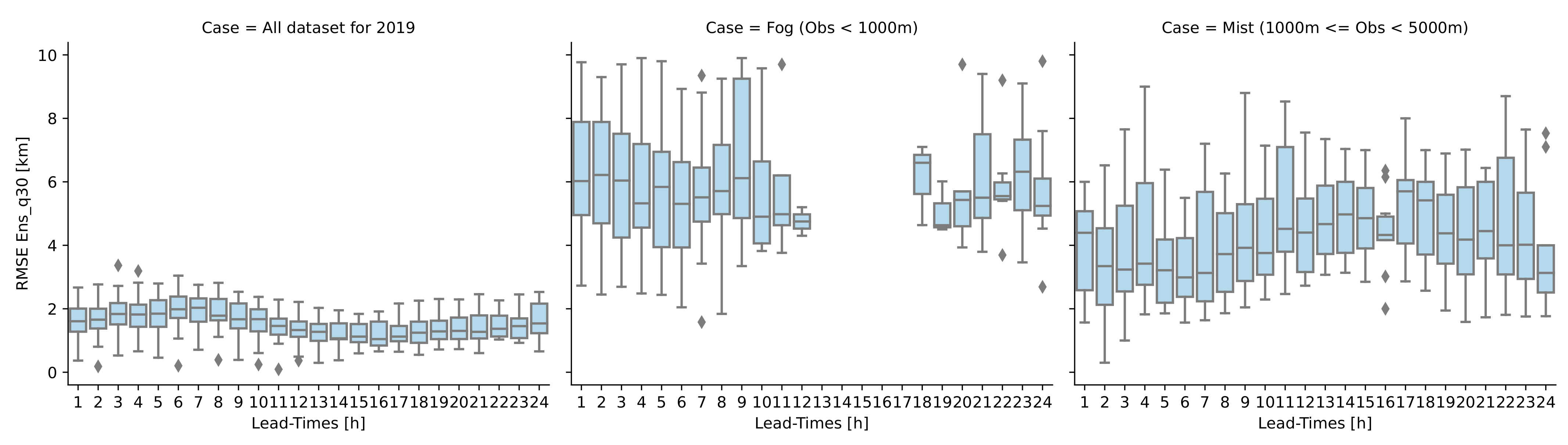
Figure 5 displays the RMSE boxplots of the best quantile of AnEn as a function of lead time for all locations. Each boxplot gathers RMS error values for each of the studied airports. For the whole year 2019, the error spatial variability is very small around a median of 2000 m. This reflects good agreements overall between stations due to the predominance of good visibilities over the testing period. Nevertheless, the best quantile of AnEn shows high RMS error medians when dealing with fog and mist conditions (6000 m and 4500 m, respectively). This points out the high variability and sensitivity of AnEn performances to lead time and geographical position. In the following, we will delve deeper into continuous visibility forecast verification in order to reveal the levels of systematic and random error in the forecasts. To achieve this, the lead time performance of AnEn is assessed by comparing the three configurations of AnEn (AnEn mean, AnEn weighted mean, and AnEn quantile 30%) and also persistence in terms of bias, CRMSE, and coefficient of correlation (Figure 6).

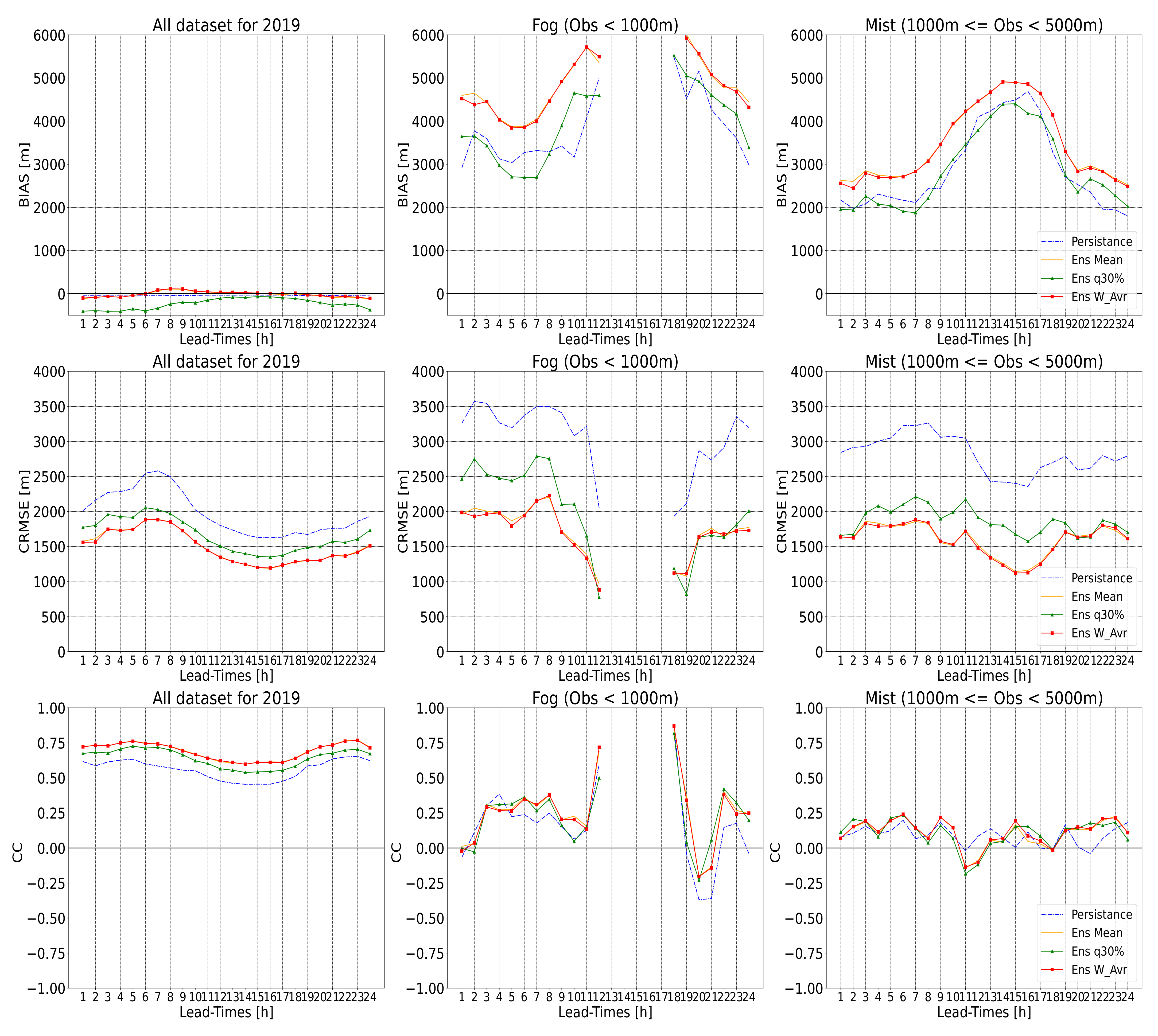
In Figure 6, and all subsequent plots, we display scores for three cases over the whole year of 2019: (a) for all visibilities, (b) for fog events (where visibility < 1000 m), and (c) for mist events (where 1000 m <= visibility < 5000 m). For all visibilities over the testing period (2019), AnEn ensemble mean and AnEn weighted average show the lowest bias close to the reference line of zero, similarly to persistence, while AnEn quantile 30 slightly underestimates the predicted value of horizontal visibility (bias reached −400 m). This could be explained by the predominance of good visibilities during the year. However, we are interested in low-visibility conditions. Thus, for fog events, the AnEn quantile 30% overestimates visibility and displays the lowest bias values (about 2600 m in the morning). It should be noted that fog phenomena were not observed during the daytime at all the studied airports over the whole year of 2019. For mist events, persistence and AnEn quantile 30% display the lowest bias (positive), with tiny differences in magnitude. The bias shows a diurnal variability, where it jumps from 2000 m during the night to 4500 m during the daytime.

AnEn configurations (mean, weighted mean, and quantile 30%) display a better CRMSE than persistence for all cases of low-visibility conditions (fog and mist). When removing bias from forecasts, the AnEn quantile 30% is outperformed by the AnEn mean and weighted average in terms of CRMSE for fog and mist cases. For the whole test period, AnEn quantile 30% shows an error close in magnitude to the AnEn mean and weighted average (Figure 6).

Regarding the correlation between the predicted visibility and the observed one for the whole-year 2019 dataset, AnEn forecasts are highly correlated with observation with an average CC around 0.7 over all lead times for all visibilities over 2019, surpassing the persistence (CC = 0.6). However, once considering rare events (visibility below 5000 m), the correlation becomes weaker and drops to 0.4 for fog events and 0.2 or less for mist events. When combining bias, CC, and CRMSE results, the RMS error for all visibilities over the whole year 2019 is mainly produced by random errors since correlation for the whole dataset is above 0.6 and the magnitude of CRMSE is greater than that of bias. Nonetheless, for low-visibility conditions (fog and mist), we found lower CC values (below 0.5) associated with errors that are mainly systematic (the magnitude of CRMSE is lower than that of bias).

In taking the ensemble mean or the ensemble weighted mean, one filters the unpredictable components of the forecast. Thus, the filtered forecast will be smoother (more like a climatology) and consequently will have a smaller error. On the other hand, systematic errors are predictable and tend to happen frequently, while random errors are unpredictable and relatively uncontrollable. Bias correction is a way to address systematic error by accounting and adjusting for a known bias. This point is out of the scope of this study.

4.3. Probabilistic Forecast Verification (Reliability, Resolution, and Performance)

Overall, it is demonstrated that it is quite difficult to predict low-visibility conditions (<5000 m) using the AnEn value (AnEn mean, AnEn weighted mean, and AnEn quantile 30) as a single-value forecast. This could be due to many factors, such as the measurement principle of the observed visibilities. In fact, visibility represents the shortest horizontal visible distance considering all directions [32] and is traditionally measured by human observers using landmarks around weather stations. This is still widely carried out, even if it is more common now to use visibility sensors to produce automatic observations of visibility, especially at airports [1]. Each station has a list of objects suitable for both daytime observations (towers, buildings, trees, etc.) and nighttime observations (light sources) at known distances from the station. Thus, the horizontal visibility is typically classified, but the employed classes vary from place to place. Therefore, using the probabilistic ensemble forecasting based on AnEn is a good alternative to predict low-visibility conditions as a binary event (occurrence/non-occurrence). This point is treated in detail in this section.

4.3.1. Reliability

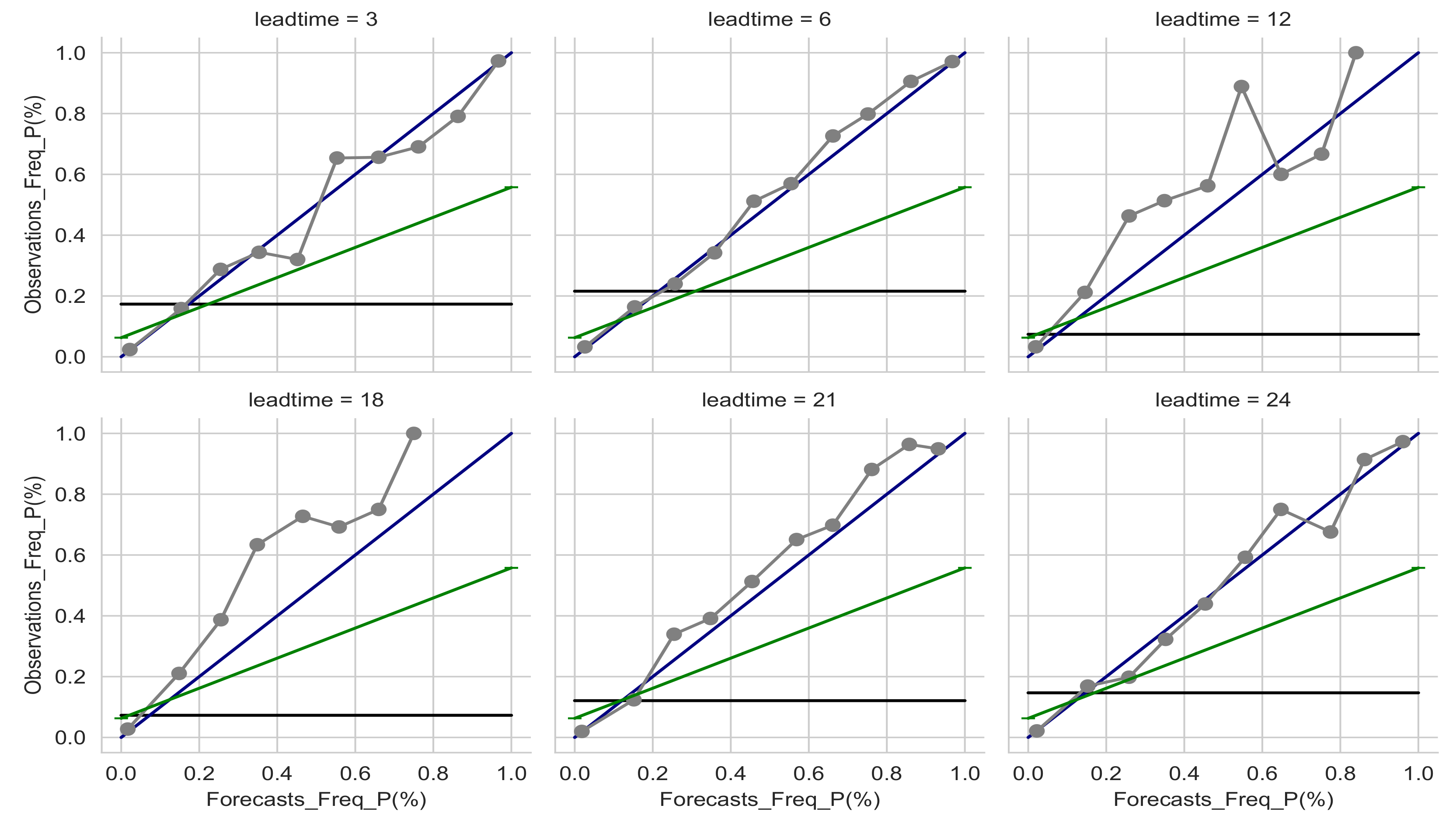
Reliability translates the average agreement between observations and forecasts. A good indicator of ensemble reliability is the reliability diagram shown in Figure 7 for visibilities below 5000 m. In this figure, the observed frequencies are plotted against forecast probabilities for low visibilities at some selected lead times (3 h, 6 h, 12 h, 18 h, 21 h, and 24 h). Reliability is indicated by the closeness of the plotted curve to the diagonal, which refers to perfect reliability. Any deviation of the curve from the reference line is considered as a conditional bias of the ensemble system. For night lead times (3 h, 6 h, 21 h, and 24 h), AnEn exhibits good reliability since the reliability curve is close to the perfect reliability line. Nevertheless, for 12 h and 18 h, the reliability curve is above the reference line; hence, AnEn underestimates low visibilities in those lead times.

4.3.2. Probabilistic Performance

This section describes the complete process of categorical verification and its main results. The performance of AnEn is assessed by examining Brier and Heidke Skill Scores. The AnEn mean, weighted average, 30% quantile, and persistence are all investigated and are opposed to observed occurrences of LVC for all the stations during 2019. Forecasts are all converted to binary vectors of 1 or 0 depending on the occurrence of LVC. To this end, we use several thresholds and categorical limits starting from 200 m to 6000 m by a step of 200 m. Finally, we investigate the performances of AnEn for fog and mist thresholds only (1000 m and 5000 m, respectively). The chosen visibility limits are in accordance with operational thresholds for aviation, since a chosen visibility limit can define different flight rules and procedures. These rules can depend on the takeoff minimums of the airports or the airplane, the pilot’s qualifications, and so on. Throughout the verification process, observed and forecasted visibilities are under inspection as to whether they are lower than the limit or not. The verification process will be conducted at two levels: (a) depending on the chosen visibility threshold, and (b) depending on the forecast lead time.

4.3.3. Performance as Function of Lead Times (BSS and HSS)

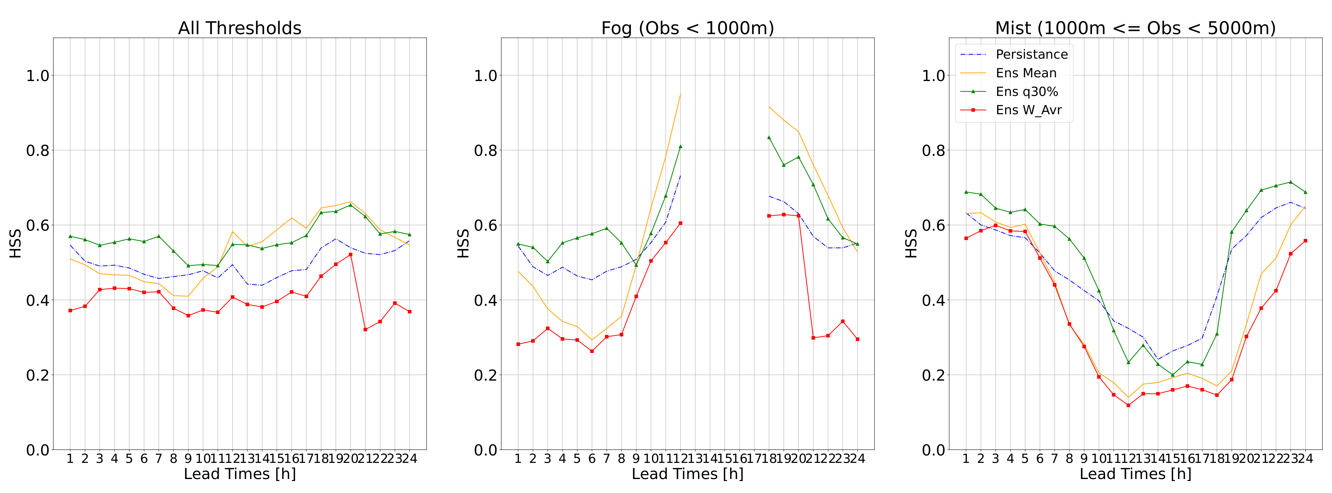
Here, AnEn performance is investigated for a lead time of 24 h based on the HSS metric (Figure 8). The HSS is computed and averaged over all locations for all visibility thresholds (from 200 m to 6000 m by a step of 200 m) over the testing period (2019). HSS values are averaged for each lead time for all studied thresholds and are plotted in Figure 8. A special focus is placed on fog (threshold equal to 1000 m) and mist events (thresholds between 1000 m and 5000 m). From Figure 8, it can be seen clearly that for all the thresholds and also for LVC conditions, AnEn quantile 30 outperforms persistence with an averaged HSS of around 0.6 compared with 0.5 for persistence (all visibility thresholds). It should be noted that HSS for fog event prediction improved during the daytime and reached 0.8, while it deteriorated for mist event prediction and reached 0.2. For the other AnEn configurations, it is found that the AnEn mean shows a similar HSS performance to AnEn quantile 30 during the daytime and early night for all visibility thresholds and fog event forecasting, while it is outperformed for mist event cases. The AnEn weighted mean configuration is found to be the worst configuration for all cases.

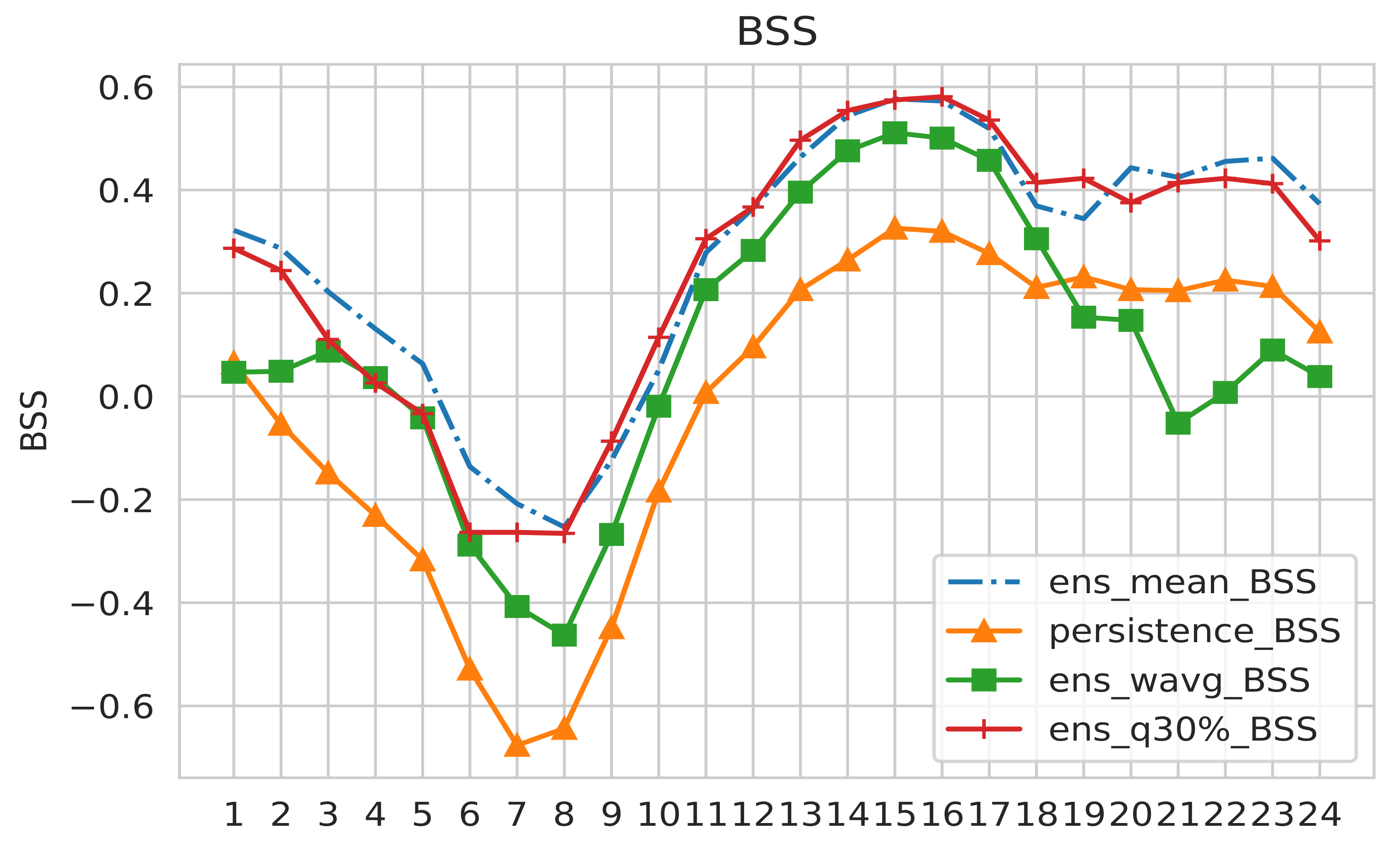
Figure 9 displays the BSS (see Appendix A) at each lead time for LVC events where the visibility is below 5000 m for all AnEn configurations (mean, weighted average, quantile 30%) with persistence as the benchmark. The BSS is used to assess the relative skill of the probabilistic forecast over that of climatology, in terms of predicting whether or not an event occurred. It is important to mention here that 1 is a perfect score of BSS associated with a null Brier Skill Score (the average square error of a probability forecast). When BSS is approaching zero, it reflects no improvement in the AnEn forecasting system over the reference (climatology). From Figure 9, it can be seen that the AnEn mean and AnEn quantile 30% show the best BSS among all AnEn configurations and persistence. However it is important to mention that the best BSS scores are only restricted to lead times after 10 h or earlier than 4 h. Indeed, BSS reached values above 0.4 after 12 h. On the other hand, climatology (as the reference) outperforms the AnEn forecasting system during the morning. It should be noted that this skill score is very sensitive to the rarity of the studied event and requires a larger number of samples to stabilize it.

4.3.4. Performance as a Function of LVC Thresholds (BSS and HSS)

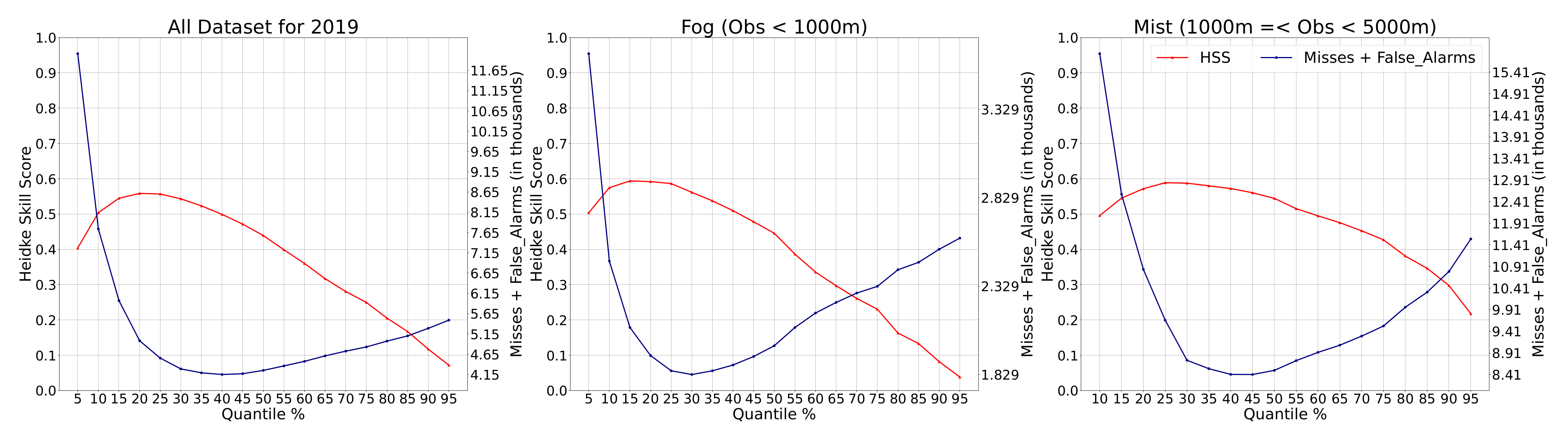
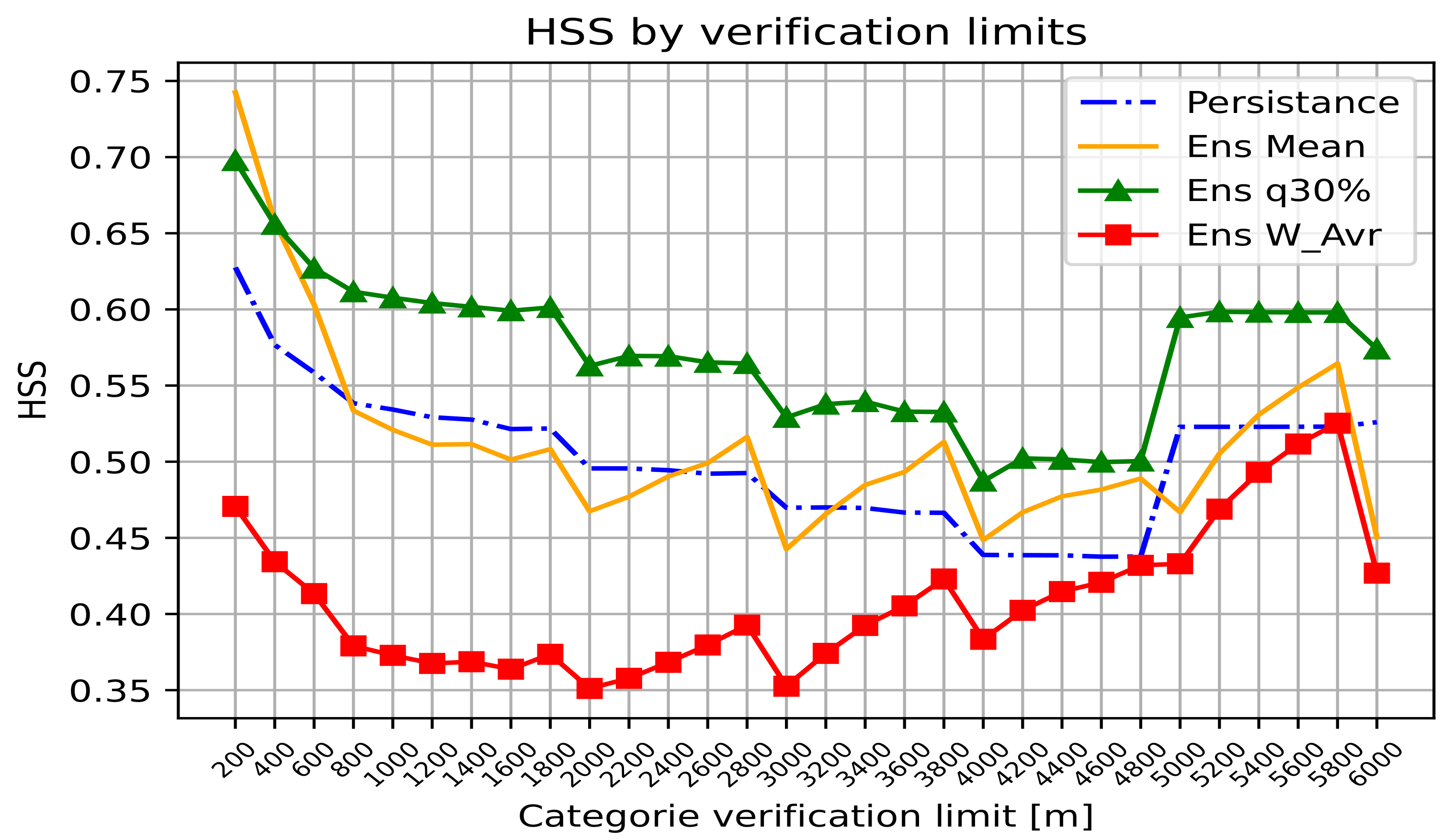
We define LVC thresholds from 200 m to 6000 m by a step of 200 m. Then, HSS is computed for the three AnEn configurations (AnEn mean, AnEn weighted mean, and AnEn quantile 30%) and for each visibility limit. The averaged HSS values for all locations as a function of LVC thresholds are plotted in Figure 10. On average, AnEn quantile 30% (green) shows a better HSS than persistence (dashed line) for all LVC thresholds, while the AnEn weighted mean shows the worst performance. The best HSS scores (above 0.6) are found for thresholds lower than 1800 m and above 4800 m. For the limits between 2000 and 4600 m, the AnEn quantile 30% shows a constant HSS between 0.5 and 0.55. From Figure 10, one can notice that AnEn mean (orange) and AnEn weighted average (red) performances improve with higher visibility thresholds. This reveals the highest sensitivity of the ensemble mean as a verification metric for rare events.

In Figure 11, the BSS is averaged over all lead times for each LVC threshold. In this study, the thresholds vary from 200 m to 6000 m by a step of 200 m. This figure confirms that AnEn quantile 30% yields the best AnEn configuration, which outperforms all other configurations and also persistence. It displays a quite good BSS for LVC events, particularly where the visibility threshold is lower than 1000 m (BSS around 0.4).

5. Discussion

Predicting rare weather events is always a challenging process. Despite all of the advances in NWP deterministic models, these models show several uncertainties, occasioned by several error sources related to model formulation [36], initial state [37], physical parameterization [38], and lateral boundary conditions [39]. In the face of these limitations, ensemble prediction takes advantage of all of these sources of uncertainty to construct multiple forecasts, and thus provides a reliable alternative to single out a deterministic scenario. However, even in the usage of ensemble forecasting, several limitations and challenges are encountered. Indeed, rare event forecasting remains arduous due to three elements: (a) the definition of a rare event itself and the setting of its thresholds, (b) rare event sampling, and (c) the sensitivity of the outcomes to user decisions or verification interpretability.

Many studies provide probabilistic forecasting frameworks for weather extreme events using ensemble forecasting. The application of such an approach covers flood forecasting [40,41], ozone prediction [42,43], heat waves [44], and severe weather [45,46]. From the previous research works, ensemble forecasting potential in assessing rare events is highly encouraged. Nevertheless, two main difficulties are raised: first, the definition of a rare event [47,48], and second, the high computational cost of the classical ensemble approaches dealing with extreme events and their verification.

The analog ensemble forecasting method answers the second issue and provides an economic alternative [49]. Indeed, AnEn is a good technique to reduce the bias of low-visibility/fog prediction if some factors are carefully controlled, such as the selection of the best historic runs and weights, the data sample size of rare low-visibility events, training time length, etc. Moreover, in dealing with rare events, this method has been widely applied. The authors in [50] present a new approach in correcting analog ensemble probabilistic forecasts. The proposed method shows great improvement in predicting extreme wind events. The latter raises the need for tuning the rare event threshold for other variables or datasets. This issue was assessed in our work by selecting the best AnEn quantile depending on the visibility thresholds.

The lack of good-quality analogs enhances conditional biases from the AnEn when predicting rare events, resulting in a left tail of forecast PDFs [51]. Indeed, good analog quality is assured by the quality of the predictors, which must reveal a physical link to the target variable. On the other hand, the quality of the analogs depends also on the length of the training period [52,53], which in our case covers 3 years.

In the same context, selecting the most relevant predictors is vital to any efficient AnEn application. For visibility forecasting, including $N_d$ in the set of predictors can be of high importance. Hence, using more complex parametrizations of visibility [1,12,54,55,56] is more needed than ever.

Few works have applied analog ensembles to predict horizontal visibility. For instance, the analog ensemble method shows promoting results, as demonstrated in reference [13], where the proposed method shows an HSS of 0.56, using a fuzzy-logic-based similarity metric. In this study, the analog ensemble method based on quantile 30% shows a good performance with a HSS of about 0.65 for all LVC thresholds. This points out the high proportion of correct forecasts out of those relative to random chance.

The analysis of the results shows that the HSS score displays a high sensitivity to visibility thresholds, since the best scores are found for thresholds below 1800 m or above 4800 m. These findings are in line with the findings in [26], where the authors proposed a new hybrid analog-based method to predict horizontal visibility and used the main standard meteorological variables from METARs. The authors in [26] suggested the inclusion of new parameters in visibility AnEn forecasting. This was assessed in this work since the six major weather variables are used as predictors (T2m, RH2m, WS10m, WD10m, SURFP, and MSLP). In addition, two highly influential parameters for low-visibility events were added as well (liquid water content at 2 m and 5 m).

Setting a rare event threshold shrinks data samples, hence making the finding of a rare event harder. One of the major challenges in the ensemble forecast verification process is the limited proportion of available data which in some cases may not include extreme events [57]. This issue may lead to the misleading interpretation of verification scores since the system of prediction reveals high hit scores that refer mainly to high numbers of non-event occurrences. In our work, we defined a low-visibility rare event as a horizontal visibility lower than the selected thresholds. A range of thresholds from 200 m to 6000 m by 200 m was explored for verification. In addition, there was a focus on fog and mist conventional thresholds of 1000 m and 5000 m, respectively, for the whole year of the test (2019). As a result, it was found that AnEn shows an averaged HSS of about 0.65. Furthermore, we revealed the higher sensitivity of the AnEn performances to statistical metrics such as mean, weighted average, and best quantile.

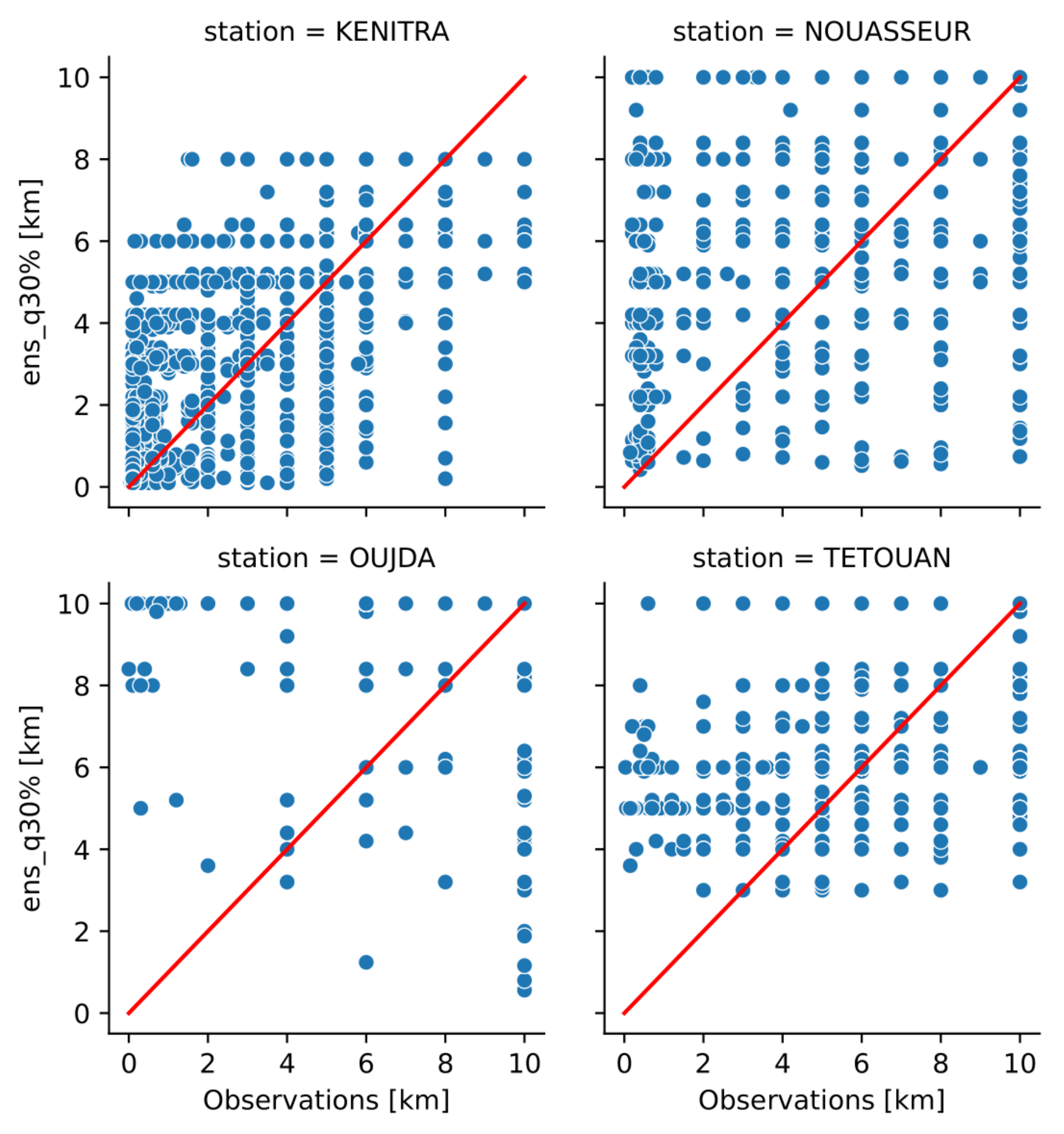
To illustrate the dependence of the AnEn method’s performance on geographic position, scatter plots of predicted visibility versus the observed one are shown in Figure 12: Kenitra (a coastal station in the western part), Nouasseur (an inland station in the western part), Oujda (an inland station in the eastern part), and Tetouan (a coastal station in the northern part). This figure points out that for the foggy stations (Kenitra and Nouasseur), AnEn quantile 30% is able to capture some LVC events, while for the other stations, the developed forecasting system has a weaker performance for fog and mist event prediction.

6. Conclusions and Perspectives

In this study, an ensemble analog-based system is implemented to predict low-visibility conditions over 15 airports of Morocco. The continuous and probabilistic verifications were performed over one year based on three outputs (ensemble mean, ensemble weighted mean, and ensemble best quantile). The verification process was carried out for three use cases: (a) the whole dataset, (b) fog events, and (c) mist events.

When considering spread–skill diagrams and rank histograms, AnEn was found to be under-dispersive for all lead times and draws a positive bias for fog and mist events, while it was quite statistically consistent for the whole dataset. For the whole testing dataset, AnEn mean and weighted average had the lowest bias, whereas AnEn quantile 30% was the best for fog and mist cases. Furthermore, AnEn is reliable for the most propitious low-visibility lead times (night and early morning), while it underestimated visibility for day lead times.

Globally, AnEn RMS errors were geographically and lead-time-dependent and became higher for low-visibility cases. However, AnEn had the lowest errors compared with persistence for all configurations, associated with a high correlation over the whole dataset and weak one for fog and mist events. In comparison with the AnEn mean and AnEn weighted mean configurations, the CRMSE of AnEn quantile 30% deteriorated when removing bias from forecasts and observations for fog and mist cases. Analysis of the decomposition of RMSE into systematic and random errors points out that errors are provided mainly by random chance for the whole spectrum of visibilities over the testing period, while they are associated with systematic errors for specific low-visibility cases.

When converting all AnEn continuous outcomes to binary forecasts for a set of thresholds from 200 m to 6000 m by a step of 200 m, performances in terms of HSS are highly dependent on the chosen threshold. Hence, the best HSS was found for thresholds lower than 1000 m or greater than 4900 m, which matches fog and mist thresholds. The best HSS scores were exhibited by AnEn quantile 30%, especially for night and early-morning lead times. For fog events, AnEn 30% quantile had the best HSS for lead times below 6 h, whereas for lead times above 18 h AnEn mean was superior. During mist events, the best quantile of AnEn outperformed persistence during night and early-morning lead times. For day lead times, their performances were quite the same.

In terms of probabilistic verification, AnEn 30% quantile shows the best performance among all AnEn configurations and surpasses persistence. However, for continuous verification (Bias, CC, and CRMSE), the best AnEn performances are generally seen during night and early-morning lead times. However, when focusing on specific low-visibility conditions such as fog or mist, AnEn performances become weaker. When combining bias, CC, and CRMSE results, the RMS error for all visibilities over the whole year of 2019 is mainly produced by random errors, since correlation for the whole dataset is above 0.6 and the magnitude of CRMSE is greater than that of bias. However, for low-visibility conditions (fog and mist), we found lower CC values (below 0.5) associated with errors that are mainly systematic (the magnitude of CRMSE is lower than that of bias).

In this study, the selection of analogs considered only historical data for each grid point in the study domain closest to the observation site. Thus, to enhance the chances of finding the best analogs, one could extend the search space by integrating neighboring grid points. A path of amelioration would be to use some calibration methods for rare events [50] to overcome the disproportionality of such events in the sampling. Another method of improvement is to use new sampling methods, such as subset simulation algorithms [58], which enhance the speed of calculating rare event probabilities.