Relations between Urban Entropies, Geographical Configurations, Habitability and Sustainability

Abstract

This study examines the consequences of human activity on the atmospheric boundary layer considering (i) atmospheric pollution, (ii) urban micrometeorology, (iii) three geographic morphologies (mountain, basin and coast) and (iv) surface change of roughness due to buildings. Qualitative relationships are established between the four issues mentioned using measurements from different periods, urban meteorology and pollutants, in the boundary layer of the three geographic morphologies, all with large urban settlements. The measurements per hour and at ground level correspond to the variables: temperature, magnitude of wind speed, relative humidity and concentration of anthropogenic pollutants (PM₁₀, PM_2.5 and CO). The measurements form time series, demonstrating their chaoticity through the parameters: Lyapunov coefficient, correlation dimension, Hurst coefficient, Lempel–Ziv complexity, information loss, fractal dimension and correlation entropy. The results, according to each parameter, allow us to characterize the effect of human activity on geographical morphologies and its meteorology, showing a lower impact on mountain and coastal areas. Calculating, for each geographical configuration, the quotient between the total correlation entropy of the meteorological variables and that of the pollutants, the basin entropy is less than one, which shows, for the study period, the entropic domain of atmospheric pollutants unlike mountain and coast.

1. Introduction

The consequences of human activity on the atmospheric boundary layer have been discussed in the literature [1,2]. For the studies that consider air pollution, urban micrometeorology and the change in surface roughness produced by cities, this work incorporates the effect of geographic morphologies [1,2,3]. To determine relationships between the indicated topics, chaos theory and its chaotic parameters, such as entropy, Hurst coefficient and loss of information, are used, which are calculated from time series of measurements of meteorological variables and atmospheric pollutants. The analysis reveals the presence of irreversible processes and, in addition, allows comparisons to be made between “urbanized” morphologies, qualitatively exposing the contribution of cities to climate change and global warming. Similar consequences are reviewed in other countries to check the proposal. The problem exceeds borders, but extreme solutions such as the intervention by climatic geoengineering in global warming is an option with a high degree of uncertainty in its consequences [2,3] due to the variety of factors, on the micro scale, that originate. The results show that the current way of developing cities gives sustainability to climate change and global warming.

1.1. Urban Microclimates

A microclimate is an environmental system that contains atmospheric patterns and processes that are defined in a reduced environment. Its components are topography, temperature, altitude–latitude, light and vegetation cover, in which human activities take place (urban architecture, industries, economic processes, etc.) that can affect atmospheric variables. To mitigate extreme weather conditions, a series of engineering machines (air conditioning in hot periods, heating in cold times, air purifiers, etc.) have been implemented, which have made it possible to soften extreme conditions (of a place, generally urban), and which end up transforming the climate on a local scale [4].

In addition to natural microclimates, there are also artificial microclimates, which originate, especially, in urban areas due to large emissions of heat and greenhouse gases [5]. The influences of urban structures and their materials can determine the behavior of the climate in public spaces, considering the usual elements in construction and their albedos (a) and emissivity (e) [6], respectively: asphalt, fresh–old (a = 0.05–0.2, e = 0.95); wet or dry soil (a = 0.05–0.4, e = 0.98–0.90); walls–concrete (a = 0.10–0.35, e = 0.94); walls–stone (a = 0.20–0.40, e = 0.85–0.95); floor tiles (a = 0.100.35); grass (a = 0.16–0.26, e = 0.90–0.95); dry clay (a = 0.23); corrugated steel (a = 0.10–0.16); bright galvanized steel (a = 0.35, e = 0.13).

There is a relationship between morphological descriptors, which correlate the shape of the urban space, and its climatic behavior [7,8]. In the urban space, we find the urban canyon [6] and the infrastructure that contains it, relative height, width of the street and the spatial continuity factor of the street [9,10,11]. Similarly, vehicular mobility is another important factor to consider due to its high impact on the behavior of the wind at pedestrian level.

1.2. Geomorphology

It studies the shapes of the earth’s surface in order to describe and understand its genesis and its current behavior [12]. This article focuses on cities that may be located in a basin (a basin is a depression in the earth’s surface, a valley surrounded by heights) with a confined wind regime. It also focuses on those located in coastal areas, which are commonly defined as the zones of interaction or transition between land and sea, including large continental lakes. Coastal zones are diverse in dynamics, function and form and are difficult to define according to strict spatial criteria. Finally, it explores human settlements in high mountain areas with good ventilation. Figure 1, Figure 2 and Figure 3 show the types of geography profiles present in Chile:

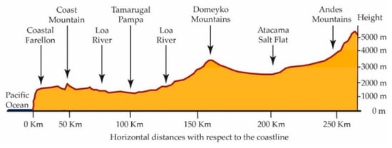
Figure 1. Chile’s Great North Topographic Profile 22° and 23° South Latitude.

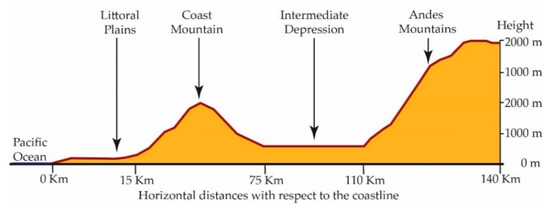
Figure 2. Topographic profile central zone of Chile 33° South Latitude.

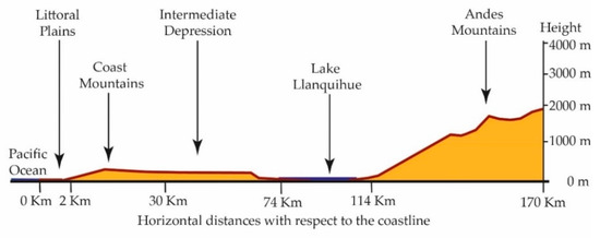
Figure 3. Topographic profile 41° Latitude South of Chile.

1.3. Geography and Wind Regimes

If we consider the natural dynamics of Valley–Mountain breezes, solar radiation arrives nonuniformly on the slopes of mountains and valleys. In addition, the radiation changes its angle of incidence according to the time of day due to the apparent movement of the sun. The thermal flow of air generated is restricted by the centers of high and low pressure induced by the differences in daily temperatures produced between the valley and the mountains [13]. On the other hand, there is an unequal thermal behavior of water and land [14].

1.4. Local Winds

Local winds, similar to other types of winds, present a displacement of air from high-pressure areas to low-pressure areas, establishing dominant winds [15] in a more or less extensive area. These types of winds are: sea and land breezes; valley breezes; mountain breezes. Katabatic winds are those that descend from the heights to the bottom of the valleys, produced by the sliding at ground level of cold and dense air from the highest reliefs [13]. The anabatic wind is one that rises from the lowest to the highest areas as the sun heats the relief (Figure 4).

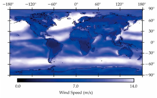
Figure 4. Annual wind speed at 10 m for airport-like terrain. July 1983–June 1993. (Public archive, NASA/SSE, 13 September 2004). The figure shows the zone of equatorial calms and, to the south, the belt of strong subantarctic katabatic winds.

1.5. Contaminants in This Study

Atmospheric pollution consists of the release of large amounts of harmful elements whose concentration levels affect all forms of life and their habitat. Atmospheric aerosols (or particulate matter, PM (measured in µm, 1 µ =${10}^{-6}$)) are made up of solid or liquid particles [16]. These can be classified according to their size. PM₁₀ is made up of particles with a diameter equal to or less than 10 µm, while PM_2.5 are those with a diameter equal to or less than 2.5 µm. Since PM_2.5 is contained in PM₁₀, we can say that PM_2.5 is the fine fraction of PM₁₀. Particles with a diameter between 2.5 µm and 10 µm are considered to constitute the coarse fraction of PM₁₀. However, there is also an ultrafine and even nanometric fraction. Currently, there are many studies that show the damage that pollution causes to human health [17,18,19,20,21,22,23,24,25].

Carbon monoxide (CO) is a dangerous gas that you cannot smell, taste or see. It occurs when carbon-based fuels such as kerosene, gasoline, natural gas, propane, coal or wood are burned without enough oxygen, and can cause long-term vision problems when inhaled. Table 1 gives a summary of these effects:

Table 1. Effects of CO on people according to exposure time.

Concentration in the Air	Effects
55 mg/m3 (50 ppm)	TLV–TWA * Normal working day of 8 h or one week 40 h without showing adverse effects.
0.01%	Exposure of several hours without effect.
0.04–0.05%	One hour exposure without effect.
0.06–0.07%	Appreciable effects at the time.
0.12–0.15%	Dangerous effects after one hour.
165 mg/m3 (1200 ppm)	Immediate danger to life and health (IDLH).
0.4%	Fatal after one hour.

* TLV-TWA is the concentration corresponding to a normal 8 h day or a 40 h week of occupational exposure without presenting harmful effects.

1.6. Meteorological Variables

This work uses the hourly records of the relative humidity (RH), the temperature (T) and the magnitude of the wind speed (WS) that, in a first approximation, allow us to describe the atmospheric dynamics [9]. Atmospheric pressure is one of the less notable weather variables, since its daily variations on the surface are not perceptible, unlike the temperature, precipitation, relative humidity or wind. However, due to its relationship with other meteorological variables, variations in atmospheric pressure are a relevant factor in weather forecasting [26].

The hypothesis of this work is that in geographic morphologies where urban meteorology dominates over pollutants (measured in this research), the atmospheric layer adjacent to the ground is more ventilated, while in the sectors with boxed valleys (basin), contaminants dominate. This phenomenon is analyzed through chaos theory and the calculation of correlation entropy (or Kolmogorov). Although the ventilation factor is critical in relation to the selected contaminants, chaotic studies are favorable when there is connectivity between the variables, characteristic of irreversible processes and complex systems. Ventilation is explained in Figure 5 and Figure 6:

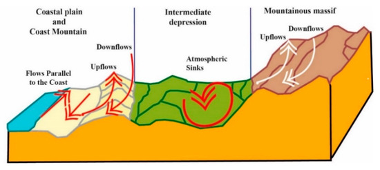
Figure 5. Human settlements according to geographic profile and wind dynamics.

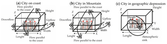
Figure 6. Atmosphere cell model for wind flow dynamics.

2. Theoretical Bases

2.1. Kolmogorov Entropy and Its Relation to Information Loss

Following Farmer [27], the basic difference between chaotic and predictable behavior is that chaotic trajectories constantly produce new information, while predictable trajectories do not [27,28]. Metric entropy presents this difference more precisely, providing a good definition of “chaos” and providing a quantifiable method of describing “how chaotic” a dynamical system is. The Kolmogorov entropy [29,30], S_K, is defined as the average information loss [31,32] when “l” (cell side in information units) and τ (time) become infinitesimal:

$${\mathrm{S}}_{\mathrm{K}}=-\underset{\mathsf{\tau }\to 0}{\lim }\underset{\mathrm{l}\to 0}{\lim }\underset{\mathrm{n}\to \infty }{\lim }\frac{\mathrm{l}}{\mathrm{n}\mathsf{\tau }}{\displaystyle \sum }_{0\dots .\mathrm{n}}{\mathrm{P}}_{0\dots .\mathrm{n}}\log {\mathrm{P}}_{0\dots ..\mathrm{n}}$$

(1)

The unit of measure is in bits of information/second and bits per iteration for a discrete system [33,34]. To calculate the limit of Equation (1), the order of priority is as follows: (i) n→$\infty$ (ii) l→0, thus eliminating the dependence on the chosen partition. In the limit (Equation (1)), n is the number of cells or partitions. The calculation, (iii) τ→$0$, is applied in continuous systems. Upon determining the Kolmogorov entropy difference ΔS_K = S_Kn+1 − S_Kn between one cell and another, the additional information required to know in which cell (i_n+1) the system will be in the future is obtained. Therefore, the difference measures the loss of system information over time.

By calculating S_K, it follows: 0 < S_K < $\infty$, presence of chaotic behavior; S_K = 0, no information is lost and the system is regular and predictable; S_K = $\infty$, the system is completely random and predictions are impossible. It is possible to apply this procedure to find the amount of information required to predict the future behavior of two interacting systems: in this case, urban meteorology pollutants. In this way, it is possible to calculate the rate at which the system loses (or outdates) information over time. From this information, the horizon of maximum predictability of the system can be obtained, which is the frontier from which it is not possible to make predictions or deploy new descriptive frameworks [29].

2.2. Information Loss

Information loss can be calculated according to:

$$<\Delta \mathrm{I}> = <{\mathrm{I}}_{\mathrm{NEW}}-{\mathrm{I}}_{\mathrm{OLD}}\ge \frac{-\mathsf{\lambda }\left({\mathrm{i}}_0\left(\mathrm{t}\right)\right)}{\log 2}$$

(2)

λ corresponds to the Lyapunov exponent, <ΔI> in [bits/h], this refers to the loss of information. From the measured data, two types of <ΔI> could be obtained: one for the contributions of each P (pollutants: PM₁₀, PM_2.5 and CO) and another for the contributions of each MV (meteorological variables: T, WV, RH).

3. Materials and Methods

3.1. Study Area

A map shows the monitoring stations (black asterisk *) of Chile, Mexico City and Quito in Ecuador used in this study (Figure 7). Table 2 indicates the characteristics of the climate, geography, type of pollutants and meteorology:

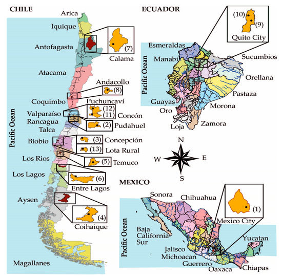
Figure 7. Study countries and locations.

Table 2. The measurement locations, shown in Figure 7, and their specifications. Some with locality code and others not informed (NI), meters above sea level (masl), geography, pollutants and meteorology (Wind, average annual temperature (T) and average annual relative humidity (HR%)) [35,36,37].

Station Name	Geography	Climate	Pollution	Wind	T (°C)	RH (%)
1. Pudahuel, EMO, masl: 469 (m)	Located at the bottom of the basin	Cold, dry winters, hot, dry summers.	Presence in descending order PM10, PM2.5, CO, SO2, NO2, O3	South–East day East–South night	15.3	57.7
2. Kingston College, NI, masl: 12 (m)	River edge plain	Cool, wet summers and cold, wet winters	Presence in descending order PM2.5, CO, PM10, SO2, NO2, O3	North West–South East day East–North West night	13.3	75.2
3. Coyhaique, NI, masl: 310 (m)	Inland valley plain	Cold and wet winters and summers	Presence in descending order PM2.5, PM10	North West–East day East–West South night	4.8	82
4. Las Encinas, NI, masl: 360 (m)	Inland valley plain	Cool, wet summers and cold, wet winters	Presence in descending order PM10, PM2.5, CO, SO2, NO2, O3	West–North East day East–West night	11.4	64.5
5. Entre Lagos, NI, masl: 39 (m)	Undulating sectors of the intermediate depression	Cool, wet summers and cold, wet winters	Presence in descending order PM2.5, CO, PM10, SO2, NO2	East–West day West–East night	14	83
6. Mexico City, BJU, masl: 2250 (m)	Valley bottom plain	Warm and dry in summer and cool and wet in winter	Presence in descending order PM10, PM2.5, CO	North–East day East–West night	16	58.8
7. Center Station, NI, masl: 2400 (m)	Valley bottom plain	Cool, dry winters and mild, dry summers	Presence in descending order PM10, PM2.5, CO, SO2, NO2, O3	West–North East day East–West night	17.2	28.8
8. Andacollo, NI, masl: 1017 (m)	Coastal mountain range plain	Cool, dry winters and hot, dry summers	PM10	North–South East day East–West night	21	60
9. Tumbaco, NI, masl: 2331 (m)	Cordilleran plain	Cool and wet in winter and warm and wet in summer	Presence in descending order PM10, SO2, O3	North West–South East day Sout East–North West night	16	86
10. Carapungo, NI, masl: 2851 (m)	Cordilleran valley bottom plain	Cool and wet in winter and warm and wet in summer	Presence in descending order PM10, PM2.5, CO, SO2, NOx, O3	North West–East day East–West night	11.3	86.1
11. Concon, NI, masl: 2 (m)	Sector between coastal plain and coastal mountain range	Hot, dry summers, cold, wet winters	Presence in descending order PM10, PM2.5, CO, SO2, NO2, O3	West–East day East–West night	15	69.5
12. Loncura, NI, masl: 3 (m)	Hill near the coast	Hot, dry summers, cold, wet winters	Presence in descending order PM10, PM2.5, CO, SO2, NO2, O3	West–East day East–West night	15.1	71.5
13. Lota Rural Station, NI, masl: 16 (m)	Creek and coastal hill	Cool, wet summers and cold, wet winters	Presence in descending order PM2.5, CO, PM10, SO2, NO2, O3	West–East day East–West night	12.7	73.8

3.2. The Data

The time series of hourly concentrations of pollutants (PM₁₀, PM_2.5 and CO) and meteorological variables (T, HR and VV) of Chile were compiled from the public network MACAM III, belonging to SINCA (National Information System of Quality of the Air), dependent on the Chilean Ministry of the Environment (MMA, 2019), with a total of 10 locations with morphological characteristics of basin (5), mountain (2) and coast (3). The methodology is tested in other countries: Mexico, Mexico City (basin morphology) and in Ecuador, in the mountain cities of Tumbaco and Carapungo. In these countries, the databases of their local environmental information acquisition systems were used. Table 3 presents the measurement instruments used in the different locations of the study:

Table 3. Measurement instruments in the 13 locations studied. NI: Without information of the locality code. The capital letters in each box indicate the type of measurement instrument used in the different locations of the study (the meaning of each capital letter with the details of each instrument appears at the end in Abbreviations before the References).

Station Name	Location	PM10	PM2.5	CO	T	RH	WV	Owner
1. Pudahuel, EMO, masl: 469 (m)	33°27′06.2″ S 70°40′07.8″ W	A	A	B	C	C	D	SINCA
2. Kingston College, NI, masl: 12 (m)	36°47′4.74″ S 73°3′7.42″ O	E	E	F	G	G	H	SINCA
3. Coyhaique, NI, masl: 310 (m)	45°34′44.57″ S 72°2′59.88″ O	A	A	I	J	J	K	SINCA
4. Las Encinas, NI, masl: 360 (m)	38°44′55.38″ S 72°37′14.54″ O	A	A	I	L	L	L	SINCA
5. Entre Lagos, NI, masl: 39 (m)	40°41′2.36″ S 72°35′47.25″ O	E	E	F	F	F	F	SINCA
6. Mexico City, BJU, Mexico masl: 2250 (m)	19°22′12.00″ N 99°9′36.00″ O	F	F	F	F	F	F	SINAICA
7. Center Station, NI, masl: 2400 (m)	22°27′42.55″ S 68°55′41.45″ O	N	N	M	O	P	Q	SINCA
8. Andacollo, NI, masl: 1017 (m)	30°13′39.94″ S 71°5′10.09″ O	A	$-$	$-$	R	R	S	SINCA
9. Tumbaco, NI, Ecuador masl: 2331 (m)	0°12′36′’ S 78°24′00′’ W	T	T	U	V	V	D	SUIA
10. Carapungo, NI, Ecuador masl: 2851 (m)	0°5′54′’ S 78°26′50′’ W	T	W	B	V	V	D	SUIA
11. Concon, NI, masl: 2 (m)	32°55′29.12″ S 71°30′55.73″ O	N	N	X	O	Y	Z	SINCA
12. Loncura, NI, masl: 3 (m)	32°47′41.69″ S 71°29′47.11″ O	E	E	AA	P	Y	H	SINCA
13. Lota Rural Station, NI, masl: 16 (m)	37°6′0.70″ S 73°9′7.87″ O	AB	AB	AC	G	G	AD	SINCA

It is common to find missing data in this type of series, which may be due to different factors [38,39,40]. Missing data were filled using the Kriging technique [9,41,42]. In particular, the applied technique is the spatiotemporal geostatistical method, which provides a probabilistic framework for data analysis and prediction, based on the joint spatial and temporal dependence between observations [43].

3.3. Mathematical Method Used in the Analysis of Nonlinear Time Series

For the analysis of time series and some chaotic parameters, nonlinear tools [44,45] were used, such as the Chaos Data Analyzer software [46,47]. The reason is that, in the phenomena associated with this type of data, small perturbations generate large effects on future values [48]. This is the essence of nonlinearity (dependence sensitive to initial conditions or “butterfly” effect) and even more chaos in its evolution [49,50,51].

For the study of nonlinear time series, the procedure indicated in [9] is followed. Taken’s procedure [52] can be applied to τ, which gives the time delay (lagging time) and m (or dc) which gives the embedding dimension. In the temporal delay, the average mutual information is applied [53], and for the embedding dimension, false nearest neighbors are used [51,54]. Essential parameters (or metrical quantities) in nonlinear time series analysis are: time lagging, τ, the Lyapunov’s exponent, λ [55], the correlation dimension (correlation function), D_C [47], the Kolmogorov entropy, S_K, the Hurst coefficient, H (0 < H < 1) [47,56] and the correlation entropy, K₂. To define the Lyapunov’s exponent, two arbitrary samples from the series xi and xj can be used. For that purpose, first let d₀ = ‖x_i − x_j‖ be the initial distance between two arbitrary samples of the series x_i and x_j. Second, assuming that the distance d_n = ‖x_(i+n) $-$ x_(j+n)‖ between two samples at position n grows exponentially with n, then the Lyapunov’s exponent, λ, is defined [16]:

$$\mathsf{\lambda }=\frac{1}{\mathrm{n}}\ln \frac{{\mathrm{d}}_{\mathrm{n}}}{{\mathrm{d}}_0}$$

(3)

where n is the iteration number (number of points in the time series). This is equivalent to considering two nearest neighbor points in an orbit and calculating the exponent for a large value of n. If, after carrying out n iterations, the neighboring points separate, it is a sign of possible chaos in the system, since the saturation becomes evident. If λ > 0 for the maximum Lyapunov’s value, it is an indication of chaos [44,47]. For a given time series, the result of adding all the positive Lyapunov’s exponents allows us to calculate its entropy, S_K. The average predictability time is given by T_P = 1/S_K [51]. The stability conditions in the numerical calculation of the Lyapunov exponent require a large amount of data (at least 5000 available data) [57]. The correlation entropy, K₂ [47,58,59] is defined as:

$${\mathrm{K}}_2=\underset{\mathrm{m}\to \infty }{\lim }\underset{\mathrm{r}\to 0}{\lim }\underset{\mathrm{n}\to \infty }{\lim }\log \frac{\mathrm{C}\left(\mathrm{m},\mathrm{r}\right)}{\mathrm{C}\left(\mathrm{m}+1,\mathrm{r}\right)}$$

(4)

where m is the embedding dimension and r is the radius of the circle or sphere. Depending on the value of K₂, it is possible to characterize the data of the time series according to: K₂ = 0, regular data; K₂ > 0 chaotic data; K₂ = ∞, random data. This criterion is applied to experimental time series of pollutants and meteorological variables.

C (m, r) (Equation (5)) is the correlation sum of the reconstructed path of a time series according to a given embedding dimension, m. Grassberger and Procacia [56] provide a method to estimate K₂ in time series of experimental data. In this study, the Kolmogorov entropy, S_K, was determined for the series of pollutants and the meteorological variables. C (m, r) allows estimation of the correlation dimension [47], defined as:

$$\mathrm{C}\left(\mathrm{r}\right)=\frac{2}{\mathrm{n}\left(\mathrm{n}-1\right)}{\displaystyle \sum }_{\mathrm{j}=1}^{\mathrm{n}}{\displaystyle \sum }_{\mathrm{i}=\mathrm{j}+1}^{\mathrm{n}}\mathrm{H}\left(\mathrm{r}-{\mathrm{r}}_{\mathrm{ij}}\right)=\underset{\mathrm{n}\to \infty }{\lim }\frac{2}{\mathrm{n}\left(\mathrm{n}-1\right)}{\displaystyle \sum }_{\mathrm{i}\ne \mathrm{j}}^{\mathrm{n}}\mathrm{H}\left(\mathrm{r}-\Vert {\mathrm{x}}_{\mathrm{i}}-{\mathrm{x}}_{\mathrm{j}}\Vert \right)\to \mathrm{C}\left(\mathrm{m},\mathrm{r}\right)$$

(5)

where ${\mathrm{r}}_{\mathrm{ij}}=\sqrt{{\displaystyle \sum }_{\mathrm{k}=0}^{\mathrm{m}-1}{\left({\mathrm{x}}_{\mathrm{i}-\mathrm{k}}-{\mathrm{x}}_{\mathrm{j}-\mathrm{k}}\right)}^2}$ (the sum depends of m (embedding)), C(r) is the function of the correlation, and it can be interpreted as the number of points inside all the circles of radius r normalized to one, when r is big enough that it includes all the points without double counting. N is the number of data, H is the Heaviside function or (step function). ‖…‖ shows the norm or distance between two vectors, where the Euclidean one is the most used one, since it offers stronger results even during noise, and r is a real number that must be chosen carefully, since small r values make C(r) senseless, and for bigger r values, C(r) does not provide valuable information.

Equation (5) can also be written as follows:

$$\mathrm{C}\left(\mathrm{r}\right)=\underset{\mathrm{n}\to 0}{\lim }\frac{1}{{\mathrm{n}}^2}\left[\mathrm{number} \mathrm{of} \mathrm{pairs} \left({\mathrm{x}}_{\mathrm{i}},{\mathrm{x}}_{\mathrm{j}}\right) \mathrm{such} \mathrm{that} \left|{\mathrm{x}}_{\mathrm{i}}-{\mathrm{x}}_{\mathrm{j}}\right|<\mathrm{r}\right]$$

(6)

C(r) is calculated as 0$\le$ r $\to$ largest possible number of $\Vert {\mathrm{x}}_{\mathrm{i}}-{\mathrm{x}}_{\mathrm{j}}\Vert$. If the values of r are small enough and n large enough, C(r) follows the power law:

$$\mathrm{C}\left(\mathrm{r}\right)~{\mathrm{r}}^{{\mathrm{D}}_{\mathrm{C}}}$$

(7)

If a logarithm is applied to Equation (7), the value of D_C is determined from a graph log C(r) vs. Log r. Three conditions emerge for D_C, according to the graph: (i) if it does not saturate at any value as m increases, the process is random (or stochastic). (ii) If it saturates at some value, the time series is deterministic [60]. Table 4 of this study, from the chaotic analysis of the time series (6), shows the values for which there was saturation. (iii) If the correlation dimension is greater than 5, it means essentially random data, a condition that is not present in this study.

Table 4. Table presents the summary of the calculations, where h is hour and masl is meters above sea level.

Basin	Variables Each 17,520 h	λ (Bits)	Dc	Sk (Bits/h)	H	LZ	<ΔI>
	CO	0.017 ± 0.006	2.937 ± 0.115	0.459	0.933	0.014	−0.056
(a) Pudahuel	PM10	0.593 ± 0.030	3.531 ± 1.665	0.246	0.942	0.178	−1.970
	PM2.5	0.260 ± 0.026	1.231 ± 0.309	0.326	0.919	0.309	−0.864
					0.931		−0.963
(2018−2019, 584 masl)	T	0.261 ± 0.016	2.551 ± 0.069	0.289	0.917	0.238	−0.867
	WS	0.960 ± 0.018	4.029 ± 0.292	0.371	0.908	0.468	−3.189
	RH	0.305 ± 0.021	3.026 ± 0.119	0.355	0.936	0.449	−1.013
					0.920		−1.690
	Variables each 17,520 h
	CO	0.141 ± 0.012	2.240 ± 0.058	0.389	0.915	0.076	−0.468
(b) Kingston	PM10	0.224 ± 0.027	1.412 ± 0.183	0.179	0.908	0.204	−0.744
College,	PM2.5	0.255 ± 0.025	2.435 ± 1.032	0.334	0.896	0.523	−0.847
					0.906		−0.686
(2017−2018 12 masl)	T	0.269 ± 0.017	1.879 ± 0.082	0.292	0.915	0.200	−0.894
	WS	0.613 ± 0.018	4.749 ± 0.647	0.342	0.892	0.569	−2.036
	RH	1.060 ± 0.023	2.040 ± 0.327	0.161	0.893	0.595	−3.521
					0.900		−2.150
	Variables each 17,520 h
	CO	0.740 ± 0.026	3.765 ± 1.356	0.207	0.867	0.477	−2.458
(c) Coyhaique	PM10	0.500 ± 0.031	1.523 ± 0.996	0.656	0.926	0.236	−1.661
	PM2.5	0.531 ± 0.032	1.960 ± 0.737	0.312	0.925	0.256	−1.764
					0.906		−1.961
(2016−2017, 310 masl)	T	0.718 ± 0.033	1.660 ± 0.605	0.436	0.903	0.486	−2.385
	WS	0.331 ± 0.025	3.750 ± 0.975	0.211	0.816	0.364	−1.100
	RH	0.007 ± 0.005	1.660 ± 0.605	0.383	0.903	0.007	−0.023
					0.874		−1.169
	Variables each 8760 h
	CO	0.016 ± 0.008	1.107 ± 0.025	0.197	0.928	0.015	−0.053
(d) Las Encinas	PM10	0.146 ± 0.034	0.990 ± 0.031	0.218	0.909	0.307	−0.485
Station	PM2.5	0.728 ± 0.053	3.108 ± 0.847	0.784	0.897	0.422	−2.418
					0.911		−0.985
(2018, 360 masl)	T	0.477 ± 0.023	2.823 ± 0.214	0.467	0.909	0.365	−1.585
	WS	1.335 ± 0.039	1.138 ± 0.120	0.388	0.862	0.449	−4.435
	RH	0.823 ± 0.034	0.792 ± 0.113	0.317	0.897	0.308	−2.734
					0.889		−2.918
	Variables each 8760 h
	CO	1.090 ± 0.093	1.678 ± 0.269	0.626	0.854	0.353	−3.621
(e) Entre Lagos	PM10	0.586 ± 0.074	0.988 ± 0.611	0.624	0.767	0.587	−1.947
Station	PM2.5	0.808 ± 0.082	1.025 ± 0.210	0.531	0.783	0.644	−2.684
					0.801		−2.751
(2011, 39 masl)	T	1.166 ± 0.087	1.110 ± 0.233	0.913	0.847	0.388	−3.873
	WS	1.166 ± 0.096	2.158 ± 0.228	0.448	0.838	0.353	−3.873
	RH	0.527 ± 0.065	2.151 ± 0.105	0.379	0.958	0.400	−1.751
					0.881		−3.166
	Variables each 17,520 h
	CO	0.248 ± 0.025	2.602 ± 0.591	0.374	0.932	0.138	−0.824
(f) México	PM10	0.160 ± 0.039	1.112 ± 0.147	0.409	0.905	0.287	−0.532
City	PM2.5	0.135 ± 0.030	1.107 ± 0.09	0.456	0.949	0.350	−0.448
					0.927		−0.601
(2018, 2250 masl)	T	0.803 ± 0.041	1.386 ± 0.794	0.083	0.998	0.283	−2.668
	WS	0.532 ± 0.037	4.145 ± 0.154	0.190	0.933	0.211	−1.767
	RH	0.019 ± 0.009	2.279 ± 0.511	0.164	0.999	0.006	−0.063
					0.976		−1.499
Mountain	Variables each 17,520 h
	CO	0.681 ± 0.018	4.316 ± 2.747	0.058	0.919	0.397	−2.262
(g) Center	PM10	0.071 ± 0.014	2.802 ± 1.566	0.197	0.919	0.088	−0.236
Station	PM2.5	0.301 ± 0.021	4.067 ± 0.086	0.509	0.898	0.463	−1.000
					0.912		−1.166
(2016–2017,	T	0.318 ± 0.016	3.143 ± 0.086	0.298	0.913	0.266	−1.056
2400 masl)	WS	0.694 ± 0.037	4.180 ± 0.26	0.497	0.882	0.565	−2.305
	RH	0.175 ± 0.012	3.016 ± 0.096	0.431	0.921	0.423	−0.581
					0.905		−1.314
	Variables each 9468 h
	CO	0.631 ± 0.098	1.929 ± 0.079	0.183	0.929	0.006	−2.096
(h) Tumbaco, Ecuador	PM10	0.493 ± 0.035	1.292 ± 0.130	0.425	0.809	0.044	−1.637
	PM2.5	0.874 ± 0.040	2.164 ± 0.636	0.436	0.892	0.044	−2.903
					0.876		−2.212
(2020–2021,	T	0.033 ± 0.009	4.229 ± 0.085	0.498	0.928	0.002	−0.110
2320 masl)	WS	0.586 ± 0.086	3.719 ± 0.063	0.345	0.929	0.002	−1.946
	RH	0.160 ± 0.017	1.731 ± 0.218	0.379	0.948	0.149	−0.531
					0.935		−0.862
	Variables each 11,000 h
	CO	0.695 ± 0.091	3.348 ± 0.199	0.296	0.930	0.002	−2.308
(i) Carapungo	PM10	0.296 ± 0.024	1.188 ± 0.076	0.273	0.843	0.050	−0.983
Ecuador	PM2.5	0.893 ± 0.037	1.720 ± 0.390	0.275	0.897	0.050	−2.966
					0.890		−2.086
(2020–2021,	T	0.077 ± 0.010	4.259 ± 0.097	0.499	0.930	0.002	−0.256
2697 masl)	WS	0.610 ± 0.082	3.670 ± 0.048	0.389	0.930	0.002	−2.026
	RH	0.137 ± 0.015	1.545 ± 0.132	0.294	0.947	0.142	−0.455
					0.936		−0.912
	Variables each 29,008 h
	CO	*	*	*	*	*	*
(j) Andacollo	PM10	0.167 ± 0.020	4.477 ± 0.541	0.195	0.906	0.110	−0.555
Station	PM2.5	*	*	*	*	*	*
					0.906		−0.555
(2016–2019,	T	0.499 ± 0.021	1.928 ± 0.439	0.419	0.917	0.304	−1.658
1017 masl)	WS	0.670 ± 0.022	3.000 ± 0.968	0.306	0.895	0.380	−2.226
	RH	0.027 ± 0.007	2.514 ± 0.05	0.146	0.974	0.113	−0.090
					0.929		−1.325
Coast	Variables each 17,520 h
	CO	0.023 ± 0.010	2.457 ± 0.414	0.326	0.927	0.016	−0.076
(k) Concón	PM10	0.058 ± 0.024	0.861 ± 0.053	0.211	0.892	0.067	−0.193
Station	PM2.5	0.475 ± 0.046	1.178 ± 0.271	0.474	0.989	0.166	−1.578
					0.936		−0.616
(2018–2019,	T	0.105 ± 0.018	1.462 ± 0.995	0.140	0.920	0.094	−0.349
2 masl)	WS	0.642 ± 0.028	3.902 ± 0.217	0.636	0.839	0.056	−2.133
	RH	0.961 ± 0.033	2.999 ± 0.289	0.483	0.915	0.275	−3.192
					0.891		−1.891
	Variables each 5399 h
	CO	0.609 ± 0.084	2.189 ± 0.297	0.327	0.927	0.048	−2.023
(l) Loncura	PM10	0.184 ± 0.029	1.136 ± 0.058	0.284	0.835	0.031	−0.611
Station	PM2.5	0.223± 0.032	1.848 ± 0.311	0.212	0.886	0.029	−0.740
					0.883		−1.125
(2016−2017,	T	0.149 ± 0.025	1.083 ± 0.380	0.619	0.917	0.051	−0.495
3 masl)	WS	0.718 ± 0.063	4.335 ± 0.060	0.331	0.927	0.066	−2.385
	RH	0.553 ± 0.039	4.741 ± 0.203	0.415	0.947	0.295	−1.837
					0.930		−1.572
	Variables each 17,520 h
	CO	0.027 ± 0.009	1.997 ± 0.061	0.121	0.896	0.043	−0.090
(m) Lota Rural	PM10	0.366 ± 0.031	1.206 ± 0.341	0.305	0.890	0.242	−1.216
Station	PM2.5	0.512± 0.030	1.603 ± 0.414	0.301	0.890	0.220	−1.701
					0.892		−1.002
(2016–2017,	T	0.314 ± 0.023	1.396 ± 0.380	0.319	0.913	0.052	−1.043
16 masl)	WS	0.068 ± 0.018	2.734 ± 0.034	0.202	0.843	0.038	−0.226
	RH	0.210 ± 0.020	1.857 ± 0.376	0.209	0.938	0.182	−0.698
					0.898		−0.656

* Locality that works mining, SINCA measures coarse particulate.

The S_K entropy indicates the chaoticity of a nonlinear system. The value of S_K is proportional to the rate of information loss in the system. This mathematical framework shows that the time series of pollutants (PM₁₀, PM_2.5 and CO) and meteorological values (magnitude of wind speed, relative humidity and temperature) are chaotic.

The correlation entropy [9,58], K₂, is a lower bound of Kolmogorov’s entropy, S_K. That is,

$${\mathrm{K}}_2~{\mathrm{S}}_{\mathrm{K}}$$

(8)

The application of numerical calculation software makes it possible to verify that the metric quantities of each time series (without missing data, either for pollutants or meteorological variables) are within the appropriate ranges. The chaotic analysis [47,59,60] included the iterated function systems (IFS) fragmentation test for the time series. The use of symbolic dynamics [61] allowed us to obtain the Lempel–Ziv complexity (LZ) relative to white noise. If the data are chaotic, with LZ > 0, they are distributed superficially, forming localized groups. The time series studied satisfy that 0 < LZ < 1, for all locations.

Symbols of chaotic parameters: λ: Lyapunov’s exponent (bits); Dc: Correlation Dimension; Sk: Correlation Entropy (bits/h); H: Hurst exponent; LZ: Lempel–Ziv complexity; <ΔI>: Loss of Information. Notation used for meteorological variables: T: Temperature (°C); WS: wind speed magnitude (m/seg); RH: Relative Humidity (%).

The flowchart, Figure 8, indicates the stages of the procedure to be followed once the time series of the pollutants and the meteorological variables have been obtained:

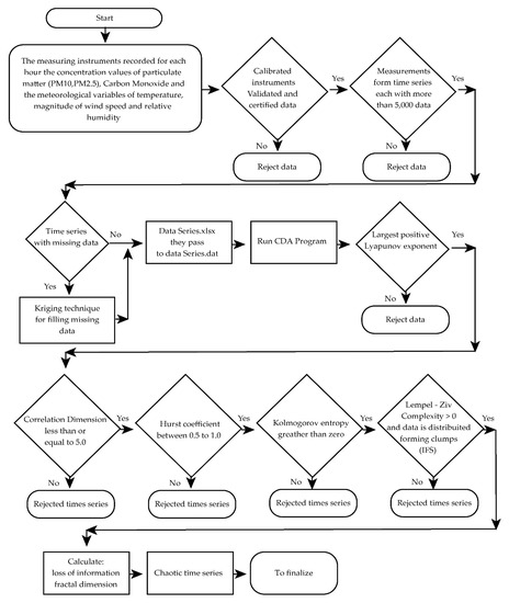
Figure 8. The flowchart describes the process that verifies the chaoticity of each series. The analysis is repeated for the six variables measured in each of the thirteen locations, giving a total of 78 time series.

Table 4 presents the results of the theory explained in Section 3.3 and summarized in the flowchart of Figure 8:

4. Results

4.1. Loss of Information and Fractal Dimension

Table 5 contains the calculation of the sum of information losses, <ΔI>, for pollutants and meteorological variables. With the exception of four locations, marked with * in Table 4, all the others show that the pollutants lose information faster than the meteorological variables. In the same way, Table 5 presents the fractal dimension for both systems of variables.

Table 5. It presents the sum of the information losses of the pollutants (P) and of the meteorological variables (MV). The fourth column gives the quotient between the losses of information between meteorological variables and pollutants. The last two columns show the fractional dimension of the pollutants and of the meteorological variables.

	Σ(<ΔI>)P	Σ(<ΔI>)MV	<ΔI>MV/<ΔI>P	DFP	DFMV
Basin:
Pudahuel	–2.89	−5.07	1.75	1.069	1.080
Kingst. Coll	−2.06	−6.45	3.13	1.094	1.100
Coyhaique *	−5.88	−3.51	0.60	1.094	1.126
Las Enc. Stat	−3.00	−8.75	2.92	1.089	1.111
Ent. Lag. Stat	−8.25	−9.50	1.15	1.199	1.119
Mex. Cty	−1.80	−4.50	2.50	1.073	1.024
Mountain:
Centro Stat	−3.50	−3.94	1.13	1.088	1.095
Tumbaco *	−6.64	−2.59	0.40	1.124	1.065
Carapungo *	−6.26	−2.74	0.44	1.110	1.064
Andac. Stat	−0.56	−3.97	7.09	1.094	1.071
Coast:
Con-Con Stat	−1.85	−5.67	3.07	1.064	1.109
Loncura Stat	−3.37	−4.72	1.40	1.117	1.070
Lot. Ru Stat *	−3.00	−1.97	0.66	1.108	1.102

On the other hand, Table 4 shows that in the meteorological variables the larger magnitudes of the Lempel–Ziv complexity depend on the location. Thus, for the basin, in most of the locations studied, the Lempel–Ziv complexity of Temperature and the magnitude of wind speed predominate [9] with slower loss of information. In Mountain, the Lempel–Ziv complexity that appears more dominant is that of the magnitude of the wind speed with slow loss of information. Additionally, on the coast it is the relative humidity, which also has a slow loss of information.

4.2. Entropy Quotient

Determination of C_K = S_{K, MET.VAR.}/S_{K, POLLUT} defined as the quotient between the sum of the entropies of pollutants with the sum of the entropies of the meteorological variables, values extracted from Table 4, for each locality.

(a)

Pudahuel is a commune in the interior of Santiago de Chile, the country’s capital and largest city. It is located in a valley surrounded by the Cordilleras de los Andes and the Coast (Figure 9):

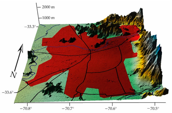Figure 9. C_{K, Pudahuel} = 0.98, the influence of the entropy of the contaminants is greater (Geographic coordinate system (GCS), World geodetic system 1984 (WGS84)).

(b)

Kingston College, environmental monitoring station, located in Concepción, a city with irregular geomorphology near the Cordillera of the Coast, marked by many geographical landmarks such as hills and depressions (Figure 10):

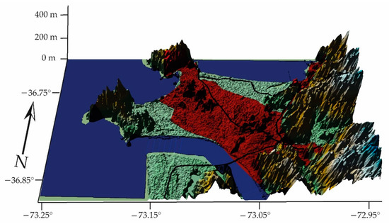Figure 10. C_{K, Kingston College} = 0.88, the influence of the entropy of the contaminants is greater (GCS, WGS84).

(c)

Coyhaique is located in the central zone of the Aysén Region at the foot of Cerro Mackay, to the east of the Cordillera de los Andes (part of it forms the Cerro Castillo range), in the place where the Simpson and Coyhaique rivers converge. Figure 10 is a representation of the geomorphology of the area (Figure 11):

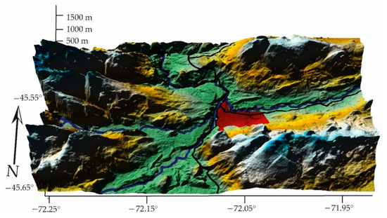Figure 11. Coyhaique Geomorphology, C_{K, Coyhaique} = 0.87 (GCS, WGS84).

(d)

Las Encinas station is in the city of Temuco, which is in a straight line 85.4 km from Puerto Saavedra, with access to the Pacific Ocean. It is located in the depression between the Cordillera de los Andes (highest peak, Lanín volcano, 3747 m above sea level) and the Cordillera of the Coast (highest peak, Cerro Alto Nahuelbuta, 1565 m above sea level) (Figure 12):

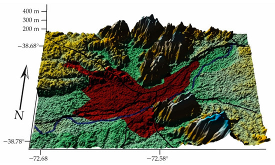Figure 12. C_{K, Las Encinas Stat} = 0.97, the entropy of the contaminants is more dominant (GCS, WGS84).

(e)

Entre Lagos station is located in the city of Osorno, 60.9 away from Bahía Mansa, access to the Pacific Ocean. It is located in the intermediate depression, between the Cordillera de los Andes (highest peak, Osorno volcano, 2660 masl) and the Cordillera of the Coast, low and undulating in the north, more robust in the south, exerting an effect of climatic screen in the intermediate depression (La Unión, Osorno and Río Negro) (Figure 13):

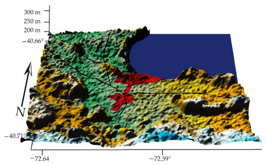Figure 13. C_{K, Entre Lagos Stat} = 0.97, pollutants affect local micrometeorology (GCS, WGS84).

(f)

Mexico City, located in a frank basin (a valley surrounded by heights), is circled by mountains that are part of the geological province of Anahuac Lakes and Volcanoes, forming the orographic cord of the capital (Figure 14):

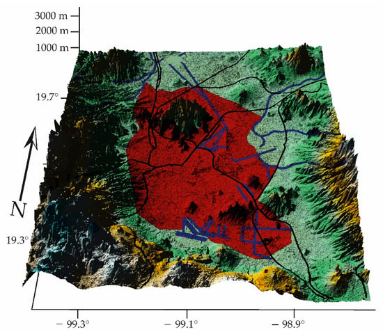Figure 14. C_{K, México City} = 0.35, the entropy of pollutants dominates the local micrometeorology (GCS, WGS84).

(g)

The Centro station is located within the commune of Calama, an inland and Andean city of Antofagasta (Figure 15):

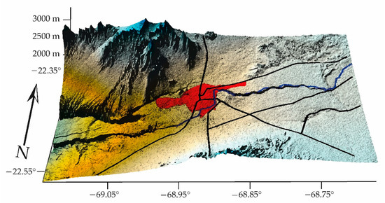Figure 15. C_{K, Centro Stat} = 1.60, local micrometeorological dominates pollutants (GCS, WGS84).

(h,i)

The Tumbaco and Carapungo stations are located in the interior of Quito, mountain cities of Ecuador (Figure 16).

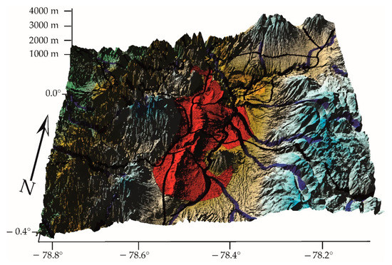Figure 16. Geomorphology of Quito, Ecuador, C_{K, Tumbaco} = 1.17, C_{K, Carapungo} = 1.40, local micrometeorology is superimposed on the effect of pollutants (GCS, WGS84).

(j)

The Andacollo station is located within the commune of the same name, Cordilleran city of Coquimbo (Figure 17):

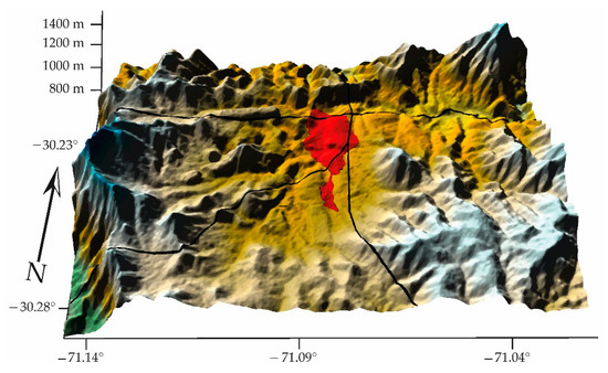Figure 17. Geomorphology of Andacollo, C_{K, Andacollo} = 4.46 (Pacheco et al., 2020) (GCS, WGS84).

(k)

The Concón station is located in the commune of the same name (Figure 18):

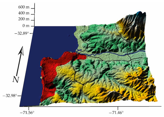Figure 18. C_{K, Concón} = 1.24, the activity of micrometeorology dominates that of pollutants (GCS, WGS84).

(l)

The Loncura station belongs to the commune of Quintero (Figure 19):

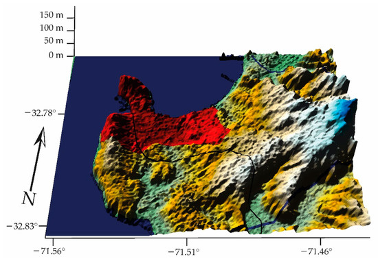Figure 19. C_{K, Loncura} = 1.66, micrometeorological activity dominates that of pollutants (GCS, WGS84).

(m)

The Lota Rural station is located in the district of Coronel (Figure 20):

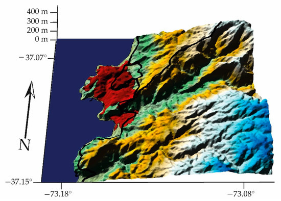Figure 20. Coronel Geomorphology, C_{K, Lota Rural} = 1.004 (GCS, WGS84).

Collecting the values of C_K = S_{K, MET.VAR.}/S_{K, POLUT}, the quotient between the sum of the entropies of pollutants with that of meteorological variables, by geographic morphology (Table 6):

Table 6. Summary of the ratios between the sum of the entropies of meteorological variables and the sum of the entropies of pollutants, C_K.

Morphology	Masl (m)	City	Σ Sk (Bits/h)P	Σ Sk (Bits/h)MV	CK
Basin (1)	2250	México, DF (1)	1.240	0.440	0.350
Basin (2)	469	Pudahuel (2)	1.030	1.020	0.980
Basin (3)	12	Kinston College (3)	0.900	0.800	0.880
Basin (4)	310	Coyhaique (4)	1.180	1.030	0.870
Basin (5)	360	Las Encinas (5)	1.200	1.170	0.970
Basin (6)	39	Entre Lagos (6)	1.780	1.740	0.970
Mountain (7)	2400	Centro Station (7)	0.760	1.230	1.600
Mountain (8)	1017	Andacollo Station (8)	0.200	0.870	4.460
Mountain (9)	2320	Tumbaco, Ecuador (9)	1.044	1.222	1.170
Mountain (10)	2697	Carapungo, Ecuador (10)	0.844	1.182	1.400
Coast (11)	2	Concón Station (11)	1.010	1.260	1.240
Coast (12)	3	Loncura (12)	0.820	1.360	1.660
Coast (13)	16	Lota Rural Station (13)	0.730	0.733	1.004

When plotting C_K according to urban settlements in various geographic morphologies of the study, numbered by (1), (2) … (13) (Figure 21):

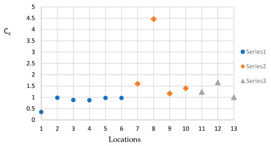
Figure 21. Quotient between entropies of meteorological variables and pollutant, C_K for cities in Cuenca (Series 1), Mountain (Series 2) and Coast (Series 3).

5. Discussion

In different geographic morphologies, the interaction of pollutants in the air with the section of the atmosphere closest to the earth’s surface, within the boundary layer, is studied. This layer can reach, during the day, a thickness of 1000 m, but at night it shrinks to a few dozen meters [6]. Hourly measurements of meteorological variables of temperature, relative humidity and magnitude of wind speed are used to characterize, as a first approximation, properties of the atmosphere. The same criterion of hourly measurable quantities is applied for pollutants PM₁₀, PM_2.5 and CO.

In total, we obtained 1,170,210 data from the 13 monitoring stations of the study, which correspond to measurements in the form of time series from different periods and locations. A numerical analysis method based on chaos theory is applied to each series, which allowed us to obtain seven chaotic parameters: Lyapunov Coefficient (λ > 0), Correlation Dimension (Dc < 5), Kolmogorov entropy (S_K > 0), Hurst exponent (0.5 < H < 1), Lempel–Ziv complexity (LZ > 0), fractal dimension (1 < D_F < 2) and information loss (⟨ΔI⟩ < 0), confirming the chaotic nature of each time series [44] and the complexity of the analyzed system.

Using the series and its seven chaotic parameters [47], its relationship with three geographic morphologies was studied. In particular, for each location, an indicator defined as the quotient (C_K) between the entropies of the meteorological variables and those of the pollutants, C_{K, LOCATION} = (S_{K, MET.VAR.}/S_{K, POLLUTANTS}) _{BY LOCATION}, was constructed.

The locations in high mountains and coastal sectors show that the atmospheric system, characterized by the indicated meteorological variables, achieves a better dispersion of pollutants, promoting a relatively cleaner atmospheric layer, with a domain of local meteorology [62]. This is not a solution to the problem of atmospheric contamination of the boundary layer; it is an attenuation in the measurement location and a transfer of contaminants to other areas.

Table 4 presents the Hurst coefficient (H). These coefficients show that in the basin, the pollutant concentration time series are more persistent, which means that they have a greater capacity to influence the future. This is different in the mountains and on the coast, where the Hurst coefficients of the meteorological variables predominate, influencing the future, favoring a cleaner atmosphere. This methodology allows us to infer results that have been obtained using wind flow analysis methods.

The fractal dimension (D_F = 2 − H) associated with meteorological variables and pollutants depends on the geographic morphology. In the case of Cuenca, four of the six localities comply with D_FMV > D_FP; in the case of mountains, three of the four locations meet D_FP > D_FMV; in the case of the coast, two of the three locations studied meet D_FP > D_FMV. The fractal dimension can be related to the degree of roughness that the time series presents, where the meteorology and pollutant data were measured at the level of ground that has geometry of highly variable height, which shows that the series is “sensitive” to the registration and description of highly complex objects.

The analysis of measurements of meteorological variables at a scale very close to the ground shows high turbulence [29] due to the pronounced change in surface roughness, due to human activity, in the three morphologies studied. In 70% of the total morphologies studied, the meteorological variables present Lempel–Ziv complexity higher than that of the pollutants, which is proof of their connectivity, in a disturbed atmospheric layer, with the change in roughness. The fractal dimension in the basin, greater in the meteorological variables, confirms that these series record events that have become more turbulent due to intensive soil modification. The persistence of the meteorological variables in the basin is greater compared to that of the pollutants in the mountains and on the coast (five out of seven localities), which translates into a greater capacity to influence the future. This is consistent with the fact that the fractal dimension of the meteorological variables, in five of the seven coastal and mountain locations studied (Table 5), is lower compared to that of the pollutants, which are less persistent and more chaotic and influenced by urban meteorology, which is unstable, but more robust.

There are other factors [9] that can contribute to the roughness of the series. There is a long drought, in the context of global climate change, that affects the central zone of Chile [63], altering the localized micrometeorology. This has an effect on the series, as do intensive urbanization and densification processes, by causing substantial changes in surface roughness. This work shows that the atmospheric boundary layer, immediately next to this artificial roughness of increasing height, is less and less resilient, being dominated by regimes of extreme persistence of pollutants or meteorological variables. The last case generates an appearance of mitigation of contaminants.

The urbanization of extensive surfaces must take into account the characteristics of its geography, the meteorology of its boundary layer, the concentrations of pollutants (present and projected) and the interaction between these three elements. The results show that a strategy of increasing urban densification is not sustainable [59,64,65,66,67,68]. As can be deduced from this study, the location of human settlements has a great effect on the local climatology, even more so in areas that exhibit extreme fragility due to water deficit [63], given their natural connectivity at all levels [65].

Interacting with the natural microclimate, artificial contents coexist, referring to human activities. The chaotic analysis applied in this study reveals the interaction between pollutants and their effect on the historical regularity of meteorological parameters such as relative humidity, temperature and magnitude of wind speed. The qualitative model elaborated reveals, using direct measurements; the gap between the processes associated with pollutants and those of the urban microclimate [9] in the different morphologies presented the most vulnerable. This allows comparison with remote sensing measurements [68,69] based on the digital interpretation of data.

This research reveals that at the microscale, urban meteorology and pollutants behave turbulently in all geographic morphologies, and the time series are chaotic, which can be interpreted as a Kolmogorov cascade manifestation [9,70]. Flows in the atmosphere very close to the Earth’s surface have turbulent and dissipative characteristics. In these smaller scales, the viscosity of the medium enables the dissipation of the kinetic energy received in cascade from the larger scales (higher heights of the boundary layer). This dissipated kinetic energy manifests itself as heat, which is directly related to the entropy acquired by the system, which can be decisive for the establishment of thermal islands. There is much evidence of the influence of artificial climatology over the natural one. It is known that it generates thermal islands that can alter thermal fluxes [59,63], especially in countries with complex geomorphological characteristics and precarious climatic conditions.

The relevance of this study is that it shows, in a unified way, the connectivity between various areas such as geography, urban planning, meteorology, pollutants produced by human activity, epidemiology [17,71,72], etc., expanding the connectivity towards geomorphology.

6. Conclusions

From the chaotic analysis of experimental time series, urban meteorology and atmospheric pollutants, measured at ground level in three geographical morphologies (basin, mountain, coast), it is concluded:

The Lyapunov exponent of the time series of meteorological variables, in 70% of the locations, is greater than that of the time series of pollutants (basin: 5/6 locations, mountain: 2/4 locations and coast: 2/3) which indicates high chaoticity in urban meteorology.

Of all the localities studied in basin morphology, it was found that the urban meteorology of most of them has a higher fractal dimension than that of the pollutants. The change in roughness plus the boxing of the city favors its complexity, since these localities also have greater Lempel–Ziv complexity. In the case of mountains and coasts, it was determined that for the set of localities studied, the fractal dimension of the pollutants is greater than that of urban meteorology, which has, comparatively, a higher Lempel–Ziv complexity. These geographic morphologies are open and sensitive to wind (mountain: two localities out of four with high complexity) and relative humidity (coast: three localities out of three with high complexity).

The loss of information of the contaminants is faster than that of the meteorological variables in the basin. This is due to the enclosing and the intensity of the contaminating activities permanently receiving new information. In the mountains and coasts, the opposite occurs: urban meteorology loses information faster given its nature of open spaces.

The resulting entropy of the measured pollutants is greater than the resulting entropy of the meteorological variables measured in the basin. It happens the other way around in the mountains and on the coast. This favors the suggestion that mountains and coasts are more ventilated with respect to the concentration of pollutants.

The ratio between Kolmogorov entropies of meteorological variables (T, HR and VV) and of selected pollutants (PM_2.5, PM₁₀, CO) can be used, in a first approximation criterion, as a discriminant of the effect of pollutants on local meteorology:

$$\frac{{\mathrm{S}}_{\mathrm{K}, \mathrm{MET}.\mathrm{VAR}.}}{{\mathrm{S}}_{\mathrm{K}, \mathrm{POLLUT}}}=\{\begin{array}{c}<1, \mathrm{case}1 \mathrm{cities} \mathrm{in} \mathrm{basin}\hfill \\ >1, \mathrm{case} 2 \mathrm{high} \mathrm{mountain} \mathrm{cities}\hfill \\ >1, \mathrm{case} 3 \mathrm{coastal} \mathrm{cities}\hfill \end{array}$$

The selection of geographic morphologies for urban settlements, with the consequent human activity and change in surface roughness, has a high impact on the atmosphere. The urban climate that will develop will connect with everything that surrounds it. Geographic morphologies and the atmosphere are sensitive to changes in initial conditions, and entropy allows us to qualitatively visualize the different responses using urban meteorology and atmospheric pollutants. The temporal scales of human activity do not collaborate in this process, since they do not contribute to resilience or observable atmospheric sustainability in the criteria of this study.

References

- Girardet, H. Cities People Planet: Liveable Cities for a Sustainable World; Earthscan: London, UK, 2004. [Google Scholar]
- Delgado, G.C. Geoingeniería, apuesta incierta frente al cambio climático. Estud. Soc. 2012, 20, 213–236. [Google Scholar] [CrossRef]
- Hernàndez, J.M. Cambio Climático y Geología. Interacciones y Consecuencias a Escala Local y Global. Communicational Strategy against the Climate Change in the City of San Sebastian. 2016. Available online: www.conama2016.org (accessed on 10 December 2021).
- Cárdenas-Jirón, L.-A.; Morales-Salinas, L. Urbanismo bioclimático en Chile: Propuesta de biozonas para la planificación urbana y ambiental. EURE 2019, 45, 135–162. [Google Scholar] [CrossRef]
- Bettini, V. Elementos de Ecología Urbana. In Serie Medio Ambiente; Trotta: Madrid, Spain, 1998. [Google Scholar]
- Stull, R.B. Meteorology for Scientists and Engineers, 2nd ed.; Brooks/Cole: Pacific Grove, CA, USA, 2000. [Google Scholar]
- Mauree, D.; Naboni, E.; Coccolo, S.; Perera, A.; Nik, V.M.; Scartezzini, J.-L. A review of assessment methods for the urban environment and its energy sustainability to guarantee climate adaptation of future cities. Renew. Sustain. Energy Rev. 2019, 112, 733–746. [Google Scholar] [CrossRef]
- Dennis, M.; Scaletta, K.L.; James, P. Evaluating urban environmental and ecological landscape characteristics as a function of landsharing-sparing, urbanity and scale. PLoS ONE 2019, 14, e0215796. [Google Scholar] [CrossRef] [PubMed]
- Pacheco, P.; Mera, E.; Salini, G. Urban Densification Effect on Micrometeorology in Santiago, Chile: A Comparative Study Based on Chaos Theory. Sustainability 2022, 14, 2845. [Google Scholar] [CrossRef]
- Sharples, S.; Lash, D. Daylight in Atrium Buildings: A Critical Review. Arch. Sci. Rev. 2007, 50, 301–312. [Google Scholar] [CrossRef]
- Du, J.; Sharples, S. An Analysis of Vertical Daylight Level Distributions across the Walls of Atria. In Proceedings of the CIE 2010: Lighting Quality & Energy Efficiency, Vienna, Austria, 14–17 March 2010; Volume 1. Available online: https://www.researchgate.net/publication/335565925 (accessed on 22 January 2022).
- Aguilar, G.; Riquelme, R.; Martinod, J.; Darrozes, J. Role of climate and tectonics in the geomorphologic evolution of the Semiarid Chilean Andes between 27-32 °S. Andean Geol. 2013, 40, 79–101. [Google Scholar] [CrossRef]
- Belušić, D.; Hrastinski, M.; Večenaj, Ž.; Grisogono, B. Wind Regimes Associated with a Mountain Gap at the Northeastern Adriatic Coast. J. Appl. Meteorol. Clim. 2013, 52, 2089–2105. [Google Scholar] [CrossRef]
- Strahler, A.N. Physical Geography; John Wiley & Sons: New York, NY, USA, 1960. [Google Scholar]
- O’Connor, J.J.; Robertson, E.F. Evangelista Torricelli. MacTutor History of Mathematics and Science. 2002. Available online: http://www-history.mcs.st-and.ac.uk/Biographies/Torricelli.html (accessed on 30 July 2021).
- Toledano, C. Los Aerosoles Atmosféricos y su Influencia en la Península Ibérica. Manual Formativo de ACTA Nº 48. 2008. Available online: https://dialnet.unirioja.es/servlet/articulo?codigo=509874621/06/2019 (accessed on 14 February 2022).
- Ilabaca, M.; Olaeta, I.; Campos, E.; Villaire, J.; Tellez-Rojo, M.M.; Romieu, I. Association between levels of fine particulate and emergency visits for pneumonia and other respiratory illnesses among children in Santiago, Chile. J. Air Waste Manag. Assoc. 1999, 49, 154–163. [Google Scholar] [CrossRef] [PubMed]
- Bełcik, M.; Trusz-Zdybek, A.; Zaczyńska, E.; Czarny, A.; Piekarska, K. Genotoxic and cytotoxic properties of PM2.5 collected over the year in Wrocław (Poland). Sci. Total Environ. 2018, 637–638, 480–497. [Google Scholar] [CrossRef] [PubMed]
- Jia, Y.; Schmid, C.; Shuliakevich, A.; Hammers-Wirtz, M.; Gottschlich, A.; der Beek, T.A.; Yin, D.; Qin, B.; Zou, H.; Dopp, E.; et al. Toxicological and ecotoxicological evaluation of the water quality in a large and eutrophic freshwater lake of China. Sci. Total Environ. 2019, 667, 809–820. [Google Scholar] [CrossRef] [PubMed]
- Schwartz, J.; Laden, F.; Zanobetti, A. The concentration-response relation between PM2.5 and daily deaths. Environ. Health Perspect. 2002, 110, 1025–1029. [Google Scholar] [CrossRef] [PubMed]
- Raabe, O.G. Respiratory exposure to air pollutants. In Air Pollutants and the Respiratory Tract; Swift, D.L., Foster, W.M., Eds.; Taylor and Francis: Boca Ratón, CA, USA, 2005; pp. 39–74. [Google Scholar]
- Reyna, M.A.; Mérida, J.V.; Osornio-Vargas, A.R.; Lerma, C.; Bravo-Zanoguera, M.E.; Avitia, R.L.; Nieblas, E.C. Association between personal PM10 exposure and pulmonary function in healthy volunteers from a semi-arid city on the US-Mexican border. Rev. Int. Contam. Ambient. 2018, 34, 583–585. [Google Scholar] [CrossRef]
- Peters, A.; Dockery, D.W. Lung Biology in Health and Disease. In Air Pollutants and the Respiratory Tract; Foster, W.M., Costa, D.L., Eds.; CRC Press: Boca Raton, CA, USA, 2005; pp. 1–20. [Google Scholar]
- Cifuentes, L.A.; Vega, J.; Köpfer, K.; Lave, L.B. Effect of the Fine Fraction of Particulate Matter versus the Coarse Mass and Other Pollutants on Daily Mortality in Santiago, Chile. J. Air Waste Manag. Assoc. 2000, 50, 1287–1298. [Google Scholar] [CrossRef] [PubMed]
- Lee, B.-J.; Kim, B.; Lee, K. Air Pollution Exposure and Cardiovascular Disease. Toxicol. Res. 2014, 30, 71–75. [Google Scholar] [CrossRef]
- Santiago, J.; Sanchez, B.; Quaassdorff, C.; de la Paz, D.; Martilli, A.; Martín, F.; Borge, R.; Rivas, E.; Gómez-Moreno, F.; Díaz, E.; et al. Performance Evaluation of a Multiscale Modelling System Applied to Particulate Matter Dispersion in A Real Traffic Hot Spot in Madrid (Spain). Atmospheric Pollut. Res. 2019, 11, 141–155. [Google Scholar] [CrossRef]
- Farmer, J.D. Chaotic attractors of an infinite-dimensional dynamical system. Phys. D Nonlinear Phenom. 1982, 4, 366–393. [Google Scholar] [CrossRef]
- Farmer, J.D.; Otto, E.; Yorke, J.A. The dimension of chaotic attractors. Physica D 1983, 7, 153–180. [Google Scholar] [CrossRef]
- Kolmogorov, A.N. On entropy per unit time as a metric invariant of automorphisms. Dokl. Akad. Nauk SSSR 1959, 124, 754–755. [Google Scholar]
- Martínez, J.A.; Vinagre, F.A. La Entropía de Kolmogorov; su Sentido Físico y su Aplicación al Estudio de Lechos Fluidizados 2D; University of Alcalá: Alcalá de Henares, Madrid, 2016; Available online: https://www.academia.edu/2479372/LA_ENTROP%C3%8DA_DE_KOLMOGOROV_SU_SENTIDO_F%C3%8DSICO_Y_SU_APLICACI%C3%93N_AL_ESTUDIO_DE_LECHOS_FLUIDIZADOS_2D (accessed on 29 January 2022).
- Shannon, C. A mathematical theory of communication. Bell Syst. Technol. J. 1948, 27, 379–423, 623–656. [Google Scholar] [CrossRef]
- Brillouin, L. Science and Information Theory, 2nd ed.; Academic Press: New York, NY, USA, 1962; 304p. [Google Scholar]
- Shaw, R. Strange attractors, chaotic behavior and information flow. Zeitschrift für Naturforschung A 1981, 36, 80–112. [Google Scholar] [CrossRef]
- Cohen, A.; Procaccia, I. Computing the Kolmogorov entropy from time signals of dissipative and conservative dynamical systems. Phys. Rev. A 1985, 31, 1872–1882. [Google Scholar] [CrossRef] [PubMed]
- SINCA. Chile, Sistema de Información Nacional de Calidad del Aire. 2022. Available online: https://sinca.mma.gob.cl/ (accessed on 23 April 2022).
- SINAICA. Mexico, Sistema Nacional de Información de la Calidad del Aire. 2022. Available online: https://sinaica.inecc.gob.mx/ (accessed on 12 February 2022).
- SUIA. Ecuador, Sistema Único de Información Ambiental. 2022. Available online: http://suia.ambiente.gob.ec/ambienteseam/home.seam (accessed on 2 January 2022).
- Norazian, M.N.; Shruki, Y.A.; Azam, R.M.; Mustafa Al Bakri, A.M. Estimation of missing values in air pollution data using single imputation techniques. ScienceAsia 2008, 34, 341–345. [Google Scholar] [CrossRef]
- Junninen, H.; Niska, H.; Tuppurainen, K.; Ruuskanen, J.; Kolehmainen, M. Methods for imputation of missing values in air quality data sets. Atmos. Environ. 2004, 38, 2895–2907. [Google Scholar] [CrossRef]
- Salini, G.A.; Medina, E. Estudio sobre la dinámica temporal de material particulado PM10 emitido en Cochabamba, Bolivia. Rev. Int. Contam. Ambient. 2017, 33, 437–448. [Google Scholar] [CrossRef][Green Version]
- Asa, E.; Saafi, M.; Membah, J.; Billa, A. Comparison of linear and nonlinear Kriging methods for characterization and interpolation of soil data. J. Comput. Civil Eng. 2012, 26, 11–18. [Google Scholar] [CrossRef]
- Emery, X. Simple and Ordinary Multigaussian Kriging for Estimating Recoverable Reserves. Math. Geol. 2005, 37, 295–319. [Google Scholar] [CrossRef]
- Kyriakidis, P.; Journel, A. Geostatistical space-time models: A review. Math. Geol. 1999, 6, 651–684. [Google Scholar] [CrossRef]
- Kantz, H.; Schreiber, T. Nonlinear Time Series Analysis, 2nd ed.; Cambridge University Press: Cambridge, UK, 2004; 387p. [Google Scholar]
- Sivakumar, B.; Wallender, W.W.; Horwath, W.R.; Mitchell, J.P. Nonlinear deterministic analysis of air pollution dynamics in a rural and agricultural setting. Adv. Complex Syst. 2007, 10, 581–597. [Google Scholar] [CrossRef]
- Sprott, J.C. Chaos Data Analyzer Software. 1995. Available online: http://sprott.physics.wisc.edu/cda.htm (accessed on 1 April 2022).
- Sprott, J.C. Chaos and Time-Series Analysis; Oxford University Press: Oxford, UK, 2003; 528p. [Google Scholar]
- Lorenz, E. Deterministic nonperiodic flow. J. Atmos. Sci. 1963, 20, 130–141. [Google Scholar] [CrossRef]
- Kumar, U.; Prakash, A.; Jain, V.K. Characterization of chaos in air pollutants: A Volterra-Wiener-Korenberg series and numerical titration approach. Atmos. Environ. 2008, 42, 1537–1551. [Google Scholar] [CrossRef]
- Lee, C.-K.; Lin, S.-C. Chaos in Air Pollutant Concentration (APC) Time Series. Aerosol Air Qual. Res. 2008, 8, 381–391. [Google Scholar] [CrossRef]
- Salini, G.; Pérez, P. A study of the dynamic behavior of fine particulate matter in Santiago, Chile. Aerosol Air Qual. Res. 2015, 15, 154–165. [Google Scholar] [CrossRef]
- Takens, F. Detecting Strange Attractors in Turbulence. In Dynamical Systems and Turbulence, Warwick 1980; Springer: Berlin/Heidelberg, Germany, 1981; pp. 366–381. [Google Scholar]
- Fraser, A.M.; Swinney, H.L. Independent coordinates for strange attractors from mutual information. Phys. Rev. A 1986, 33, 1134–1140. [Google Scholar] [CrossRef] [PubMed]
- Calderón, G.S.; Jara, P.P. estudio de series temporales de contaminación ambiental mediante técnicas de redes neuronales artificiales. Ingeniare 2006, 14, 284–290. [Google Scholar] [CrossRef][Green Version]
- Eckmann, J.P.; Oliffson, S.; Kamphorst, S.; Ruelle, D.; Ciliberto, C. Lyapunov exponents from time series. Phys. Rev. A 1986, 34, 4971–4979. [Google Scholar] [CrossRef]
- Grassberger, P.; Procaccia, L. Characterization of strange attractors. Phys. Rev. Lett. 1983, 50, 346–349. [Google Scholar] [CrossRef]
- Wolf, A.; Swift, J.B.; Swinney, H.L.; Vastano, J.A. Determining Lyapunov exponents from a time series. Phys. D 1985, 16, 285–317. [Google Scholar] [CrossRef]
- Gao, J.; Cao, Y.; Tung, W.-W.; Hu, J. Multiscale Analysis of Complex Time Series; Wiley and Sons Interscience: Hoboken, NJ, USA, 2007; 368p. [Google Scholar]
- Hernández, P.R.P.; Calderón, G.A.S.; Garrido, E.M.M. Entropía y neguentropía: Una aproximación al proceso de difusión de contaminantes y su sostenibilidad. Rev. Int. Contam. Ambient. 2021, 37, 167–185. [Google Scholar] [CrossRef]
- Chelani, A.B.; Devotta, S. Nonlinear analysis and prediction of coarse particulate matter concentration in ambient air. J. Air Waste Manag. Assoc. 2006, 56, 78–84. [Google Scholar] [CrossRef][Green Version]
- Horna, J.; Dionicio, J.; Martínez, R.; Zavaleta, A.; Brenis, Y. Dinámica simbólica y algunas aplicaciones. Sel. Mat. 2016, 3, 101–106. [Google Scholar] [CrossRef]
- Pacheco, P.R.; Parodi, M.C.; Mera, E.M.; Salini, G.A. Variables meteorológicas y niveles de concentración de material particulado de 10 μm en Andacollo, Chile: Un estudio de dispersión y entropías. Inform. Tecnol. 2020, 31, 171–182. [Google Scholar] [CrossRef]
- Araya-Osses, D.; Casanueva, A.; Román-Figueroa, C.; Uribe, J.M.; Paneque, M. Climate change projections of temperature and precipitation in Chile based on statistical downscaling. Clim. Dyn. 2020, 54, 4309–4330. [Google Scholar] [CrossRef]
- Borrego, C.; Rafael, S.; Rodrigues, V.; Monteiro, A.; Sorte, S.; Coelho, S.; Lopes, M. Air Quality, Urban Fluxes and Cities Resilience Under Climate Change—A Brief Overview. Int. J. Environ. Impacts 2018, 1, 14–27. [Google Scholar] [CrossRef]
- Balaban, O. The negative effects of construction boom on urban planning and environment in Turkey: Unraveling the role of the public sector. Habitat Int. 2012, 36, 26–35. [Google Scholar] [CrossRef]
- Munir, S.; Mayfield, M.; Coca, D.; Mihaylova, L.S.; Osammor, O. Analysis of Air Pollution in Urban Areas with Airviro Dispersion Model—A Case Study in the City of Sheffield, United Kingdom. Atmosphere 2020, 11, 285. [Google Scholar] [CrossRef]
- Coseo, P.; Larsen, L. How factors of land use/land cover, building configuration, and adjacent heat sources and sinks explain Urban Heat Islands in Chicago. Landsc. Urban Plan. 2014, 125, 117–129. [Google Scholar] [CrossRef]
- Huang, X.; Wang, Y. Investigating the effects of 3D urban morphology on the surface urban heat island effect in urban functional zones by using high-resolution remote sensing data: A case study of Wuhan, Central China. ISPRS J. Photogramm. Remote Sens. 2019, 152, 119–131. [Google Scholar] [CrossRef]
- Kadygrov, E.N.; Shur, G.N.; Viazankin, A.S. Investigation of atmospheric boundary layer temperature, turbulence, and wind parameters on the basis of passive microwave remote sensing. Radio Sci. 2003, 38, 8048. [Google Scholar] [CrossRef]
- Kolmogorov, A.N. The local structure of turbulence in incompressible viscous fluid for very large Reynolds numberst, Dokl. Akad. Nauk. SSSR 1941, 30, 301–305. [Google Scholar]
- Pacheco, P.; Mera, E. Study of the Effect of urban densification and micrometeorology on the sustainability of a coronavirus-type pandemic. Atmosphere 2022, 13, 1073. [Google Scholar] [CrossRef]
- MMA (Ministerio del Medioambiente de Chile). Sistema de Información Nacional de Calidad del Aire. 2021. Available online: https://mma.gob.cl/ (accessed on 30 April 2021).
Publisher’s Note: MDPI stays neutral with regard to jurisdictional claims in published maps and institutional affiliations. |
© 2022 by the authors. Licensee MDPI, Basel, Switzerland. This article is an open access article distributed under the terms and conditions of the Creative Commons Attribution (CC BY) license (https://creativecommons.org/licenses/by/4.0/).