Abstract
The accurate identification of ozone (O3) production sensitivity is central to developing O3 pollution control policies. It is determined by the relative ratio of the radical loss to the total primary radical production. However, such radical losses in the traditional sensitivity analysis typically rely on nitrogen oxide (NOx) sinks while ignoring particle uptake (collisions between compounds in the gas phase and condensed phases that result in irreversible uptake due to chemical reactions). Therefore, we combine NOx and particle uptakes to optimize peroxy radical loss estimates and thus analyze the relative sensitivity. We also assess the absolute responses of precursor reduction to O3 production. Such relative and absolute sensitivity analysis is applied to measurements in Chun’an, a county in China, where volatile organic compounds (VOCs) and NOx are both rich. Consequently, the relative sensitivity analysis presents that the dominant precursor for O3 production sensitivity shifts from volatile organic compounds (VOCs) in the morning and evening to NOx in the afternoon, the main driver of which is related to NO depletion. In contrast, the absolute sensitivity analysis confirms that VOCs persistently determine the diurnal ozone production sensitivity. Moreover, they both show that particle uptake does not change the regime classification of O3 production sensitivity (i.e., VOC- or NOx-sensitive regime) but potentially has a strong inhibition on the sensitivity magnitude (within 16% and 38% for VOC- or NOx-sensitive regimes, respectively). Our results partly explain more insensitive O3 production measurements than those suggested by traditional sensitivity analyses, which has important implications for synergistic controls on O3 and fine particulate matter pollution.
1. Introduction
Tropospheric ozone (O3) plays a central role in photochemical oxidation. High levels of tropospheric O3 adversely affect human health, ecosystems, and climate change [1,2,3,4,5]. O3 concentrations regularly exceed China’s Ambient Air Quality Standard in nearly every season nationwide. Tropospheric O3 is formed photochemically via its precursors: volatile organic compounds (VOCs) and nitrogen oxides (NOx ≡ NO + NO2). It is well established that O3 production depends on VOCs and NOx availability. A classic isopleth diagram applies a distinctive ridge to separate O3 production sensitivity into two regimes: a VOCs-sensitive regime with abundant NOx budgets and a NOx-sensitive regime with sufficient VOC budgets [6]. As such, in the NOx-sensitive regime, reducing NOx budgets can effectively affect O3 production, while reducing O3 production might run counter to our desire. Therefore, the accurate identification of O3 production sensitivity is central to developing O3 pollution control policies.
The O3 formation sensitivity analysis is typically a function of the fraction of radicals lost in the radicals + NOx reactions. This proportion is designated as (LN/Q) and is determined for each sample as the ratio of the loss rate from the R + NOx reactions (LN) to the overall radical production rate (Q). When LN/Q is significantly less than 0.5, the O3 formation sensitivity is in a NOx-sensitive regime. In contrast, the O3 formation sensitivity is in a VOCs-sensitive regime [7,8,9,10]. A classic theory suggests that particle uptake has the potential to affect the peroxy radical loss, for which, however, theoretical sensitivity analysis typically makes no allowance. Model studies have shown that particle uptake might account for 10~40% of the peroxy radical concentrations. It could compete with the NOx reactions, influencing the O3 sensitivity regime and production rates.
Note that the uptake coefficient (the fraction of molecules that do not return to the gas phase after a collision with the surface) of the radical loss varies depending on factors, such as meteorological conditions, particle concentration, and mixing states [11]. Previous measurements and modeling studies have confirmed that this ratio fluctuates widely, e.g., more than 0.2 for liquid particles and less than 0.002 for dry particles [12,13]. So far, there remains a very limited sampling dataset for real-world uptake coefficients. To our knowledge, particle phase changes might lead to a high uptake coefficient of roughly 0.2. Furthermore, considering other situations, such as relative humidity, temperature, and particle concentrations, can lead to more accurate predictions of the uptake coefficient [14]. Otherwise, a large bias may arise when employing a constant value. Consequently, observation-based ensemble sensitivity analysis might be necessary to assess the impacts of particle uptake on the peroxy radical loss and subsequent O3 production sensitivity.
To date, field campaigns have been one of the most effective ways of addressing the above issue. They could track the daytime variations in the regimes of O3 production sensitivity and thus identify whether either VOCs or NOx reductions dominate O3 mitigation over a given time window. Such explorations, while attempted for megacities, remain unclear in the suburbs [15]. A huge number of field campaigns and laboratory studies have better characterized the concentrations of VOCs and NOx, which both differ from the urban cases [16,17]. Particularly, biogenic VOCs are rich due to abundant local emissions, while NOx might not fall as much as biogenic VOCs rise due to downwind impacts [18]. Moreover, the relationships among VOCs, NOx, and O3 can differ sharply during different periods [19,20,21]. However, in such cases, the impacts of particle uptake are not considered comprehensively.
Here, we take both NOx sinks with particle uptake into account to optimize the observation-based analysis of the radical loss, and thus, O3 relative production sensitivity. We also introduce the absolute responses of O3 precursor reduction to O3 production (i.e., absolute sensitivity analysis). This allows us to assess the efficiency and variability of precursor reduction in O3 reductions across a specific spatiotemporal scale. This relative and absolute sensitivity analysis is applied to long-term measurements in Chun’an, a county in China, where O3 precursors and particles are both rich. We also compare this sensitivity analysis to traditional sensitivity indicators such as [HCHO]/[NO2] [22,23] and [NMHC]/[NOx] [15,24,25]. Our results have the potential to offer synergistic controls on O3 and fine particulate matter pollution.
2. Materials and Methods
2.1. Ozone Sensitivity Analysis
The theoretical foundation of the O3 sensitivity analysis is the chemical reaction cycle of the radical, as illustrated in Figure 1 [26]. First, the sole critical source of troposphere O3 comes from the reaction of NO with peroxy radicals () (Equations (1) and (2)).
where represents the output organic nitrate (). According to the classic theory [7], it is thought to be insignificant and would thus be ignored in the following derivation ().
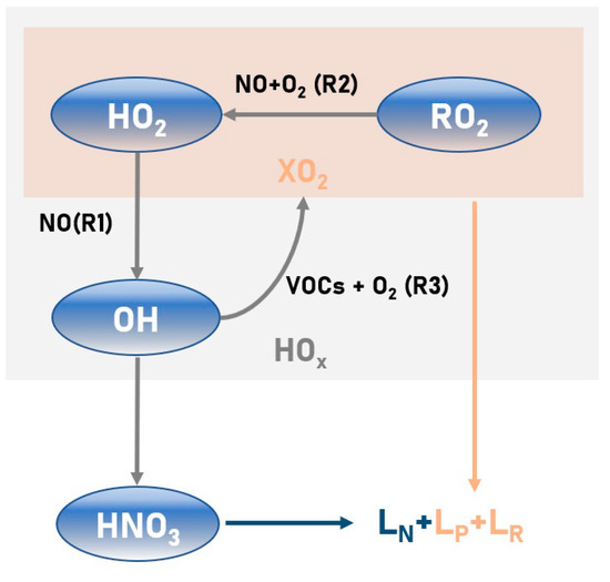
Figure 1.
Theoretical framework of the HOx radical cycle. This framework considers the rates of radical losses due to particle uptakes (), peroxide formation (), and reactions (). Mainly, the reaction of NO with the peroxy radicals () (Equations (1) and (2)) and the reaction of OH with VOCs (Equation (3)) are included.
Secondly, OH would react with VOCs to yield (Equation (3)).
On this basis, the chemical reaction cycle of the radical is born (Equations (1)–(3)). We could thus express the rate of O3 production as (Equation (4)).
It is clear that equals , while and serve as the second-order reaction coefficients for Equations (1) and (2), respectively. Consequently, the whole rate of the radical cycle () must consider the rates of radical losses due to particle uptakes (), peroxide formation (), and reactions (), which are expressed as follows.
Specifically, for , the rate constants for () and () are considered separately.
We assume that is nearly determined by the radical cycle, which could thus be regarded as a function of , [], and [] as follows.
where denotes the reaction rate constant, and equals []/[]. Following Equation (3), we define as the overall reactivity that contains the reactions with and .
For the last radical loss rate (), the distinctive calculation in this study, the rate constants for () and () are both considered.
These rate constants ( and ) are closely related to the particle surface areas (), the thermal mean velocity (), and the corresponding effective uptake coefficients (, i.e., or ) [27]. We thus take these factors into account to make reliable estimates for and .
Note that we need to correct these uptake coefficients () for gas phase diffusion. The resistance model defines conductance as the rate of each process normalized to the gas–surface collision rate. This suggests these uptake coefficients follow the law involving the conductance values for gas phase diffusion () and other processes () [6]:
A classic study [28] proposed a relationship between and by approximating the independence of from :
where, at a given radius (), and represent the surface area distribution function and Knudsen number, respectively. The latter depends on the mean thermal velocity () and the gas phase diffusion constant ().
As abovementioned, the traditional relative sensitivity analysis (i.e., the relative change in ) considers only the relative variation in [VOCs] or [NOx], excluding [7]. In theory, depending on the particle characteristics [24], plays a key role in affecting the radical loss. Here, we expand the sensitivity analysis by introducing to investigate the possible influence.
When , as proposed by Kleinman et al. [7], the relative sensitivity refers to the percent change in [VOCs] or [NOx], which is a function of as follows.
In contrast, when LP >> LR, we combine Equations (4), (6), (7), (9), and (10) to re-express and as follows.
In this case, is independent of the precursor concentration change. The relative sensitivity is as follows.
Moreover, by differentiating Equation (8) E5, we can get:
Substituting Equations (23) and (24) into Equations (21) and (22) provides Equations (25) and (26).
Collectively, whether LP >> LR (Equation (25)) or LR >> LP (Equation (26)), the relative O3 sensitivity () follows a function of (Figure S1). Specifically, when LP >> LR, the turning point () between NOx-sensitive and VOC-sensitive regimes is at 1/3, while the zero-crossing point () is at 1/2. In turn, when LR >> LP, and are 1/2 and 2/3, respectively, in the previous treatment [7,8].
When or , the relative O3 sensitivity () should be between the above extremes. At this moment, it is assumed to follow a linear combination of Equations (15) and (25) using a branching ratio ().
Hence, and indicate Equation (26) = Equation (27) and Equation (26) = 0.
We can thus apply to express both equations approximately.
Figure S2 confirms that this linear idealization using can reproduce the analytical (Equation (29)) and (Equation (30)).
In addition, considering the radical loss by uptake onto particles, we define as follows.
First, Equation (8) E5 results in:
Second, by substituting Equations (7) and (8) into (6), we obtain [XO2]:
Third, we assume that the reaction cycle is of sufficient radical propagation.
Finally, we combine Equations (33), (34), and (5) to resolve :
Consequently, given that the intermediate case covers the extreme case (i.e., LP >> LR or LR >> LP), this work adopted Equations (27), (28), (31), and (36) for the subsequent sensitivity analysis. Such equations and parameters are summarized in Table S1. Note that the values for ], , and were not observed in this field campaign and thus refer to previous findings. Specifically, we refer to the function between [] and ] in the previous study [8]. The typical value () was used [29]. According to common model configurations, we set and to 0.2 and 0, respectively [29].
In this work, we also designed a concept of the absolute sensitivity analysis. It relies on the multiplication of with the relative sensitivity.
where represents NOx or VOCs. In principle, this novel concept of the absolute sensitivity analysis allows us to investigate the impacts of NOx or VOC reductions on mitigation over a time period and an area. For instance, depending on the total absolute production via NOx and VOC reactions, we could determine the transition between NOx- and VOC-sensitive regimes over a long time period. Additionally, in so doing, we could derive region-oriented insights on production sensitivity.
2.2. Measurements
Ambient in situ measurements were conducted at Chun’an (29°11′~30°02′ N, 118°20′~119°20′ E), hilly areas of western Zhejiang province, China, from 1 March to 30 March 2020. This measurement site was located about 120 kilometers southwest of Hangzhou (a megacity in China), which can be classified as a suburban site. The variables include O3, CO, and NOx, which were measured by ultraviolet absorption (UV, model 1100, Dylec, Inc., Shinjuku, Japan), nondispersive infrared (NDIR, model 48i, Thermo Fisher Scientific, San Jose, California, USA) techniques, and chemiluminescence (Model 42i-TL, Thermo Fisher Scientific, San Jose, California, USA). VOCs were measured by GC-MS; the separation of VOC species in a chromatographic column is essential for gas chromatographic analysis. At the measurement location, the samples were collected directly into adsorbent traps from which they were desorbed by heating the trap in the gas chromatograph. After the chemicals were separated by their retention durations in the chromatographic columns, they were ionized by electron ionization and identified individually with a quadrupole mass spectrometer. Simultaneously, we measured the total surface areas of the particle with diameters ranging from 14.1 to 736.5 nm. The sampling was constructed at a height of 2 m and the frequency was half an hour.
In addition, we sampled both HCHO and NO2 using a light-emitting diode photolytic converter (coupled with the NO-O3 chemiluminescence method) [30] and a formaldehyde monitor based on the Hantzsch reaction (Aero-Laser GmbH, AL4021) at the height of 10 m. Correspondingly, the NMHC and NOx concentrations were measured in the near official air quality monitoring station.
In addition, we measured the OH reactivity via a laser pump coupled with a laser-induced fluorescence technique. The details of this technique can be found in previous studies [29,31]. In brief, this technique includes a detector (using the laser-induced fluorescence technique) and a reactor (using the laser photolysis radical generation technique). First, ambient air was mixed with O3 and then introduced into the reactor with a flow rate of 12 standard liters per minute (slm at 273 K). Second, a pulsed Nd: YAG laser (Tempest 300, New Wave Research Inc., Fremont, CA, USA) (with a repetition rate of 2 Hz and a 1 cm diameter) was applied to irradiate such ambient air. In so doing, OH was generated via the following processes:
The resulting OH concentration was of the order of ~1010 molecules/cm3. Third, through a 0.5 mm pinhole, a key portion of the mean low was collected by the detector, which was irradiated at a repetition rate of 10 kHz. Fourth, on this basis, we applied a photomultiplier tube (Hamamatsu 139 Photonics, R2256P) to sample the fluorescence emitted by the OH radical. On this basis, the OH decay profile followed the single-exponential function:
where and were the rates (s−1) of the first-order total and background losses. The latter was primarily driven by outward diffusion from the photolysis region, while self-reactions made a negligible contribution to this. Consequently, was larger than 10 s−1, while the NO concentration was less than 25 ppb. These led to negligible OH regeneration in the reactor via HO2 + NO and RO2 + NO.
3. Results and Discussion
Figure 2 presents the monthlong predictions of in the base scenario for March 2020. More importantly, the transition (Equation (26)) between the NOx- and VOC-sensitive regimes is shown quantitively. This indicates that periods with lower values are more sensitive to NOx (shaded areas in cyan), while those with higher values are more sensitive to VOCs (shaded areas in pink). Note that such a transition was not considered as in the nighttime when the photochemical reactions did not occur. Consequently, we found clear boundaries between the NOx- and VOC-sensitive regimes. Specifically, the VOC-sensitive regimes were dominant in the morning and evening, while became more NOx-sensitive in the afternoon. Unexpectedly, when winter turned into spring, such transition characteristics in the suburbs were similar to those in the megacities [32,33]. It should be noted that the large uncertainties in the low [NO] (<0.2 ppb) (close to the detection limit of the instrument) would be propagated to a lower than the transition threshold. Hence, when approaches 0.2, its relative uncertainty might be 50%.
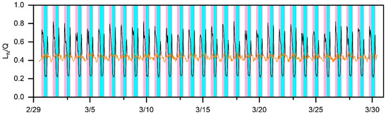
Figure 2.
Temporal changes in from 1 March to 30 March 2020 (UTC). The VOC-sensitive regimes were dominant in the morning and evening (shaded areas in pink) while became more NOx-sensitive in the afternoon (shaded areas in cyan). The black line represents the values of , and the yellow line represents the regime transition threshold.
In this work, the values of γ, [RO2], and [XO2] were obtained from previous studies. To this end, we needed to investigate how these assumptions would affect the identification of the production regimes. We thus conducted sensitivity tests on these three factors. Specifically, the values of γ, [RO2]/[XO2], and [XO2] were altered to 1.0, doubled, and three-fold, respectively (Figure S3). This extended the periods of the NOx-sensitive regime by hours. In contrast, halving the value of [XO2] could shorten the NOx-sensitive regime period. However, we confirmed with the diurnal variation characteristics that became more NOx-sensitive in the afternoon but more VOC-sensitive in the morning, and the evening stayed the same. Collectively, although these variables (i.e., γ, [RO2], and [XO2]) played a key role in altering the duration of the production regime in Chun’an, they would not change the specific production regime.
As shown in Equation (36), there were four terms, i.e., , , , and , that dominated in . Figure 3 shows their explicit the temporal variations. Therein, [NO] presents the largest fluctuations, with an amplitude of two orders of magnitude, while the amplitude of other variables varied by less than one order of magnitude. Figure 4 presents the relationship between and [NO]. It was immediately clear that most of the variations in the former relied on the changes in the latter, especially when the [NO] decreased to less than 0.2 ppb. As illustrated in Figure S4, the periods with the lower [NO] (<0.2 ppb) consistently corresponded to the NOx-sensitive regime. Therefore, our results indicate that, while the transition between the VOC- and NOx-sensitive regimes was related to , , and , the NO depletion played a roughly dominant role in the decreases, and thus, the sensitivity regime transitions during this field campaign.
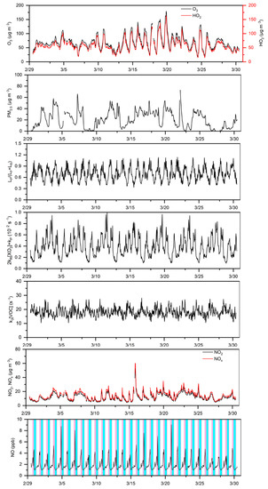
Figure 3.
Temporal variations in key drivers from 1 March to 30 March, 2020 (UTC). These drivers include O3, HO2, k3[VOC], PM2.5, NO2, NOx, LP/(LP+LR), NO, and .
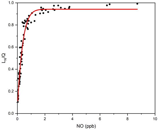
Figure 4.
Relationships between and [NO] during this field campaign. Most of the variations in relied on the changes in [NO], especially when [NO] decreased to less than 0.2 ppb.
Note that as the value of decreased, especially under the regime transition threshold (roughly 0.4) (Figure 2), its uncertainty increased. As such, if [NO] was the key driver, as illustrated above, more reliable [NO] measurements would lead to more accurate classifications of the production regimes. Therefore, not only more NOx emissions from vehicle rush hours in the morning and evening but also more NO depletion from photochemical NOx loss in the afternoon might lead to substantial variations in the [NO], and thus, the sensitivity regime.
Numerous investigations have been conducted to determine the production sensitivities using trace ratios, such as [HCHO]/[NO2] [22,23] and [NMHC]/[NOx] [15,24,25].
Figure 5 illustrates the corresponding classifications of the production regimes for the same period, in which higher ratios represent the NOx-sensitive periods. Previous model studies based on ground-based measurements have shown that P(O3) was absolutely NOx-sensitive at [HCHO]/[NO2] > 1.8, either NOx or VOC-sensitive at [HCHO]/[NO2] = 0.8~1.8, and predominately VOC-sensitive at [HCHO]/[NO2] < 0.8 [22]. In this work, the regime transition threshold was roughly [NMHC]/[NOx] = 14 ppb of C ppb−1, showing slightly lower but fine agreement with that of 20 ppb of C ppb−1 in Tokyo in the summer [15]. It was immediately clear that these regime transitions had a good relationship with our categorization of the production regimes. Such outstanding correlations indirectly confirm that γ, [RO2]/[XO2], and [XO2] had limited impacts on the regime transition, and that the relative sensitivity analysis in this work well captured this transition.
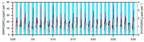
Figure 5.
Temporal changes in [NMHC]/[NOx] and [HCHO]/[NO2] from 1 March to 30 March, 2020 (UTC).
The regime transitions have a good relationship with our categorization of the production regimes in Figure 2. The lines in black and red represent the values of [NMHC]/[NOx] and [HCHO]/[NO2], respectively. The shaded areas in pink and cyan indicate the VOC-sensitive and NOx-sensitive regimes, respectively. Figure 6 presents the daily absolute production sensitivity to precursors (NOx and VOCs) from 22 March to 27 March 2020, in which only daytime absolute sensitivity was analyzed, with positive or negative values. The former indicates that increasing the precursor would result in increases, while the latter indicates that the same situation would lead to the opposite result. As presented in Figure 5a, we found consistently positive values for and negative values for over these dates. This indicates that, throughout this period, VOC and NOx mitigation would decrease and increase , respectively. Moreover, the absolute values on 26 March and 27 March were significantly lower than those on other days. This was mainly due to the changes in meteorological conditions, especially sporadic sprinkling. Another explanation was the wind direction that shifted from southeast to southwest. When an air mass originated from downtown Hangzhou via a southeast wind from 26 March to 27 March, the relatively abundant NOx increased the , while the southwest wind from the rural area from 22 March to 25 March reduced the [NO], and thus, the .
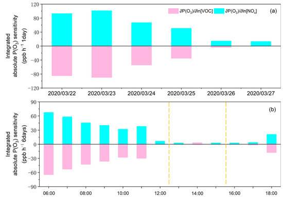
Figure 6.
(a) Day time in each day and (b) 6 days at each time variations in and from 22 March to 27 March 2020 (UTC). Throughout this period, the total absolute sensitivities on NOx were less than those on VOCs. In the afternoon (between the two yellow dashed lines), the absolute sensitivity of NOx might exceed that of VOCs, indicating the NOx-sensitive period.
Figure 6b presents the hourly absolute production sensitivity to precursors (NOx and VOCs) from 26 March to 27 March when a southeast wind blew from downtown Hangzhou. As with the relative sensitivity analysis, in the periods when NOx had a larger absolute sensitivity, the VOCs were categorized as the NOx-sensitive regime periods. Hence, in the afternoon (from 13:00 to 15:00), the absolute sensitivity of NOx exceeded that of the VOCs, indicating the NOx-sensitive regime period. Specifically, the absolute sensitive to both NOx and VOCs was higher in the morning and evening, while it showed a much smaller magnitude in the afternoon. In theory (Equation (4)), relied on both [NO] and . In the afternoon, [NO] was significantly depleted, while [XO2] peaked due to the highest photochemical reaction rates. Yet, the former depletion exceeded the surge in [XO2], thus leading to with a relatively small magnitude. In contrast, the higher [NO] in the morning and evening resulted in an absolute with a large magnitude. Collectively, for the daytime throughout the period, the total absolute sensitivities on NOx were lower than those on VOCs. This suggests that, although was more sensitive to NOx in the afternoon and VOCs in the morning and evening, the total absolute was dominated by the VOC-sensitive regime. As such, the mitigation of VOC emissions (rather than NOx emissions) can play a dominant role in pollution control policies in Chun’an. Note that the magnitude of the absolute sensitivity displayed here was related to the assumed γ, [RO2]/[XO2], and [XO2]. Despite this, the production sensitivity regime would not be changed.
Figure 7 presents the relationship of the total absolute sensitivity during the daytime with the uptake coefficient (γ) over six days (from 22 March to 27 March). Four ensemble sensitivity tests were conducted for the impacts of the potential γ () on the total absolute sensitivity. Therein, 0.2 is the coefficient typically used in model simulations [34] and thus applied in the basic case. By comparison, 0.4 is the maximum value observed in China [35]. γ = 1.0 is the theoretical maximum value at which the impact of uptake is maximal. To this end, 1.0 was treated as the upper boundary.
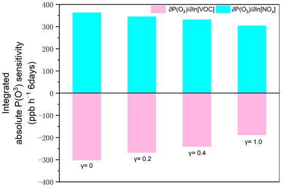
Figure 7.
Impacts of uptake coefficients on the total absolute sensitivity from 22 March to 27 March 2020 (UTC).
In the base case, particle uptakes with γ = 0.2 narrowed the absolute values of positive and negative by 4% and 11%, respectively. This suggests that particle uptakes consistently inhibited not only the impacts of VOC mitigation on the reductions by 4% but also those of NOx reduction on enhancements by 11%. With the increases in γ, such inhibitions were further amplified. If γ = 1.0, the absolute values of and negative were reduced by 16% and 38%.
Subsequently, each total absolute P(O3) sensitivity was normalized by the value with γ = 0. The resulting values were quantitively linked with γ (Figure S5). Consequently, we found that γ increases led to sensitivity decreases, with the highest decline of 30%. In turn, other factors, such as [RO2]/[XO2] and [XO2], would not overturn our detections. Note that PM2.5 concentrations were relatively modest (21 ± 5 μg/m3) throughout this campaign period. In places with a higher PM2.5 concentration, particle uptakes would have bigger impacts on O3 production sensitivity.
4. Conclusions
This work presents a novel observation-based analysis (including relative and absolute analysis) on O3 production sensitivity for a suburban field campaign in Chun’an, where volatile organic compounds (VOCs) and NOx are both rich. The results of the relative sensitivity analysis demonstrate that the dominant precursor for O3 production sensitivity shifts from volatile organic compounds (VOCs) in the morning and evening to NOx in the afternoon, the main driver of which is related to NO depletion. In turn, in view of the absolute sensitivity analysis, we confirm that VOCs persistently determine the diurnal ozone production sensitivity. More importantly, this set of relative and absolute sensitivity analyses prove that particle uptake does not change the regime classification of O3 production sensitivity (i.e., VOC- or NOx-sensitive regime) but potentially has a strong inhibition on the sensitivity magnitude (within 16% and 38% for VOC- or NOx-sensitive regimes, respectively). Our results partly explain more insensitive O3 production measurements than those suggested by traditional sensitivity analyses and have important implications for synergistic controls on O3 and fine particulate matter pollution.
Due to the fact that this field campaign is still limited from the spatiotemporal perspective, it is necessary to continuously promote similar field campaigns with wider coverage and longer duration. Alternatively, numerical chemical transport models or box models might offer valuable source materials for our theoretical analysis [36]. Note that the uncertainties in [XO2] and [RO2]/[XO2] did not affect the qualitative findings in Chun’an, which is possibly not true for other cases. We acknowledge that the quantitative impacts of particle uptake on O3 production remain unclear due to the lack of real-world uptake coefficients. Previous findings have shown that the value of γ ranged between 0.1 and 0.4 [11]. If this range was suitable for our case, the absolute sensitivity had an uncertainty of ±100%. In addition, we set γRO2 to 0 due to the limited references. It is thus necessary to estimate the impacts of γRO2 on the O3 production sensitivity. Looking forward, we can integrate the above relative and absolute sensitivity analysis with observation-constrained chemical transport models. On this basis, we can picture O3 production sensitivity over a large spatiotemporal scale.
Supplementary Materials
The following supporting information can be downloaded at: https://www.mdpi.com/article/10.3390/atmos13101558/s1. Refs. [37,38,39,40,41,42] are cited in Table S1.
Author Contributions
P.L. and L.W. designed this study and wrote the manuscript. L.W. and Y.P. developed the retrieval algorithm. X.C., L.F., X.Z., J.M. and S.C. performed the data analysis. All authors have read and agreed to the published version of the manuscript.
Funding
This study was supported by the National Natural Science Foundation of China (No. 22006030), the Hebei Youth Top Fund (BJ2020032), the Research Foundation of the Education Bureau of Hebei (QN2019184), the Basic Scientific Research Foundation of Hebei (KY2021024), the Initiation Fund of Hebei Agricultural University (412201904 and YJ201833), and the Zhejiang Shuren University Basic Scientific Research Special Funds (2021R020).
Institutional Review Board Statement
Not applicable.
Informed Consent Statement
Not applicable.
Data Availability Statement
The data presented in this study are available on request from the corresponding author. The data are not publicly available due to restrictions apply to the availability of these data, which were used under license for this study.
Acknowledgments
The data were provided by Chun’an Branch of Hangzhou Municipal Ecology and Environment Bureau. The authors are grateful to the reviewers for their meticulous reading of the paper and constructive comments and suggestions.
Conflicts of Interest
The authors declare no conflict of interest.
References
- Monks, P.S.; Archibald, A.T.; Colette, A.; Cooper, O.; Coyle, M.; Derwent, R.; Fowler, D.; Granier, C.; Law, K.S.; Mills, G.E.; et al. Tropospheric ozone and its precursors from the urban to the global scale from air quality to short-lived climate forcer. Atmos. Chem. Phys. 2015, 15, 8889–8973. [Google Scholar] [CrossRef]
- Mills, G.; Buse, A.; Gimeno, B.; Bermejo, V.; Holland, M.; Emberson, L.; Pleijel, H. A synthesis of AOT40-based response functions and critical levels of ozone for agricultural and horticultural crops. Atmos. Environ. 2007, 41, 2630–2643. [Google Scholar] [CrossRef]
- Novak, K.; Skelly, J.M.; Schaub, M.; Kräuchi, N.; Hug, C.; Landolt, W.; Bleuler, P. Ozone air pollution and foliar injury development on native plants of Switzerland. Environ. Pollut. 2003, 125, 41–52. [Google Scholar] [CrossRef]
- Lefohn, A.S.; Malley, C.S.; Smith, L.; Wells, B.; Hazucha, M.; Simon, H.; Naik, V.; Mills, G.; Schultz, M.G.; Paoletti, E. Tropospheric ozone assessment report: Global ozone metrics for climate change, human health, and crop/ecosystem research. Elem. Sci. Anthr. 2018, 6, 27. [Google Scholar] [CrossRef]
- Sun, G.E.; McLaughlin, S.B.; Porter, J.H.; Uddling, J.; Mulholland, P.J.; Adams, M.B.; Pederson, N. Interactive influences of ozone and climate on streamflow of forested watersheds. Glob. Change Biol. 2012, 18, 3395–3409. [Google Scholar] [CrossRef]
- Finlayson-Pitts, B.J.; Pitts, J.N., Jr. Chemistry of the Upper and Lower Atmosphere: Theory, Experiments, and Applications; Elsevier: Amsterdam, The Netherlands, 1999. [Google Scholar]
- Kleinman, L.I.; Daum, P.H.; Lee, J.H.; Lee, Y.-N.; Nunnermacker, L.J.; Springston, S.R.; Newman, L.; Weinstein-Lloyd, J.; Sillman, S. Dependence of ozone production on NO and hydrocarbons in the troposphere. Geophys. Res. Lett. 1997, 24, 2299–2302. [Google Scholar] [CrossRef]
- Kleinman, L.I.; Daum, P.H.; Lee, Y.-N.; Nunnermacker, L.J.; Springston, S.R.; Weinstein-Lloyd, J.; Rudolph, J. Sensitivity of ozone production rate to ozone precursors. Geophys. Res. Lett. 2001, 28, 2903–2906. [Google Scholar] [CrossRef]
- Kleinman, L.I. The dependence of tropospheric ozone production rate on ozone precursors. Atmos. Environ. 2005, 39, 575–586. [Google Scholar] [CrossRef]
- Kleinman, L.I. Ozone process insights from field experiments—Part II: Observation-based analysis for ozone production. Atmos. Environ. 2000, 34, 2023–2033. [Google Scholar] [CrossRef]
- Taketani, F.; Kanaya, Y.; Pochanart, P.; Liu, Y.; Li, J.; Okuzawa, K.; Kawamura, K.; Wang, Z.; Akimoto, H. Measurement of overall uptake coefficients for HO2 radicals by aerosol particles sampled from ambient air at Mts. Tai and Mang (China). Atmos. Chem. Phys. 2012, 12, 11907–11916. [Google Scholar] [CrossRef]
- George, I.; Matthews, P.; Whalley, L.; Brooks, B.; Goddard, A.; Baeza-Romero, M.; Heard, D. Measurements of uptake coefficients for heterogeneous loss of HO2 onto submicron inorganic salt aerosols. Phys. Chem. Chem. Phys. 2013, 15, 12829–12845. [Google Scholar] [CrossRef] [PubMed]
- Zou, Q.; Song, H.; Tang, M.; Lu, K. Measurements of HO2 uptake coefficient on aqueous (NH4)2SO4 aerosol using aerosol flow tube with LIF system. Chin. Chem. Lett. 2019, 30, 2236–2240. [Google Scholar] [CrossRef]
- Ammann, M.; Cox, R.A.; Crowley, J.N.; Jenkin, M.E.; Mellouki, A.; Rossi, M.J.; Troe, J.; Wallington, T.J. Evaluated kinetic and photochemical data for atmospheric chemistry: Volume VI—Heterogeneous reactions with liquid substrates. Atmos. Chem. Phys. 2013, 13, 8045–8228. [Google Scholar] [CrossRef]
- Kanaya, Y.; Fukuda, M.; Akimoto, H.; Takegawa, N.; Komazaki, Y.; Yokouchi, Y.; Koike, M.; Kondo, Y. Urban photochemistry in central Tokyo: Rates and regimes of oxidant (O3+ NO2) production. J. Geophys. Res. 2008, 113, 8671. [Google Scholar] [CrossRef]
- Xie, M.; Zhu, K.; Wang, T.; Chen, P.; Han, Y.; Li, S.; Zhuang, B.; Shu, L. Temporal characterization and regional contribution to O3 and NOx at an urban and a suburban site in Nanjing, China. Sci. Total Environ. 2016, 551–552, 533–545. [Google Scholar] [CrossRef] [PubMed]
- Ye, Q.; Krechmer, J.E.; Shutter, J.D.; Barber, V.P.; Li, Y.; Helstrom, E.; Franco, L.J.; Cox, J.L.; Hrdina, A.I.H.; Goss, M.B.; et al. Real-Time Laboratory Measurements of VOC Emissions, Removal Rates, and Byproduct Formation from Consumer-Grade Oxidation-Based Air Cleaners. Environ. Sci. Technol. Lett. 2021, 8, 1020–1025. [Google Scholar] [CrossRef]
- Kaser, L.; Peron, A.; Graus, M.; Striednig, M.; Wohlfahrt, G.; Juráň, S.; Karl, T. Interannual variability of terpenoid emissions in an alpine city. Atmos. Chem. Phys. 2022, 22, 5603–5618. [Google Scholar] [CrossRef]
- Hammer, M.U. Findings on H2O2/HNO3 as an indicator of ozone sensitivity in Baden-Württemberg, Berlin-Brandenburg, and the Po valley based on numerical simulations. J. Geophys. Res. 2002, 107, 211. [Google Scholar]
- Peng, Y.P.; Chen, K.S.; Lai, C.H.; Lu, P.J.; Kao, J.H. Concentrations of H2O2 and HNO3 and O3–VOC–NOx sensitivity in ambient air in southern Taiwan. Atmos. Environ. 2006, 40, 6741–6751. [Google Scholar] [CrossRef]
- Sillman, S.; He, D.; Pippin, M.R.; Daum, P.H.; Imre, D.G.; Kleinman, L.I.; Lee, J.H.; Weinstein-Lloyd, J. Model correlations for ozone, reactive nitrogen, and peroxides for Nashville in comparison with measurements: Implications for O3-NOx-hydrocarbon chemistry. J. Geophys. Res. Atmos. 1998, 103, 22629–22644. [Google Scholar] [CrossRef]
- Tonnesen, G.S.; Dennis, R.L. Analysis of radical propagation efficiency to assess ozone sensitivity to hydrocarbons and NOx: Local indicators of instantaneous odd oxygen production sensitivity. J. Geophys. Res. Atmos. 2000, 105, 9213–9225. [Google Scholar] [CrossRef]
- Sillman, S.; He, D.; Cardelino, C.; Imhoff, R.E. The Use of Photochemical Indicators to Evaluate Ozone-NOx-Hydrocarbon Sensitivity: Case Studies from Atlanta, New York, and Los Angeles. J. Air Waste Manag. Assoc. 1997, 47, 1030–1040. [Google Scholar] [CrossRef]
- Kanaya, Y.; Pochanart, P.; Liu, Y.; Li, J.; Tanimoto, H.; Kato, S.; Suthawaree, J.; Inomata, S.; Taketani, F.; Okuzawa, K. Rates and regimes of photochemical ozone production over Central East China in June 2006: A box model analysis using comprehensive measurements of ozone precursors. Atmos. Chem. Phys. 2009, 9, 7711–7723. [Google Scholar] [CrossRef]
- Sillman, S. The relation between ozone, NOx and hydrocarbons in urban and polluted rural environments. Atmos. Environ. 1999, 33, 1821–1845. [Google Scholar] [CrossRef]
- Sakamoto, Y.; Sadanaga, Y.; Li, J.; Matsuoka, K.; Takemura, M.; Fujii, T.; Nakagawa, M.; Kohno, N.; Nakashima, Y.; Sato, K.; et al. Relative and Absolute Sensitivity Analysis on Ozone Production in Tsukuba, a City in Japan. Environ. Sci. Technol. 2019, 53, 13629–13635. [Google Scholar] [CrossRef]
- Pöschl, U.; Rudich, Y.; Ammann, M. Kinetic model framework for aerosol and cloud surface chemistry and gas-particle interactions—Part 1: General equations, parameters, and terminology. Atmos. Chem. Phys. 2007, 7, 5989–6023. [Google Scholar] [CrossRef]
- Fuchs, N.; Sutugin, A.G. High-dispersed aerosols. In Topics in Current Aerosol Research; Elsevier: Amsterdam, The Netherlands, 1971; p. 1. [Google Scholar]
- Sadanaga, Y. The importance of NO2 and volatile organic compounds in the urban air from the viewpoint of the OH reactivity. Geophys. Res. Lett. 2004, 31. [Google Scholar] [CrossRef]
- Sadanaga, Y.; Yoshino, A.; Watanabe, K.; Yoshioka, A.; Wakazono, Y.; Kanaya, Y.; Kajii, Y. Development of a measurement system of OH reactivity in the atmosphere by using a laser-induced pump and probe technique. Rev. Sci. Instrum. 2004, 75, 2648–2655. [Google Scholar] [CrossRef]
- Sadanaga, Y.; Yoshino, A.; Kato, S.; Kajii, Y. Measurements of OH reactivity and photochemical ozone production in the urban atmosphere. Environ. Sci. Technol. 2005, 39, 8847–8852. [Google Scholar] [CrossRef] [PubMed]
- Griffith, S.M.; Hansen, R.F.; Dusanter, S.; Michoud, V.; Gilman, J.B.; Kuster, W.C.; Veres, P.R.; Graus, M.; Gouw, J.A.; Roberts, J.; et al. Measurements of hydroxyl and hydroperoxy radicals during CalNex-LA: Model comparisons and radical budgets. J. Geophys. Res. Atmos. 2016, 121, 4211–4232. [Google Scholar] [CrossRef]
- Lou, S.; Holland, F.; Rohrer, F.; Lu, K.; Bohn, B.; Brauers, T.; Chang, C.C.; Fuchs, H.; Häseler, R.; Kita, K.; et al. Atmospheric OH reactivities in the Pearl River Delta–China in summer 2006: Measurement and model results. Atmos. Chem. Phys. 2010, 10, 11243–11260. [Google Scholar] [CrossRef]
- Stadtler, S.; Simpson, D.; Schröder, S.; Taraborrelli, D.; Bott, A.; Schultz, M. Ozone impacts of gas–aerosol uptake in global chemistry transport models. Atmos. Chem. Phys. 2018, 18, 3147–3171. [Google Scholar] [CrossRef]
- Yoshino, A.; Sadanaga, Y.; Watanabe, K.; Kato, S.; Miyakawa, Y.; Matsumoto, J.; Kajii, Y. Measurement of total OH reactivity by laser-induced pump and probe technique—comprehensive observations in the urban atmosphere of Tokyo. Atmos. Environ. 2006, 40, 7869–7881. [Google Scholar] [CrossRef]
- Mazzuca, G.M.; Ren, X.; Loughner, C.P.; Estes, M.; Crawford, J.H.; Pickering, K.E.; Weinheimer, A.J.; Dickerson, R.R. Ozone production and its sensitivity to NO2 and VOCs: Results from the DISCOVER-AQ field experiment, Houston. Atmos. Chem. Phys. 2016, 16, 14463–14474. [Google Scholar] [CrossRef]
- Burkholder, J.; Sander, S.; Abbatt, J.; Barker, J.; Cappa, C.; Crounse, J.; Dibble, T.; Huie, R.; Kolb, C.; Kurylo, M. Chemical Kinetics and Photochemical Data for Use in Atmospheric Studies; Evaluation Number 19; Jet Propulsion Laboratory, National Aeronautics and Space: Pasadena, CA, USA, 2020. [Google Scholar]
- Atkinson, R.; Baulch, D.; Cox, R.; Hampson, R., Jr.; Kerr, J.; Rossi, M.; Troe, J. Evaluated kinetic and photochemical data for atmospheric chemistry, organic species: Supplement VII. J. Phys. Chem. Ref. Data 1999, 28, 191–393. [Google Scholar] [CrossRef]
- Kanno, N.; Tonokura, K.; Koshi, M. Equilibrium constant of the HO2-H2O complex formation and kinetics of HO2 + HO2-H2O: Implications for tropospheric chemistry. J. Geophys. Res. Atmos. 2006, 111, D20. [Google Scholar] [CrossRef]
- Saunders, S.M.; Jenkin, M.E.; Derwent, R.; Pilling, M. Protocol for the development of the Master Chemical Mechanism, MCM v3 (Part A): Tropospheric degradation of non-aromatic volatile organic compounds. Atmos. Chem. Phys. 2003, 3, 161–180. [Google Scholar] [CrossRef]
- Sadanaga, Y.; Kondo, S.; Hashimoto, K.; Kajii, Y. Measurement of the rate coefficient for the OH+ NO2 reaction under the atmospheric pressure: Its humidity dependence. Chem. Phys. Lett. 2006, 419, 474–478. [Google Scholar] [CrossRef]
- Kanaya, Y.; Cao, R.; Akimoto, H.; Fukuda, M.; Komazaki, Y.; Yokouchi, Y.; Koike, M.; Tanimoto, H.; Takegawa, N.; Kondo, Y. Urban photochemistry in central Tokyo: 1. Observed and modeled OH and HO2 radical concentrations during the winter and summer of 2004. J. Geophys. Res. Atmos. 2007, 112, D21. [Google Scholar] [CrossRef]
Publisher’s Note: MDPI stays neutral with regard to jurisdictional claims in published maps and institutional affiliations. |
© 2022 by the authors. Licensee MDPI, Basel, Switzerland. This article is an open access article distributed under the terms and conditions of the Creative Commons Attribution (CC BY) license (https://creativecommons.org/licenses/by/4.0/).