Article

Daily River Water Temperature Prediction: A Comparison between Neural Network and Stochastic Techniques

1
Department of Hydrology and Water Management, Institute of Physical Geography and Environmental Planning, Adam Mickiewicz University, 61-680 Poznań, Poland
2
Department of Water Engineering, Faculty of Agriculture, Bu-Ali Sina University, Hamedan 65178-38695, Iran
*
Author to whom correspondence should be addressed.
Atmosphere 2021, 12(9), 1154; https://doi.org/10.3390/atmos12091154
Submission received: 7 August 2021 / Revised: 4 September 2021 / Accepted: 5 September 2021 / Published: 7 September 2021
(This article belongs to the Special Issue River Water Temperature and Ice Phenomena Modeling and Forecasting)

Abstract

:
The temperature of river water (TRW) is an important factor in river ecosystem predictions. This study aims to compare two different types of numerical model for predicting daily TRW in the Warta River basin in Poland. The implemented models were of the stochastic type—Autoregressive (AR), Moving Average (MA), Autoregressive Moving Average (ARMA) and Autoregressive Integrated Moving Average (ARIMA)—and the artificial intelligence (AI) type—Adaptive Neuro Fuzzy Inference System (ANFIS), Radial Basis Function (RBF) and Group Method of Data Handling (GMDH). The ANFIS and RBF models had the most fitted outputs and the AR, ARMA and ARIMA patterns were the most accurate ones. The results showed that both of the model types can significantly present suitable predictions. The stochastic models have somewhat less error with respect to both the highest and lowest TRW deciles than the AIs and were found to be better for prediction studies, with the GMDH complex model in some cases reaching Root Mean Square Error (RMSE) = 0.619 °C and Nash-Sutcliff coefficient (NS) = 0.992, while the AR(2) simple linear model with just two inputs was partially able to achieve better results (RMSE = 0.606 °C and NS = 0.994). Due to these promising outcomes, it is suggested that this work be extended to other catchment areas to extend and generalize the results.

1. Introduction

For the monitoring of ecological status and proper functioning of the water ecosystem, it is important to have information about a river’s thermal conditions [1]. The TRW is a good indicator of the control of hydrological and environmental pollution processes in water ecosystems [2].
Due to the influence of many factors which shape the features of the thermal regime of waters, predictions of changes and forecasts of TRW are a complex process [3]. Predictive and prognostic models of TRW changes take into account relationships with meteorological and hydrological factors, as well as morphological parameters [4,5,6,7]. Brosofske et al. [8], conducting research in western Washington, showed that significant changes in the reference characteristics of RWT are also caused by the features of the microclimate in the riparian zones of streams, which are often transformed by various forms of anthropogenic activity. In their opinion, a buffer 45 m wide (on each side of the stream) is necessary to maintain a natural riparian microclimatic environment along the streams. Air temperature is an important predictor of changes in TRW, and its relationships have been confirmed taking into account the nature of short-term to long-term fluctuations [9,10,11,12]. In TRW prediction, regression models and artificial intelligence models (AIs) are most often based on air temperature data [13,14,15,16,17,18,19]. Zhu and Piotrowski [3] presented a comprehensive review of research and methods for forecasting TRW using AI models. The high efficiency of artificial neural networks in TRW forecasting has been confirmed in various regions [20,21,22,23].
Many studies show that Multi-Layer Perceptron (MLP) and ANFIS models are gaining importance in hydrological applications [24,25,26,27]. In TRW modeling, the most commonly used type of artificial neural network (ANN) is the so-called multilayer perceptron neural network (MLPNN). Daigle et al. [28] used MLPNNs to estimate the start date of the seasonal temperature cycle in various streams located in Canada and the northern United States, and demonstrated that they compare favorably with simple regression methods. Faruk [29] combined MLPNNs with ARIMA models for autoregressive jet temperature modeling, while Tao et al. [30] used MLPNNs for autoregressive stream water temperature modeling with exogenous inputs. Additionally, hybrid models are used that combine wavelet transform (WT) and Ais, e.g., WTMLP (WTMLPNN), which, however, have not been widely used in forecasting the TRW. Hybrid WT-ANN models have been used by [22,31,32]. The neural network model types, such as the Radial Basis Function (RBF) or Group Method of Data Handling (GMDH), are rarely used to predict hydrological variables, especially in TRW forecasting research. They are, however, already used in many other areas of data mining for prognosis and modeling, as well as optimization and data pattern recognition.
The literature describes the use of stochastic models to simulate and forecast the daily stream water temperature. In stochastic models, the TRW is modeled as a function of time consisting of two different components: a short- and a long-term component [33,34]. These models typically use water temperature lag, residual air temperature and flow rates as exogenous variables. Stochastic models that take into account the relationship between TRW and air temperature have been successfully developed in Canadian rivers, e.g., in the Catamaran Brook stream in New Brunswick [33] and in the Moisie River [35], in the Drava River in Croatia [36,37], the Missouri River in the USA [34], and in Poland the Noteć River [11]. Various stochastic approaches are used to model residual TRW representing short-term fluctuations, e.g., multiple regression, the second-order autoregressive model, and the Box and Jenkins model [35]. In the present case, the second-order autoregressive model gave the best results. The TRW model in the Box–Jenkins time series was successfully applied by Benyahya et al. [38], who conducted a comparison of non-parametric and parametric models of Nivelle River in France.
The time series model has been widely used as a statistical model in hydrological and meteorological prediction studies [39,40,41,42]. The assumptions of these types of models were developed by Box and Jenkins [43] within the general concept of stochastic hydrological models, as some of the most effective methods of forecasting. The ARIMA model has the advantages of fast modeling and prediction, and also uses only the time lags of the target variable as inputs [44]. For example, in forecasting TRW, ARIMA uses just the time lags of TRW itself and does not need other hydro-meteorological variables, such as air temperature, flow discharge, etc. The ARIMA model is widely used in the prediction of time series data: discharge patterns [45,46,47,48,49,50,51], river water characteristics [52,53,54], and water consumption [55,56]. However, in the literature, there are few studies that use Box–Jenkins stochastic models for forecasting TRW time series.
Most TRW prediction models use meteorological variables, mainly air temperature, as input for the models. Similarly, artificial intelligence models are most often based on air temperature data. The most common are MLP, ANFIS and WTMLP, while the RBF and GMDH models have not been used for this purpose.
The aim of the article is to present the results of research into the use of stochastic models and artificial intelligence (AI) in TRW predictions. We predicted the daily TRW using only the time lags of the variable itself. Other parameters (e.g., hydrological or meteorological) were not taken into account. With respect to the current research, we present a new investigation in the field of TRW testing, consisting of the application, in addition to the commonly used ANFIS from the AI group, of the RBF and GMDH models. Another novelty of our study consists in the comparison of the results of the stochastic models with the AI models in terms of their performance by applying evaluation measurements and indicating the most accurate prediction models.

2. Methodology

2.1. Study Area and Source Material

The TRW modeling was carried out for the Warta River (Figure 1), the third longest river in Poland (length = 808.2 km). The Warta River is a tributary of the Odra River that carries water from the western part of Poland to the Baltic Sea. The basin area is characterized by its considerable size (54,529 km2), and also by the large variety of environmental conditions. The sources of the river are located at an altitude of 380 m above sea level, while it flows into the Odra at an altitude of 12 m above sea level. From the middle section the Warta River is a Ist and IInd shipping class waterway, while in the metropolitan area (21 municipalities including Poznań) it flows through a water intake protection zone (Mosina-Krajkowo Intake), which supplies a large part of the metropolitan population with drinking water. On the river, just below Sieradz, is the Jeziorsko Reservoir, with an area of 42.3 km2 and a dam in Skęczniew, which was built mainly to protect against floods. The Warta River is of great ecological importance, being a habitat for many species of fish and other organisms for which TRW is an important abiotic factor, shaping the conditions of their existence and evolution. It flows through lands of high natural value, including protected areas such as the Wielkopolski National Park (middle course) and the Warta Estuary National Park (lower course), and many locations of importance for the protection of habitats and birds, which were created under the European Natura 2000 project.
Due to the large latitudinal and longitudinal extent of the Warta River catchment area, regional differences in climatic conditions are visible within its range. The area belongs to nine climatic regions [57]. The average annual temperature in the river basin ranges from 7.5 °C in the north to 8.5 °C in the west. Annual precipitation totals range from 520 mm in the northeast to 675 mm in the south.
In Poland, TRW measurements are conducted using the standard measurement and observation network of the Institute of Meteorology and Water Management—National Research Institute (IMWM-NRI, Warsaw, Poland). Measurements are performed daily at 7:00 a.m. (GMT + 1) at water gauge stations using automatic station probes. Research made use of daily TRW values for four gauge stations located on the Warta River (Figure 1, Table 1): Bobry, Sieradz, Poznań and Gorzow Wielkopolski. The data were obtained from the database of the IMWM-NRI and covered a period of 20 hydrological years (1990–2009, specifically from 1 November 1989 to 31 October 2009).

2.2. Stochastic Models (Time Series Model)

A time series model is commonly used to simulate the data sorted by time. The time series of TRW can be considered as the result of a stochastic process. In this study, Autoregressive (AR), Moving Average (MA), Autoregressive Moving Average (ARMA) and Autoregressive Integrated Moving Average (ARIMA) time series models were used for TRW modeling. The ARMA and ARIMA models combine two basic models: the autoregressive and the moving-average. The construction of models is based on the autocorrelation phenomenon, i.e., on the correlation of the value of the forecasting variable with the time lags of the same variable [43].
The AR model is based on the assumption that there is an autocorrelation between the values of the predictable variable (target variable) and its values lagged in time. The form of the AR model is as follows:
y t = φ 0 + φ 1 y t 1 + φ 2 y t 2 + + φ p y t p + e t
where { y t , y t 1 , y t 2 ,…, y t p } are the values of the predictable variable at the time steps { t ,   t 1 , t 2 ,…, t p }, respectively, { φ 0 , φ 1 , φ 2 ,…, φ p } are the model parameters, e t is model error (remainder) for time t , p is the amount of the time lag. The AR model is shown by its autoregressive degree (p) as AR(p).
The MA model expresses the value of the variable as a function of the delayed values of the (stationary) random component. The equation form of MA model is as follows:
y t = θ 0 + e t θ 1 e t 1 θ 2 e t 2 θ q e t q
where y t is the value of the target variable predicted in time t , { e t , e t 1 , e t 2 ,…, e t q } are errors (residuals) of the model at times { t ,   t 1 , t 2 ,…, t q }, { θ 0 , θ 1 , θ 2 ,…, θ q } are the model parameters, and q is the amount of the time lag. The model is assigned moving average degree (q) as MA (q).
Combining the autoregressive and moving average model leads to ARMA, while adding the Integrated component to this model gives the ARIMA model; these have been shown below as equations [58]:
y t = φ 1 y t 1 + φ 2 y t 2 + + φ p y t p + e t + θ 0 θ 1 + e t 1 θ 2 e t 2 θ q e t q
y t = φ 1 y t 1 + φ 2 y t 2 + + φ p y t p + e t + θ 0 θ 1 + e t 1 θ 2 e t 2 θ q e t q y t d
where d is the differencing degree, which is related to the Integrated component. This ARMA is shown by its AR and MA degrees (p and q) as ARMA(p,q), while ARIMA additionally has an Integrated degree (d), making it ARIMA(p,d,q).

2.3. Artificial Intelligence Models

In this study, use was made of the Adaptive Neuro–Fuzzy Inference System (ANFIS), the Radial Basis Function (RBF) neural network, and the Group Method of Data Handling (GMDH) from the Artificial Intelligence models group.

2.3.1. Adaptive Neuro–Fuzzy Inference System (ANFIS)

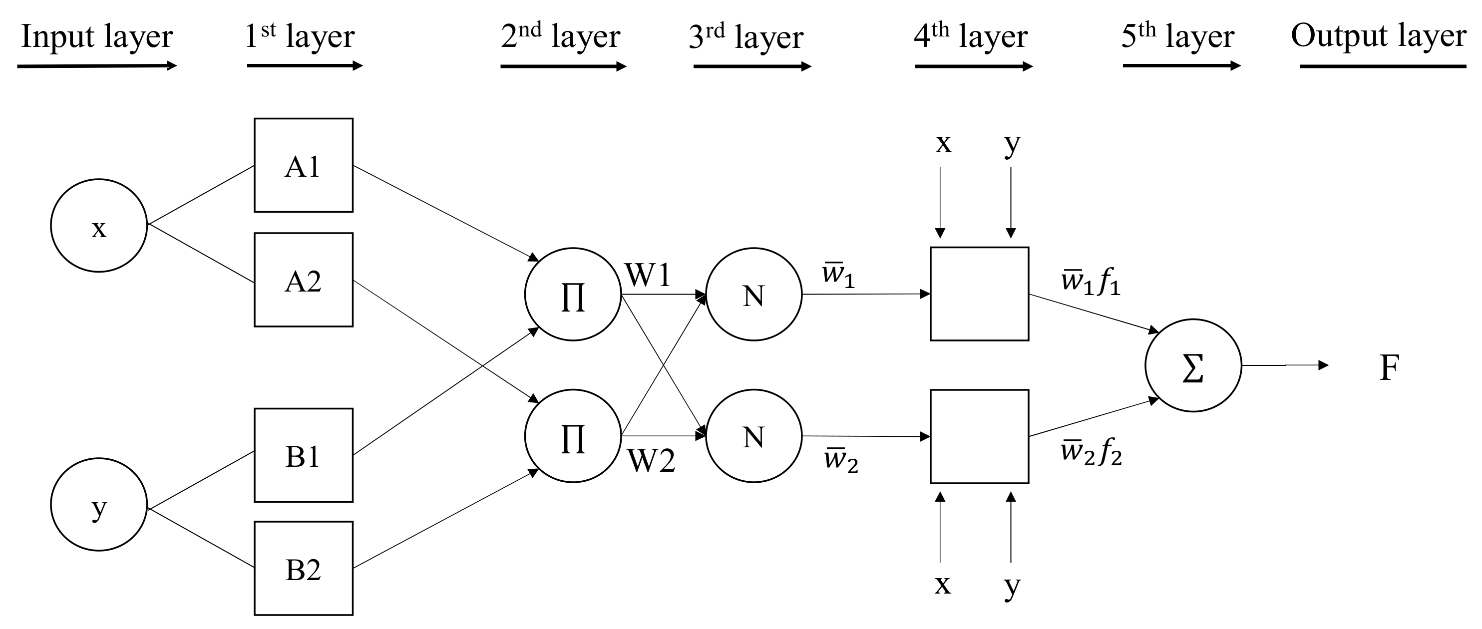
The Adaptive Neuro–Fuzzy Inference System (ANFIS) is used primarily in automation and robotics related to control, decision making, and in the monitoring and diagnostics of hardly measurable processes and parameters. Uncertainty modeling is performed using the description of fuzzy variables based on so-called fuzzy logic. ANFIS is an alternative to systems based on models and traditional numerical algorithms in situations where information about a given field is uncertain and ambiguously formalized [59]. The system is a kind of artificial neural network (ANN) based on the fuzzy inference system (FIS). As part of this model, FIS provides an inference scheme, i.e., a method of constructing logical rules that are learned according to an algorithm taken from the theory of neural networks [60,61]. The learning rule of ANFIS, which determines its parameters, is a combination of methods, back-propagation, and least squares [62,63]. Inference in the neural-fuzzy system proceeds according to specific stages, each of which is carried out by an appropriate layer of the neural structure or similar. The first layer of the structure recreates the membership functions of fuzzy sets included in the premises of the rules. The second layer performs the operations of intersecting fuzzy sets using the algebraic product. The third and fourth layers perform operations related to sharpening the resulting membership function.
A linear combination of the consequent parameters is the result of the ANFIS model. The final output f o u t can be written as [64]:
c f o u t = ω ¯ 1 f 1 + ω ¯ 2 f 2 = ω 1 ω 1 + ω 2 f 1 + ω 2 ω 1 + ω 2 f 2 = ω ¯ 1 x p 1 + ω ¯ 1 y q 1 + ω ¯ 1 r 1 + ω ¯ 2 x p 2 + ω ¯ 2 y q 2 + ω ¯ 2 r 2
where ω i (output) represents the firing strength of a rule, f 1 and f 2 are the fuzzy rules, x and y are the input nodes of ANFIS, and p i , q i and r i are the parameters set (consequent parameters).
The FIS usually uses two methods of inference: The Mamdani method [65] and the Sugeno method [66]. In the present modeling, the latter method was employed. Figure 2 shows a schematic diagram of ANFIS modeling processes.

2.3.2. Radial Basis Function (RBFNN) Neural Network

Radial Basis Functions (RBF) are used in approximation functions for timing and control sequences. In artificial neural networks, radial basis functions are used as activation functions. Neural networks with radial basis functions have found application in solving classification problems, approximating tasks of multivariable functions, and in prediction problems [67,68,69,70].
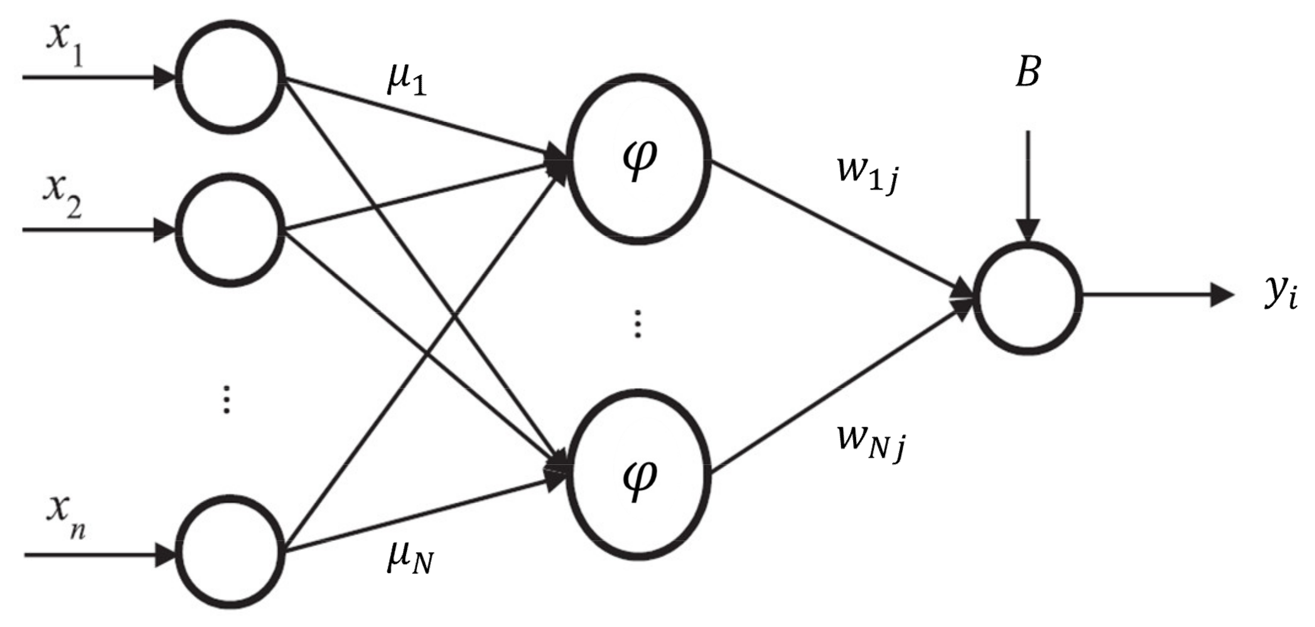
The idea of the RBF network is based on the solutions of statistical methods of approximating the function of a numeric variable. A typical RBNFN is a structure containing: an input layer on which signals described by the input vector x are applied, a hidden layer with radial neurons (weights correspond to cluster center, usually the Gaussian function), and an output layer normally composed of one neuron (linear weighted sum), whose role is the weight summation of signals from hidden neurons [71]. Figure 3 presents the topology of the RBF model as a multi-input–single-output network composition.
The RBFNN Gaussian function ( φ ) takes the form of:
φ x = e x p x μ i 2   2 σ i 2   i = 1 ,   2 ,   N  
where σ is the widths (or spread) of the hidden neuron.
The output layer ( y i ) in RBF can be written as:
y i = j = 1 N w i j   φ j x + B
where w i j   represents a weighted connection between the radial basis function neuron and output neuron; and N is the number of hidden-layer neurons. The constant term B represents a bias.

2.3.3. Group Method of Data Handling (GMDH) Neural Network

The GMDH network is a fast-learning machine based on the principle of heuristic self-organization [72,73]. It is a polynomial theory of complex systems that is applied in a wide variety of areas in data mining and knowledge discovery, forecasting and systems modeling, and optimization and pattern recognition [74].
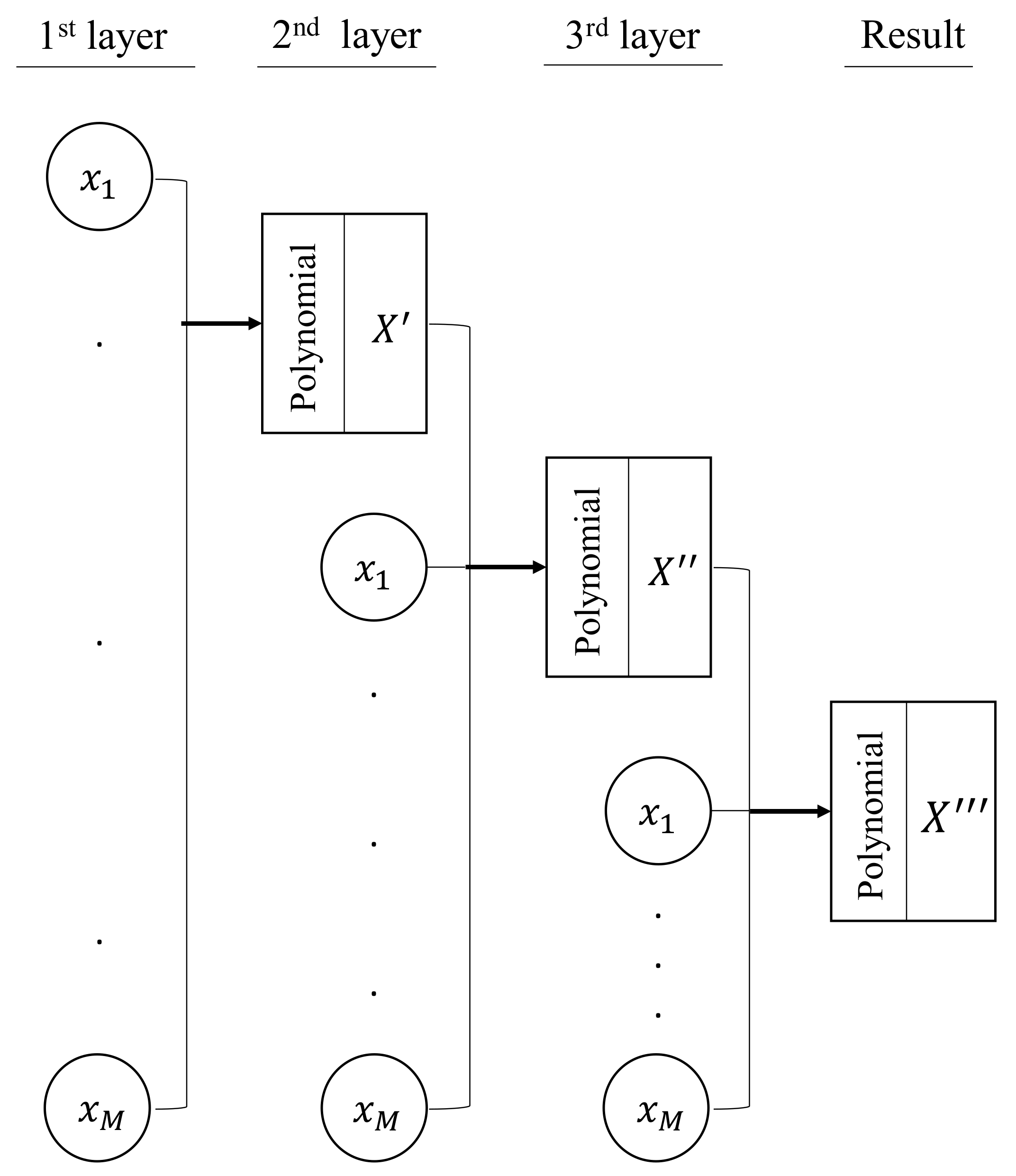
The Group Method of Data Handling (GMDH) is a self-organizing methodology, with the choice of input variables being made automatically. This is a combinatorial multi-layer algorithm in which a network of layers and nodes is generated using several inputs from the data stream being evaluated. The architecture of a polynomial network is formed during the training process, and the node activation function is based on elementary polynomials of arbitrary order [75,76].
A model which uses the GMDH algorithm creates a network of neurons. Through the connections par neurons via of quadratic and triquadratic polynomials, in each layer, new neurons are spawned. The formal assumption is to find a function, f ^ , that can be approximately used instead of an actual function, f , in order to predict the output, y ^ , for a given input vector, X = x 1 ,   x 2 ,   x 3 , x n , as close as possible to its actual output, y [74].
In this case:
y i = f   x i 1 ,   x i 2 ,   x i 3 , x i n ;   i = 1 ,   2 ,     , M
It is now possible to train a GMDH network to predict the output values, y i ^ , for any given input vector, X = x i 1 ,   x i 2 ,   x i 3 , x i n :
y i ^ = f ^ x i 1 ,   x i 2 ,   x i 3 , x i n ;   i = 1 ,   2 ,     , M
To minimize the square of the difference between actual and predicted output, it is necessary to determine a GMDH network, that is:
i = 1 M f ^ x i 1 ,   x i 2 ,   x i 3 , x i n y i 2 min
A connection between inputs and outputs can be expressed by the series functions of Volterra, which is the discrete analogous of the polynomial of Kolmogorov-Gabor [77,78].
y = a + 1 = 1 m b i   x i + i = 1 m j = 1 m c i j x i x j + i = 1 m j = 1 m k = 1 m d i j k x i x j x k +
where {x1, x2, x3 …}: inputs; {a, b, c …}: polynomial coefficients; and y: the node output. Figure 4 shows a schematic diagram of a GMDH model with three layers and M numbers of input variables.

2.4. Evaluation Criteria

Several evaluation criteria were used to assess the accuracy of the modeling process and evaluate the correlation between observed-predicted samples: Root Mean Square Error (RMSE), Normalized Root Mean Square Error (NRMSE), Mean Absolute Error (MAE), coefficient of determination R2, and the Nash–Sutcliffe efficiency criterion (NS). The RMSE and MAE show the difference between predictions and actual values, while the NRMSE is a non-dimensional form of the RMSE. The R2 criterion is used to evaluate the correlation between predictions and actual values. The Nash–Sutcliffe efficiency criterion (NS) normalizes the variance of the errors with the variance of the measurements [79]. These criteria are defined by the following equations:
RMSE = 1 n i = 1 n y i f i 2
NRMSE = 1 n i = 1 n y i f i 2 y m a x y m i n
MAE = 1 n i = 1 n y i f i
R 2 = i = 1 N y i y ¯ ( f i f ) ¯ i = 1 N ( y i y ) ¯ 2 * i = 1 N ( f i f ) ¯ 2 2
NS = 1 i = 1 n y i f i 2 i = 1 n y i y ¯ 2
where y i and y ¯ —observed data and mean of the observed data (respectively); f i and f ¯ —forecast data and mean of the forecast data (respectively); n —number of forecast data; and y m a x and y m i n —extreme values. When the RMSE, MAE and NRMSE are closer to zero, and R2 and NS are approaching 1, then the performance of the models is more favorable. When an NRMSE value is greater than 0.3 then the model is poor. High performance is achieved with values below 0.1 [50].
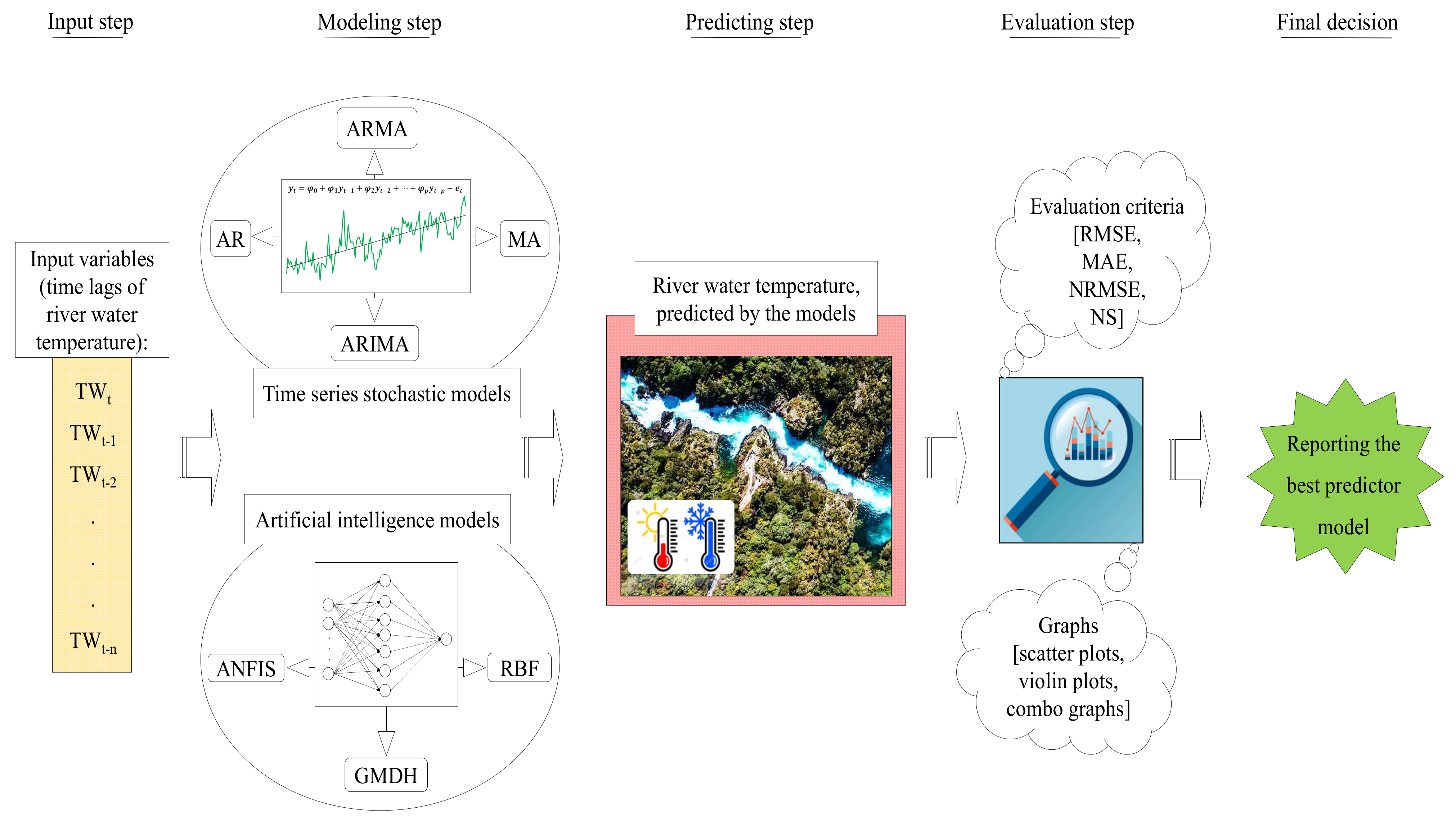
The general process of modeling and predicting the time series of TRW is shown as a flowchart in Figure 5.
In the current study, Minitab software was used for time series analysis and the implementation of stochastic models (AR, MA, ARMA and ARIMA), while MATLAB software was employed to implement the machine learning models (ANFIS, RBF and GMDH). Graphs of the results were prepared using Minitab, Excel and R software.

3. Results

3.1. Modeling and Predicting TRW

To predict TRW, an input variable was determined in an initial step. To make a reasonable comparison between several models, they must use the same input variables. As the stochastic models can only use the main variable’s previous amounts (time lags) as inputs, it is logical to use the time lags of TW for neural network models too. In this study, therefore, the daily time lags of TRW for each hydrometric station were investigated through Autocorrelation (ACF) and Partial Autocorrelation (PACF) functions. The graphs of these two functions are presented in Figure 6.
The ACF and PACF graphs are drawn for time lags of 130 days (Figure 6). ACF plots for all stations indicate that there is no seasonal degree in the daily TRW time series, and we must therefore use non-seasonal patterns for the stochastic models. Furthermore, the ACFs show a decreasing trend of correlation as time lags increase. The autocorrelations are significant for daily time lags up to the 77th day, but using all of them as inputs increases model complexity and violates the principle of parsimony [57]. Finally, when correlations decrease, usage of the less correlated lags increases the prediction error. Thus, it is better to use the most correlated time lags. In these ACF graphs, the time lags 1, 2, 3, 4 and 5 have the largest correlation amounts and have therefore been selected as input variables. In the PACF graphs, too, there are some significantly correlated time lags, i.e., the time lags of 1, 2, 3, 4, 5, 6, 7 and 8 days for the Bobry station, of 1, 2, 3, 4 and 5 days for the Sieradz station, of 1, 2 and 3 days for the Poznań station, and of 1, 2 and 3 days for the Gorzow Wielkopolski station. However, among them, the one-day time lag is specifically the most correlated, so the PACF graphs only suggest the 1st time lag of TRW as their predictor input.
After preparing the input-target samples, the data are divided into two parts of training and testing (as per Table 1). The best stochastic models are identified by trial and error of the Autoregressive, Moving Average and Integrated degrees, up to five non-seasonal degrees. This includes five models for the patterns AR and MA, 25 models for ARMA, and 125 models for ARIMA. The artificial intelligence models were each optimized by the trial and error of their own parameters: the ANFIS model was developed based on the fuzzy c-means (FCM) clustering method, with its optimization parameter being the number of clusters; the RBF’s parameters are the spread and the maximum neurons; and the GMDH’s parameters are the number of layers and the number of neurons in each layer. The modeling and prediction results are shown in Table 2.
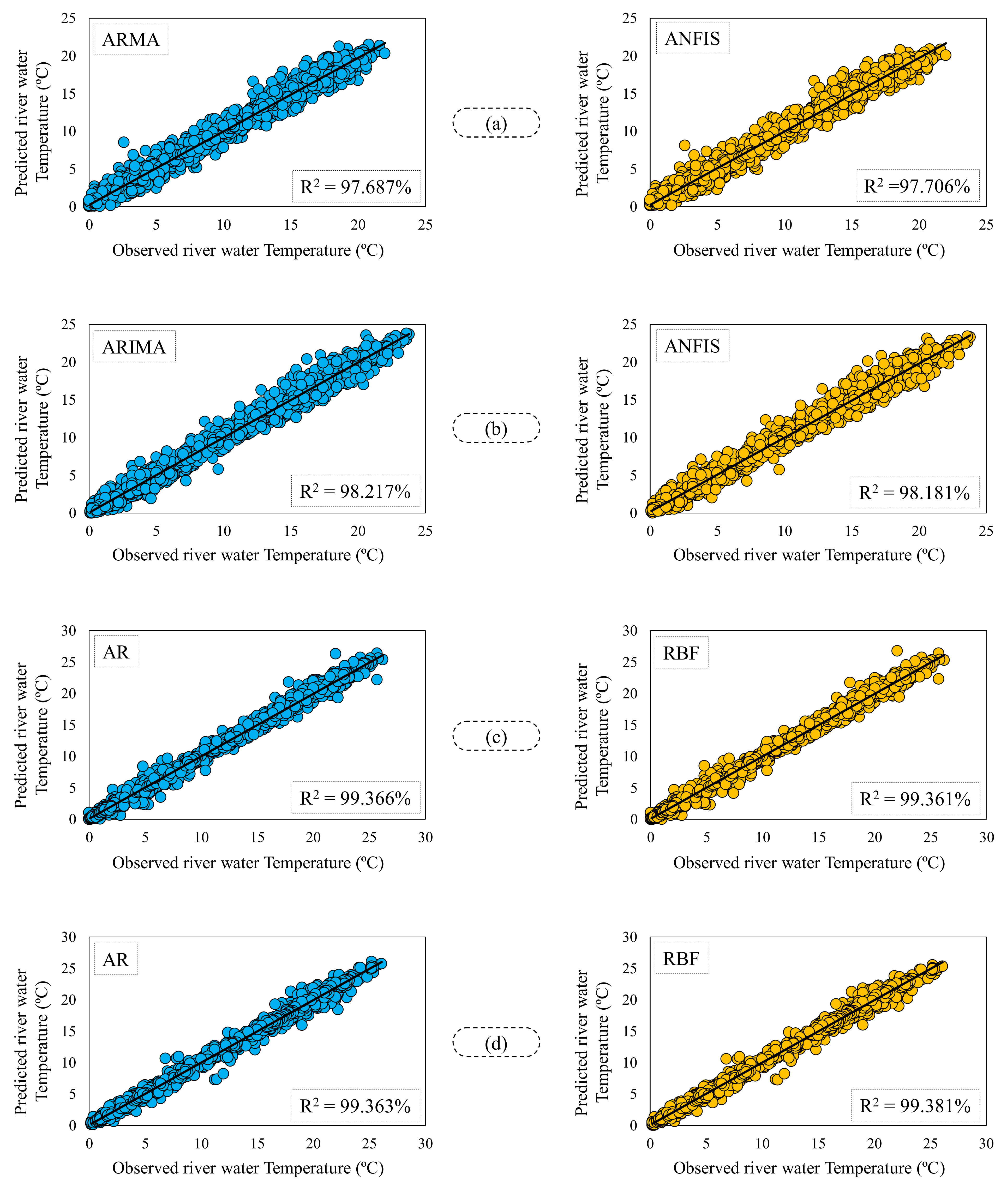
The evaluation in this step is performed using the RMSE and MAE criteria (Table 2). Since the validity of the numerical models is specified during their test periods, in this table we discuss the test phase for the stations. At first glance, we can see partial differences between the AI and the stochastics. Among the stochastic methods, the MA had the highest prediction errors, but the others—including AR, ARMA and ARIMA—had better performance. Among the AI methods, the best performance was displayed by the ANFIS and RBF models, with the GMDH was the weakest AI model. For the Bobry station, ARMA was the best stochastic model, with RMSE = 0.920 °C and MAE = 0.690 °C, while ANFIS with inputs of ACF had the highest accuracy among AIs (RMSE = 0.916 °C and MAE = 0.694 °C). In a similar scenario for the Sieradz station, the ANFIS was reported as the best AI, and the ARIMA as the best stochastic model. For the Poznań and Gorzow Wielkopolski stations, the criteria values were less than for the previous stations (RMSE values of about 0.6 °C and MAE of about 0.4 °C), and the AR and RBF models were the best among the stochastic and AI models, respectively. Furthermore, there was no significant reported superiority when comparing ACF and PACF input selectors. Scatter plots were drawn to make a graphical comparison between the prediction results of the stochastics and the AIs (Figure 7).
Figure 7 shows the scatter plots for predicted TRW and its actual observations. In Figure 7, the best-performing stochastic models are shown on the left, and the best AIs on the right. These graphs demonstrate that predictions are correlate significantly with observed TRW at all stations. The R2 values are above 97%, and the dots come together well around the fitted regression line. In all cases, the R2 values of the stochastics and AIs are too close, and the differences are partial (in the 1st or even 2nd decimal place of R2). In this comparison, therefore, the linear stochastic models can be considered more suitable due to their simplicity. The best R2 value is 99.381%, and was obtained for the RBF model at the Gorzow Wielkopolski stations. The weakest R2 value—97.687%—was determined for the ARMA model at the Bobry station.

3.2. Investigating the Models in Extreme TRW Deciles

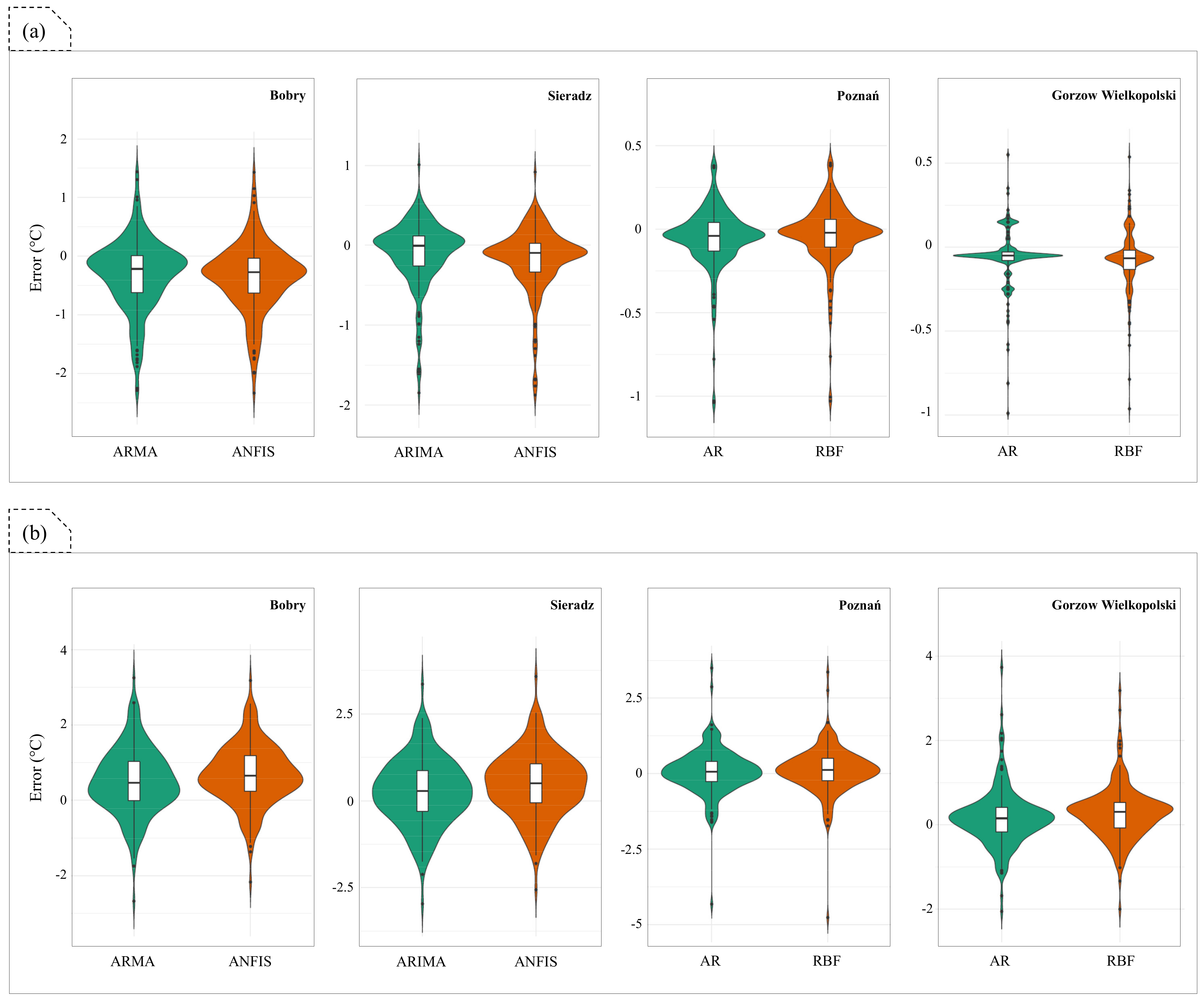
To investigate the prediction abilities of the used models in extreme events, the highest and lowest TRW deciles were separated in the test period. Next, their error distributions were determined, and are shown as violin plots (Figure 8).
Figure 8 presents a selection of the best stochastic and AI models (according to the bold rows of Table 2), with violin plots drawn separately for the highest and lowest deciles, by station. On the basis of the vicinity of the violins’ main curvature to the Error = 0 °C line, it is demonstrated that all the models are suitable for both of the extreme deciles. A comparison of the models makes it obvious that the violins’ main curvatures in stochastic models are somewhat closer to the Error = 0 line than in AI models. The clearest examples of this are the Bobry and Sieradz stations in the lowest decile, and the Bobry and Gorzow Wielkopolski stations in the highest decile. When comparing the two studied deciles, we see clearly that the violins are wider in the highest decile and more acute in the lowest. This demonstrates that the lowest TRW decile has less errors and can achieve better predictions through numerical models than the highest decile. If looked at from another perspective, the plots (Figure 8) generally show that the curvatures are sharper for Poznań and Gorzow Wielkopolski stations, which indicates that the TRW at these two stations offers better predictions than at Bobry and Sieradz.
A Spearman non-parametric correlation test was also implemented between the observations and the predictions. This test was applied seamlessly for all of the stations. The consequent correlation matrix is shown in Table 3.
This non-parametric statistical test (Table 3) says that the predictions are significantly correlated at the 0.01 level. In the upper decile, the correlations are stronger than in the lower decile. In both deciles, the predictions of MA are reported to be the weakest correlated outputs (0.607 and 0.759) against the observations. Additionally, the greatest difference between the models is established as being between MA and GMDH, leading to correlation coefficients of 0.735 and 0.878 for the lower and upper deciles, respectively. However, in general, the correlations are high, and this indicates that there are no significant differences between the models’ predictions with respect to extreme events of water temperature.

3.3. Comparing Prediction Performance between Stations

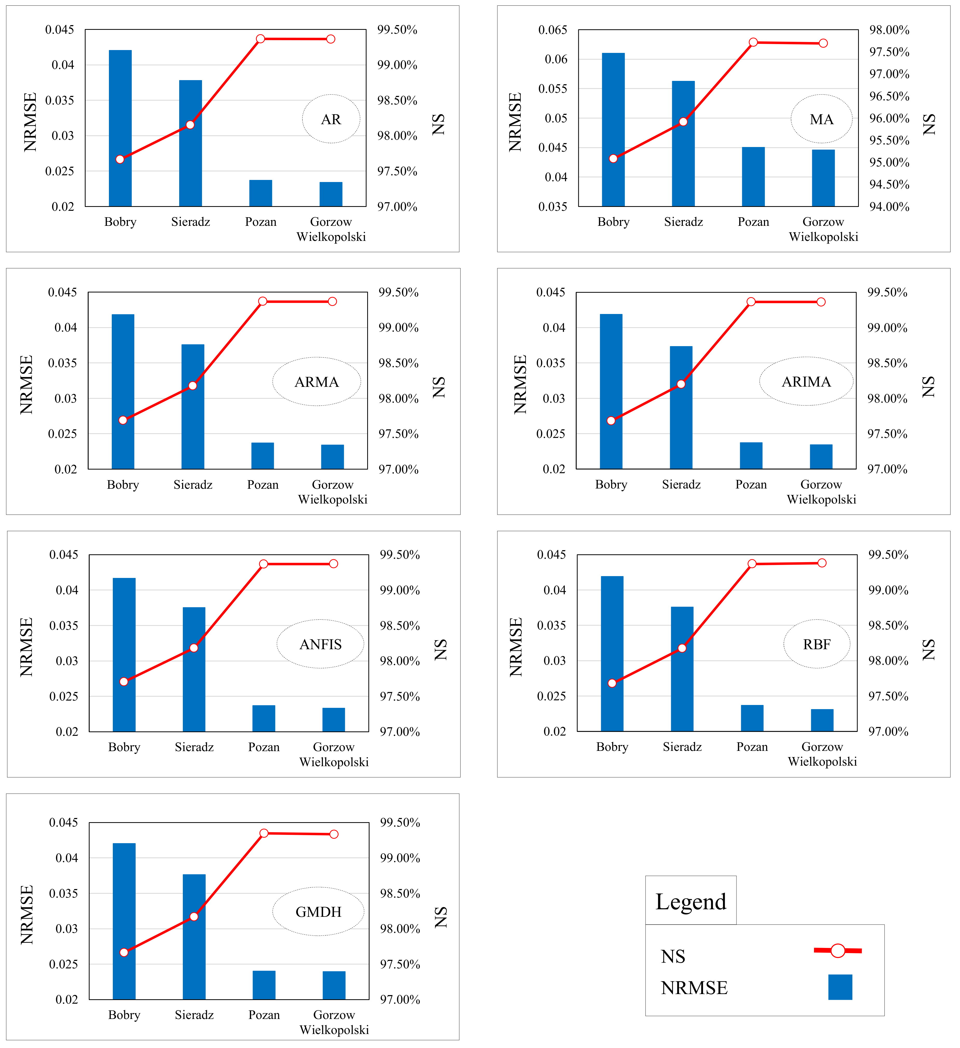
The ranges of TRW differ at the four stations (Table 1). The NRMSE is a normalized form of the RMSE, and considers the range of the observation dataset and is a good measurement for making a comparison between different ranged datasets. In this step, the prediction accuracies were investigated using NRMSE and NS criteria. For this purpose, the combined line-bar chart was used for the test period of all seven studied models (Figure 9).
At first glance, it is obvious that in all seven models, the NRMSE values have a decreasing trend, and NS values have an increasing trend at the stations. This indicates that the Bobry and Sieradz stations have lower prediction accuracies than the Poznań and Gorzow Wielkopolski stations. As a matter of fact, predictions offered by the models improve as we proceed downstream along the catchment area.
In the case of the Warta River, which constitutes the object of study, better prediction results for TRW were obtained for the middle and lower sections of its course (for the Poznań and Gorzow Wielkopolski water gauges), and slightly worse results were obtained for the water gauges located along the upper course (Bobry and Sieradz). Differences in the effectiveness of the prediction models may result from the influence of local factors modifying the features of both the thermal regime and the runoff regime, influencing, for example, an increase in the variability and irregularity of flow. Figure 10 shows the time series plots of best predicted values and their observations in both training and testing periods of the stations. As can be seen, in downstream stations (Bobry and Sieradz), there are more significant overlaps than in upstream ones (Poznań and Gorzow Wielkopolski).
Research on the trend of changes in TRW in Poland, carried out by Graf and Wrzesiński [80], identified water gauges on the Warta River in which the observation series of TRW showed an opposite trend of changes compared to the rest of the country. In most cases, these are located along sections of the river that are subjected to anthropopressure, such as a retention reservoir, municipal wastewater discharges, or modifications of the way in which the valley is used. The Bobry and Sieradz water gauges (upper section of the river course) are located on the river above the Jeziorsko Reservoir, which was built to regulate flows on the river. In its upper reaches, the river shows greater flow variability and greater irregularity, which may affect the modification of TRW distribution and, consequently, void the prediction results. The impact of anthropogenic influences on the structure of the Warta River TRW measurement series has been confirmed in research performed by, among others, [80,81,82,83].

4. Discussion

In the prediction made for daily TRW in the Warta River, different results were obtained when using the stochastic and AI models. As emphasized by Zhu and Piotrowski [3], comparisons of the results of models used to forecast the TRW have not been entirely conclusive. This problem is also indicated by the results of studies assessing the possibilities of predicting the characteristics of the thermal regime of rivers using various statistical models and artificial intelligence [3,22,34,84,85]. This is the result of various assumptions and limitations in the use of methods, input data for modeling, the level of data resolution, and the length of the observation series [54].
According to Qiu et al. [86], machine learning models perform well in TRW modeling, offering a very accurate empirical basis for its prediction. Zhu et al. [21,34] used different versions of methods to predict daily TRW: the Forward Neural Network (FFNN), Gaussian Process Regression (GPR) and the Decision Tree (DT), demonstrating that these models had similar performance when only air temperature was used as a predictor. Additionally, when the day of the year was included as an input, the performance of the three machine learning models improved significantly. As Graf [54] emphasized, TRW as a forecast variable also depends on its values in previous periods, which is related to the long memory of the system.
In the predictive TRW models developed for the Warta River, we included daily temperature delays as an input variable. According to Santos-Fernandez et al. [87], when the purpose of the application of the stochastic method is time interpolation and forecasting of future TRW values at the locations of measuring points (water gauges), and there is no need to describe unique spatial relationships on streams, thermal conditions reflect the standard models of time series.
The most favorable TRW forecasts in the upper section of the Warta River were obtained through the ARMA (Beaver station) and ARIMA (Sieradz) stochastic models, and the ANFIS AI model. However, for the middle (Poznań) and lower (Gorzow Wielkopolski) sections of the river, the best predictions were given by the AR model (among the stochastic models) and the RBFNN model among the AI models. The weakest predictive effects were obtained through the GMDH model, which can be associated with its optimization. The validity of using the first-order autoregressive model AR (1) for predicting TRW has been demonstrated, among others, by [10,88,89], while the Autoregressive Integrated Moving Average (ARIMA) was applied by Graf [54]. According to Santos-Fernandez et al. [87], in practice, in order to fit a model that is simple and generates precise estimates of fixed effects in predicting TRW, the AR model should be applied.
In the literature, there is a study authored by Graf et al. [22], which predicted the TRW of the Warta River. The researchers investigated the present four hydrometric stations, but used different machine learning approaches. Their best fitted model was the Wavelet Multilayer Perceptron Neural Network (WTMLPNN). When comparing similar hydrometric stations, the RMSE and MAE values show that the models implemented in the current study have superior performance. For example, at Bobry station, Graf et al. [22] obtained RMSE = 1.217 °C and MAE = 0.930 °C using WTMLPNN, which is less commonly reported through ANFIS in the current study (RMSE = 0.916 °C and MAE = 0.694 °C). Additionally, Graf et al. [22] and the present study obtained a similar comparison result for the Sieradz station; RMSE = 0.981 °C and MAE = 0.781 °C through WTMLPNN in [22] and RMSE = 0.889 °C and MAE = 0.652 °C through ANFIS in the current study. Furthermore, at the Poznań and Gorzow Wielkopolski stations, the current RBF model worked better than the WTMLPNN employed by Graf et al. [22]. In general, the AIs (including the ANFIS and the RBF) used in the present study achieve a superiority of 58.7% over the WTMLPNN. The reason for this seems to be related to the nature of temperature data. The temperature time series display a strong linear autocorrelation, and this linear relation can be better realized by simpler models. As we see in this comparison, the WTMLPNN is an MLP model with a large number of parameters (including the number of hidden layers, the number of neurons in individual layers, and the type of the transfer function in each neuron) combined by wavelet analysis, while the ANFIS has just one (number of clusters), and the RBF only two parameters (spread and the maximum number of neurons). Another difference between [22] and the current study is that the latter used stochastic methods, and in some instances (the Sieradz station, for example), these performed better than the AIs. The superiority of stochastic models in relation to AIs for temperature forecasting has also been reported for the short- and long-term forecasting of air temperature. Aghelpour et al. [39] also demonstrated that in different climates air temperature was better forecast by linear stochastic models than the complex AI and meta-innovative models; again, this shows the nature of linear autocorrelation in temperature time series.
Cole et al. [90] found the MLPNN to be better than a heat budget approach. Hong and Bhamidimarri [91] determined that the DNFIS model was superior not only to the classical ANFIS, but also to the MLPNN, at least in terms of short-term TRW forecasting. Zhu et al. [32] compared the performance of the MLPNN and ANFIS models, indicating that the MLPNN model provides the best overall performance, and that the choice of identification method significantly affects the performance of the ANFIS model. The applicability of the ANFIS model for forecasting TRW is quite restricted, although ANFIS are of great use in other research applications [90,92,93]. In another study, Zhu et al. [21] showed that the coupled neural network performs better than the GPR and DT models. According to Piotrowski et al. [31], the choice of a neural network depends on the method of comparing models.

5. Conclusions

The investigations show promising results in predicting daily TRW. The results can be summarized in the following points:
  • Both AI and stochastic model types had acceptable performance in predicting daily TRW.
  • Among the stochastic methods, the AR, ARMA and ARIMA, and among the AI methods, the ANFIS and RBF, offered the best-fitted predictions of TRW. The performance difference between these two types of models is very small, and indeed negligible.
  • The stochastic models have less prediction errors in extreme TRW events.
The general results of comparisons show the superiority of the linear stochastic models, due to simplicity and parsimony. Additionally, AI models with fewer parameters (ANFIS and RBF) offered better results than those that were more complex and had large numbers of parameters (GMDH). In fact, it can be stated that for the purposes of forecasting TRW, the simpler the model, the more appropriate and logical is its use; as can be seen for the Poznań and Gorzow Wielkopolski stations, the AR(2) model—a simple linear regression model with just two input variables—was the best variant. The study confirms the applicability of these numerical approaches for the current river basin, and that they have research value for other catchment areas (among others, in order to extend the results). Furthermore, it is suggested that future researchers use optimization algorithms, such as Genetic, Particle swarm, dragonfly, etc., hybridized by the Ais, to improve the abilities of the AI models. To examine the impacts of global warming and climate change on TRW, it is a possibility to use the meteorological variables for long-term future periods, which could be another suggestion for the long-term forecasting of the variable TRW.

Author Contributions

Conceptualization, R.G. and P.A.; methodology, R.G. and P.A.; software, P.A.; validation, P.A.; formal analysis, P.A.; investigation, R.G.; resources, R.G.; data curation, R.G.; writing—original draft preparation, R.G. and P.A.; writing—review and editing, R.G.; visualization, P.A.; supervision, R.G. All authors have read and agreed to the published version of the manuscript.

Funding

This research received no external funding.

Institutional Review Board Statement

Not applicable.

Informed Consent Statement

Not applicable.

Data Availability Statement

The data that support the findings of this study are available from the corresponding author upon reasonable request.

Acknowledgments

The authors thank their universities for their support. Acknowledgments to the Institute of Meteorology and Water Management–National Research Institute (IMWM-NRI, Warsaw, Poland) for the release of the output database.

Conflicts of Interest

The authors declare no conflict of interest.

References

  1. Arismendi, I.; Safeeq, M.; Dunham, J.B.; Johnson, S.L. Can air temperature be used to project influences of climate change on stream temperature? Environ. Res. Lett. 2014, 9, 084015. [Google Scholar] [CrossRef]
  2. Allan, J.D.; Castillo, M.M. Stream Ecology: Structure and Function of Running Waters, 2nd ed.; Chapman and Hall: New York, NY, USA, 2007. [Google Scholar]
  3. Zhu, S.; Piotrowski, A.P. River/stream water temperature forecasting using artificial intelligence models: A systematic review. Acta Geophys. 2020, 68, 1433–1442. [Google Scholar] [CrossRef]
  4. Langan, S.J.; Johnston, L.; Donaghy, M.J.; Youngson, A.F.; Hay, D.W.; Soulsby, C. Variation in river water temperatures in an upland stream over a 30-year period. Sci. Total. Environ. 2001, 265, 195–207. [Google Scholar] [CrossRef]
  5. Liu, B.; Yang, D.; Ye, B.; Berezovskaya, S. Long-term open-water season stream temperature variations and changes over Lena River Basin in Siberia. Glob. Planet. Chang. 2005, 48, 96–111. [Google Scholar] [CrossRef] [Green Version]
  6. Arora, R.; Tockner, K.; Venohor, M. Changing river temperatures in northern Germany: Trends and drivers of change. Hydrol. Process. 2016, 30, 3084–3096. [Google Scholar] [CrossRef]
  7. Basarin, B.; Luki’c, T.; Pavi’c, D.; Wilby, R.L. Trends and multi-annual variability of water temperatures in the river Danube, Serbia. Hydrol. Process. 2016, 30, 3315–3329. [Google Scholar] [CrossRef] [Green Version]
  8. Brosofske, K.D.; Chen, J.; Naiman, R.J.; Franklin, J.F. Harvesting effects on microclimatic gradients from small streams to uplands in western Washington. Ecol. Appl. 1997, 7, 1188–1200. [Google Scholar] [CrossRef]
  9. Sahoo, G.B.; Schladow, S.G.; Reuter, J.E. Forecasting stream water temperature using regression analysis, artificial neural network, and chaotic non-linear dynamic models. J. Hydrol. 2009, 378, 325–342. [Google Scholar] [CrossRef]
  10. Letcher, B.H.; Hocking, D.J.; O’Neil, K.; Whiteley, A.R.; Nislow, K.H.; O’Donnell, M.J. A hierarchical model of daily stream temperature using air-water temperature synchronization, autocorrelation, and time lags. PeerJ 2016, 4, e1727. [Google Scholar] [CrossRef] [Green Version]
  11. Graf, R.A. Multifaceted analysis of the relationship between daily temperature of river water and air. Acta Geophys. 2019, 67, 905–920. [Google Scholar] [CrossRef] [Green Version]
  12. Graf, R.; Wrzesiński, D. Relationship between Water Temperature of Polish Rivers and Large-Scale Atmospheric Circulation. Water 2019, 11, 1690. [Google Scholar] [CrossRef] [Green Version]
  13. Pilgrim, J.M.; Fang, X.; Stefan, H.G. Stream temperature correlations with air temperatures in Minnesota: Implications for climate warming. J. Am. Water Resour. Assoc. 1998, 34, 1109–1121. [Google Scholar] [CrossRef]
  14. Caissie, D.; El-Jabi, N.; Satish, M.G. Modelling of maximum daily water temperatures in a small stream using air temperatures. J. Hydrol. 2001, 251, 14–28. [Google Scholar] [CrossRef]
  15. Caissie, D.; St-Hilaire, A.; El-Jabi, N. Prediction of Water Temperatures Using Regression and Stochastic Models. In Proceedings of the 57th Canadian Water Resources Association Annual Congress, Montreal, QC, Canada, 16–18 June 2004. [Google Scholar]
  16. Webb, B.W.; Clack, P.D.; Walling, D.E. Water-air temperature relationships in a Devon river system and the role of flow. Hydrol. Process. 2003, 17, 3069–3084. [Google Scholar] [CrossRef]
  17. Morrill, J.C.; Bales, R.C.; Conklin, M.H. Estimating stream temperature from air temperature: Implications for future water quality. J. Environ. Eng. 2005, 131, 139–146. [Google Scholar] [CrossRef] [Green Version]
  18. Hilderbrand, R.H.; Kashiwagi, M.T.; Prochaska, A.P. Regional and local scale modeling of stream temperatures and spatio-temporal variation in thermal sensitivities. Environ. Manag. 2014, 54, 14–22. [Google Scholar] [CrossRef] [PubMed]
  19. Li, H.; Deng, X.; Kim, D.-Y.; Smith, E.P. Modeling maximum daily temperature using a varying coefficient regression model. Water Resour. Res. 2014, 50, 3073–3087. [Google Scholar] [CrossRef]
  20. Zhu, S.; Heddam, S.; Wu, S.; Dai, J.; Jia, B. Extreme learning machine-based prediction of daily water temperature for rivers. Environ. Earth Sci. 2019, 78, 202. [Google Scholar] [CrossRef]
  21. Zhu, S.; Nyarko, E.K.; Hadzima-Nyarko, M.; Heddam, S.; Wu, S. Assessing the performance of a suite of machine learning models for daily river water temperature prediction. PeerJ 2019, 7, e7065. [Google Scholar] [CrossRef] [PubMed]
  22. Graf, R.; Zhu, S.; Sivakumar, B. Forecasting river water temperature time series using a wavelet–neural network hybrid modelling approach. J. Hydrol. 2019, 578, 124115. [Google Scholar] [CrossRef]
  23. Napiórkowski, M.J.; Piotrowski, A.P.; Napiórkowski, J.J. Stream Temperature Forecasting by Means of Ensemble of Neural Networks: Importance of Input Variables and Ensemble Size; Schleiss, A.J., De Cesare, G., Franca, M.J., Pfister, M., Eds.; River Flow, Taylor & Francis Group: London, UK, 2014. [Google Scholar]
  24. Piccolroaz, S.; Calamita, E.; Majone, B.; Gallice, A.; Siviglia, A.; Toffolon, M. Prediction of river water temperature: A comparison between a new family of hybrid models and statistical approaches. Hydrol. Process. 2016, 30, 3901–3917. [Google Scholar] [CrossRef]
  25. Zhu, S.; Heddam, S. Prediction of dissolved oxygen in urban rivers at the Three Gorges Reservoir, China: Extreme learning machines (ELM) versus artificial neural network (ANN). Water Qual. Res. J. 2020, 55, 106–118. [Google Scholar] [CrossRef]
  26. Zhu, S.; Heddam, S.; Nyarko, E.K.; Hadzima-Nyarko, M.; Piccolroaz, S.; Wu, S. Modeling daily water temperature for rivers: Comparison between adaptive neuro-fuzzy inference systems and artificial neural networks models. Environ. Sci. Pollut. Res. 2019, 26, 402–420. [Google Scholar] [CrossRef]
  27. Piotrowski, A.P.; Napiórkowski, M.J.; Piotrowska, A.E. Impact of deep learning-based dropout on shallow neural networks applied to stream temperature modelling. Earth-Sci. Rev. 2020, 201, 103076. [Google Scholar] [CrossRef]
  28. Daigle, A.; St-Hilaire, A.; Ouellet, V.; Corriveau, J.; Taha, B.M.J.; Ouarda, L.B. Diagnostic study and modeling of the annual positive water temperature onset. J. Hydrol. 2009, 370, 29–38. [Google Scholar] [CrossRef]
  29. Faruk, D.O. A hybrid neural network and ARIMA model for water quality time series prediction. Eng. Appl. Artif. Intell. 2010, 23, 586–594. [Google Scholar] [CrossRef]
  30. Tao, W.; Kailin, Y.; Yongxin, G. Application of artificial neural networks to forecasting ice conditions of the Yellow River in the Inner Mongolia reach. J. Hydrol. Eng. ASCE 2008, 13, 811–816. [Google Scholar] [CrossRef]
  31. Piotrowski, A.P.; Napiórkowski, M.J.; Napiórkowski, J.J.; Osuch, M. Comparing various artificial neural network types for water temperature prediction in rivers. J. Hydrol. 2015, 529, 302–315. [Google Scholar] [CrossRef]
  32. Zhu, S.; Hadzima-Nyarko, M.; Gao, A.; Wang, F.; Wu, J.; Wu, S. Two hybrid data-driven models for modeling water-air temperature relationship in rivers. Environ. Sci. Pollut. Res. 2019, 26, 12622–12630. [Google Scholar] [CrossRef] [PubMed]
  33. Caissie, D.; El-Jabi, N.; St-Hilaire, A. Stochastic modelling of water temperature in a small stream using air to water relations. Can. J. Civ. Eng. 1998, 25, 250–260. [Google Scholar] [CrossRef]
  34. Zhu, S.; Nyarko, E.K.; Hadzima-Nyarko, M. Modelling daily water temperature from air temperature for the Missouri River. PeerJ 2018, 6, e4894. [Google Scholar] [CrossRef] [Green Version]
  35. Ahmadi-Nedushan, B.; St-Hilaire, A.; Ouarda, T.B.M.J.; Bilodeau, L.; Robichaud, É.; Thiémonge, N.; Bobée, B. Predicting river water temperatures using stochastic models: Case study of the Moisie river (Quebec, Canada). Hydrol. Process. 2007, 21, 21–34. [Google Scholar] [CrossRef]
  36. Hadzima-Nyarko, M.; Rabi, A.; Śperac, M. Implementation of artificial neural networks in modeling the water-air temperature relationship of the river Drava. Water Resour. Manag. 2014, 28, 1379–1394. [Google Scholar] [CrossRef]
  37. Rabi, A.; Hadzima-Nyarko, M.; Sperac, M. Modelling river temperature from air temperature in the River Drava (Croatia). Hydrol. Sci. J. 2015, 60, 1490–1507. [Google Scholar] [CrossRef]
  38. Benyahya, L.; St-Hilaire, A.; Ouarda, T.B.M.J.; Bobée, B.; Dumas, J. Comparison of nonparametric and parametric water temperature models on the Nivelle River, France. Hydrol. Sci. J. 2008, 53, 640–655. [Google Scholar] [CrossRef] [Green Version]
  39. Aghelpour, P.; Mohammadi, B.; Biazar, S.M. Long-term monthly average temperature forecasting in some climate types of Iran, using the models SARIMA, SVR, and SVR-FA. Theor. Appl. Climatol. 2019, 138, 1471–1480. [Google Scholar] [CrossRef]
  40. Ashrafzadeh, A.; Kişi, O.; Aghelpour, P.; Biazar, S.M.; Masouleh, M.A. Comparative study of time series models, support vector machines, and GMDH in forecasting long-term evapotranspiration rates in northern Iran. J. Irrig. Drain. Eng. 2020, 146, 04020010. [Google Scholar] [CrossRef]
  41. Aghelpour, P.; Bahrami-Pichaghchi, H.; Varshavian, V. Hydrological drought forecasting using multi-scalar streamflow drought index, stochastic models and machine learning approaches, in northern Iran. Stoch. Environ. Res. Risk Assess. 2021, 35, 1615–1635. [Google Scholar] [CrossRef]
  42. Aghelpour, P.; Singh, V.P.; Varshavian, V. Time series prediction of seasonal precipitation in Iran, using data-driven models: A comparison under different climatic conditions. Arab. J. Geosci. 2021, 14, 551. [Google Scholar] [CrossRef]
  43. Box, G.E.P.; Jenkins, G. Time Series Analysis: Forecasting and Control, 2nd ed.; Holden-Day Publishments: San Fransisco, CA, USA, 1976. [Google Scholar]
  44. Du, H.; Zhao, Z.; Xue, H. ARIMA-M: A New Model for Daily Water Consumption Prediction Based on the Autoregressive Integrated Moving Average Model and the Markov Chain Error Correction. Water 2020, 12, 760. [Google Scholar] [CrossRef] [Green Version]
  45. Jothiprakash, V.; Kote, A.S. Improving the performance of data-driven techniques through data pre-processing for modelling daily reservoir inflow. Hydrol. Sci. J. 2011, 56, 168–186. [Google Scholar] [CrossRef]
  46. Modarres, R.; Ouarda, T.B. Modelling heteroscedasticty of streamflow times series. Hydrol. Sci. J. 2013, 58, 54–64. [Google Scholar] [CrossRef]
  47. Lippi, M.; Bertini, M.; Frasconi, P. Short-term traffic flow forecasting: An experimental comparison of time-series analysis and supervised learning. IEEE Trans. Intell. Transp. Syst. 2013, 14, 871–882. [Google Scholar] [CrossRef]
  48. Abudu, S.; Cui, C.; King, J.P.; Abudukadeer, K. Comparison of performance of statistical models in forecasting monthly streamflow of Kizil River, China. Water Sci. Eng. 2010, 3, 269–281. [Google Scholar]
  49. Valipour, M.; Banihabib, M.E.; Behbahani, S.M.R. Comparison of the ARMA, ARIMA, and the autoregressive artificial neural network models in forecasting the monthly inflow of Dez dam reservoir. J. Hydrol. 2013, 476, 433–441. [Google Scholar] [CrossRef]
  50. Aghelpour, P.; Varshavian, V. Evaluation of stochastic and artificial intelligence models in modeling and predicting of river daily flow time series. Stoch. Environ. Res. Risk Assess. 2020, 34, 33–50. [Google Scholar] [CrossRef]
  51. Khosravi, K.; Golkarian, A.; Booij, M.J.; Barzegar, R.; Sun, W.; Yaseen, Z.M.; Mosavi, A. Improving daily stochastic streamflow prediction: Comparison of novel hybrid data mining algorithms. Hydrol. Sci. J. 2021, 66, 1457–1474. [Google Scholar] [CrossRef]
  52. Bari, M.F.; Islam, K.M.S. Stochastic model of flow duration curves for selected rivers in Bangladesh. In Climate Variability and Change–Hydrological Impacts, Proceedings of the Fifth FRIEND World Conference, Havana, Cuba, 27 November–1 December 2006; IAHS Publ.: Wallingford, UK, 2006; Volume 308, pp. 99–104. [Google Scholar]
  53. Papalaskaris, T.; Kampas, G. Time series analysis of water characteristics of streams in Eastern Macedonia—Thrace, Greece. Eur. Water 2017, 57, 93–100. [Google Scholar]
  54. Graf, R. Distribution properties of a measurement series of river water temperature at different time resolution levels (based on the example of the Lowland River Notec, Poland). Water 2018, 10, 203. [Google Scholar] [CrossRef] [Green Version]
  55. Shvartser, L.; Shamir, U.; Feldman, M. Forecasting hourly water demands by pattern recognition approach. J. Water Resour. Plan. Manag. 1993, 119, 611–627. [Google Scholar] [CrossRef]
  56. Mombeni, H.A.; Rezaei, S.; Nadarajah, S.; Emami, M. Estimation of water demand in Iran based on sarima models. Environ. Model. Assess. 2013, 18, 559–565. [Google Scholar] [CrossRef]
  57. Woś, A. The Climate of Poland in the Second Half of the 20th Century; Scientific Publishing House UAM: Poznan, Poland, 2010; p. 490. (In Polish) [Google Scholar]
  58. Salas, J.D.; Delleur, J.W.; Yevjevich, V.; Lane, W.L. Applied Modelling of Hydrologic Time Series; Water Resource Publications: Littleton, CO, USA, 1980; p. 484. [Google Scholar]
  59. Mohammadi, B.; Linh, N.T.; Pham, Q.B.; Ahmed, A.N.; Vojteková, J.; Guan, Y.; Abba, S.I.; El-Shafie, A. Adaptive neuro-fuzzy inference system coupled with shuffled frog leaping algorithm for predicting river streamflow time series. Hydrol. Sci. J. 2020, 65, 1738–1751. [Google Scholar] [CrossRef]
  60. Jang, J.S.R.; Sun, C.T.; Mizutani, E. Neuro-fuzzy and soft computing: A computational approach to learning and machine intelligence. IEEE Trans. Autom. Control 1997, 42, 1482–1484. [Google Scholar] [CrossRef]
  61. Nourani, V.; Alami, M.T.; Vousoughi, F.D. Self-organizing map clustering technique for ANN-based spatiotemporal modeling of groundwater quality parameters. J. Hydroinform. 2016, 18, 288–309. [Google Scholar] [CrossRef]
  62. Fallah-Mehdipour, E.; Haddad, O.B.; Marino, M.A. Genetic programming in groundwater modeling. J. Hydrol. Eng. 2014, 19, 04014031. [Google Scholar] [CrossRef]
  63. Kisi, O.; Demir, V.; Kim, S. Estimation of long-term monthly temperatures by three different adaptive neuro-fuzzy approaches using geographical inputs. J. Irrig. Drain. Eng. 2017, 143, 04017052. [Google Scholar] [CrossRef]
  64. Çaydaş, U.; Hasçalık, A.; Ekici, S. An adaptive neuro-fuzzy inference system (ANFIS) model for wire-EDM. Expert Syst. Appl. 2009, 36, 6135–6139. [Google Scholar] [CrossRef]
  65. Mamdani, E.H.; Assilian, S. An experiment in linguistic synthesis with a fuzzy logic controller. Int. J. Manmach. Stud. 1975, 7, 1–13. [Google Scholar] [CrossRef]
  66. Takagi, T.; Sugeno, M. Fuzzy identification of systems and its applications to modeling and control. IEEE Trans. Syst. Man Cybern. 1985, 15, 116–132. [Google Scholar] [CrossRef]
  67. Aghelpour, P.; Mohammadi, B.; Mehdizadeh, S.; Bahrami-Pichaghchi, H.; Duan, Z. A novel hybrid dragonfly optimization algorithm for agricultural drought prediction. Stoch. Environ. Res. Risk Assess. 2021, 1–19. [Google Scholar] [CrossRef]
  68. Parsaie, A. Predictive modeling the side weir discharge coefficient using neural network. Model. Earth Syst. Environ. 2016, 2, 63. [Google Scholar] [CrossRef] [Green Version]
  69. Ehteshami, M.; Farahani, N.D.; Tavassoli, S. Simulation of nitrate contamination in groundwater using artificial neural networks. Model. Earth Syst. Environ. 2016, 2, 28. [Google Scholar] [CrossRef] [Green Version]
  70. Heddam, S. New modelling strategy based on radial basis function neural network (RBFNN) for predicting dissolved oxygen concentration using the components of the Gregorian calendar as inputs: Case study of Clackamas River, Oregon, USA. Model. Earth Syst. Environ. 2016, 2, 167. [Google Scholar] [CrossRef] [Green Version]
  71. Alizamir, M.; Kisi, O.; Zounemat-Kermani, M. Modelling long-term groundwater fluctuations by extreme learning machine using hydro-climatic data. Hydrol. Sci. J. 2018, 63, 63–73. [Google Scholar] [CrossRef]
  72. Ivakhnenko, A.G. Heuristic self-organization in problems of engineering cybernetics. Automatica 1970, 6, 207–219. [Google Scholar] [CrossRef]
  73. Aghelpour, P.; Kisi, O.; Varshavian, V. Multivariate Drought Forecasting in Short-and Long-Term Horizons Using MSPI and Data-Driven Approaches. J. Hydrol. Eng. 2021, 26, 04021006. [Google Scholar] [CrossRef]
  74. Najafzadeh, M.; Barani, G.-A. Comparison of group method of data handling based genetic programming and back propagation systems to predict scour depth around bridge piers. Sci. Iran. A 2011, 18, 1207–1213. [Google Scholar] [CrossRef]
  75. Pereira, I.M.; Bueno, E.I. Variable Identification in Group Method of Data Handling Methodology. In Proceedings of the International Nuclear Atlantic Conference—INAC 2011, Belo Horizonte, MG, Brazil, 24–28 October 2011; Associação Brasileira De Energia Nuclear—Aben: Rio de Janeiro, Brazil, 2011. [Google Scholar]
  76. Wang, M.; Rezaie-balf, M.; Naganna, S.R.; Yaseen, Z.M. Sourcing CHIRPS precipitation data for streamflow forecasting using Intrinsic Time-scale Decomposition based Machine Learning models. Hydrol. Sci. J. 2021, 66, 1437–1456. [Google Scholar] [CrossRef]
  77. Nelles, O. Nonlinear System Identification: From Classical Approaches to Neural Networks and Fuzzy Models; Springer: Berlin/Heidelberg, Germany, 2001. [Google Scholar]
  78. Zahraie, B.; Nasseri, M.; Nematizadeh, F. Exploring spatiotemporal meteorological correlations for basin scale meteorological drought forecasting using data mining methods. Arab. J. Geosci. 2017, 10, 419. [Google Scholar] [CrossRef]
  79. Moriasi, D.; Arnold, J.; Van Liew, M.; Bingner, R.; Harmel, R.; Veith, T. Model evaluation guidelines for systematic quantification of accuracy in watershed simulations. Trans. ASABE 2007, 50, 885–900. [Google Scholar] [CrossRef]
  80. Graf, R.; Wrzesiński, D. Detecting Patterns of Changes in River Water Temperature in Poland. Water 2020, 12, 1327. [Google Scholar] [CrossRef]
  81. Gorączko, M.; Pawłowski, B. Changing of ice phenomena on Warta river in vicinity of Uniejów. Biul. Uniejowski 2014, 3, 23–33. (In Polish) [Google Scholar]
  82. Graf, R. Variations of the Thermal Conditions of the Warta in the Profile Connecting the Urstromtal and Gorge Sections of the Valley (Nowa Wieś Podgórna—Śrem—Poznań). In Nowoczesne Metody i Rozwiązania w Hydrologii i Gospodarce Wodnej; Absalon, D., Matysik, M., Ruman, M., Eds.; Komisja Hydrologiczna PTG, Oddział: Katowice, Polska, 2015; pp. 177–194. (In Polish) [Google Scholar]
  83. Graf, R.; Łukaszewicz, J.T.; Jawgiel, K. The analysis of the structure and duration of ice phenomena on the Warta river in relation to thermic conditions in the years 1991–2010. Woda-Środowisko-Obsz. Wiej. 2018, 18, 5–28. (In Polish) [Google Scholar]
  84. Benyahya, L.; Caissie, D.; St-Hilaire, A.; Ouarda, T.B.M.; Bobée, B. A review of statistical water temperature models. Can. Water Resour. J. 2007, 32, 179–192. [Google Scholar] [CrossRef] [Green Version]
  85. Dugdale, S.J.; Hannah, D.M.; Malcolm, I.A. River temperature modelling: A review of process-based approaches and future directions. Earth-Sci. Rev. 2017, 175, 97–113. [Google Scholar] [CrossRef]
  86. Qiu, R.; Wang, Y.; Wang, D.; Qiu, W.; Wu, J.; Tao, Y. Water temperature forecasting based on modified artificial neural network methods: Two cases of the Yangtze River. Sci. Total Environ. 2020, 737, 139729. [Google Scholar] [CrossRef]
  87. Santos-Fernandez, E.; Ver Hoefc, J.M.; Petersona, E.E.; McGreea, J.; Isaak, D.J.; Mengersena, K. Bayesian spatio-temporal models for stream networks. arXiv 2021, arXiv:2103.03538v1. [Google Scholar]
  88. Bal, G.; Rivot, E.; Bagliniere, J.-L.; White, J.; Pr´evost, E. A hierarchical Bayesian model to quantify uncertainty of stream water temperature forecasts. PLoS ONE 2014, 9, e115659. [Google Scholar]
  89. Hague, M.J.; Patterson, D.A. Evaluation of statistical river temperature forecast models for fisheries management. N. Am. J. Fish. Manag. 2014, 34, 132–146. [Google Scholar] [CrossRef]
  90. Cole, J.C.; Maloney, K.O.; Schmid, M.; McKenna, J.E. Developing and testing temperature models for regulated systems: A case study on the upper Delaware River. J. Hydrol. 2014, 519, 588–598. [Google Scholar] [CrossRef]
  91. Hong, Y.S.T.; Bhamidimarri, R. Dynamic neuro-fuzzy local modeling system with a nonlinear feature extraction for the online adaptive warning system of river temperature affected by waste cooling water discharge. Stoch. Environ. Res. Risk Assess. 2012, 26, 947–960. [Google Scholar] [CrossRef]
  92. Kurnaz, S.; Cetin, O.; Kaynak, O. Adaptive neuro-fuzzy inference system based autonomous flight control of unmanned air vehicles. Expert Syst. Appl. 2010, 37, 1229–1234. [Google Scholar] [CrossRef]
  93. Mohandes, M.; Rehman, S.; Rahman, S.M. Estimation of wind speed profile using adaptive neuro-fuzzy inference system (ANFIS). Appl. Energy 2011, 8, 4024–4032. [Google Scholar] [CrossRef] [Green Version]
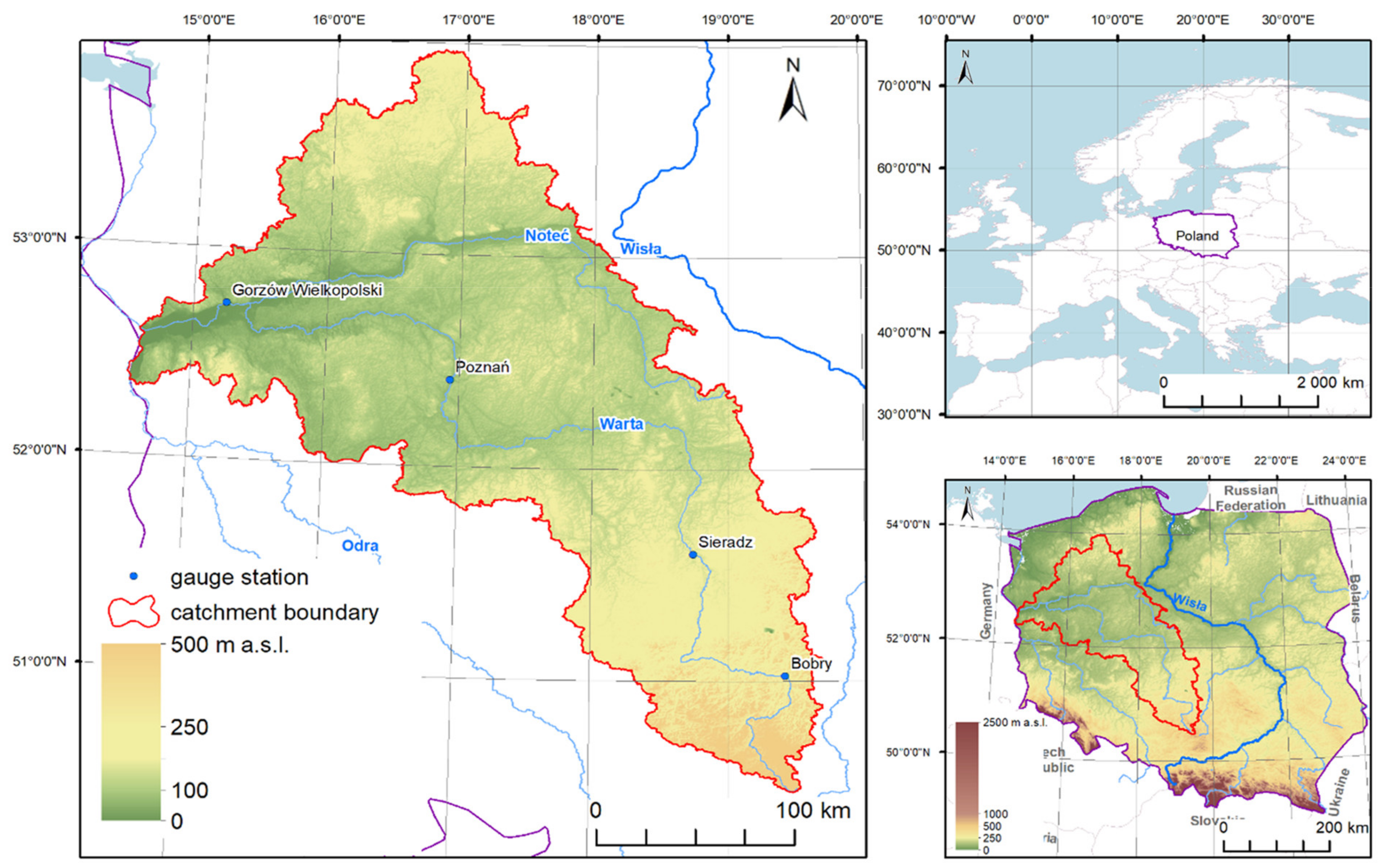
Figure 1. Map of the Warta River basin with the locations of hydrometric stations.
Atmosphere 12 01154 g001
Figure 2. Schematic structure of ANFIS model with two inputs.
Atmosphere 12 01154 g002
Figure 3. A simple structure of a multi-input RBF model.
Atmosphere 12 01154 g003
Figure 4. Schematic structure for a three-layered GMDH model.
Atmosphere 12 01154 g004
Figure 5. Flowchart of the modeling and prediction steps.
Atmosphere 12 01154 g005
Figure 6. Graphs of Autocorrelation (ACF) and Partial Autocorrelation (ACF) for the TRW time series. The alphabets refer to the hydrometric stations: (a) Bobry, (b) Sieradz, (c) Poznań and (d) Gorzow Wielkopolski.
Atmosphere 12 01154 g006
Figure 7. Scatter plots comparing the predictions of stochastic and artificial intelligence models, with their observation values (left side—the best model among stochastics; right side—the best model among artificial intelligences): (a) Bobry, (b) Sieradz, (c) Poznań and (d) Gorzow Wielkopolski.
Atmosphere 12 01154 g007
Figure 8. Violin plots to evaluate the error distributions in the lower (a) and upper deciles (b) of TRW.
Atmosphere 12 01154 g008
Figure 9. Comparing the TRW prediction accuracies between the hydrometric stations.
Atmosphere 12 01154 g009
Figure 10. Time series plots of the best predicted outputs of each station, beside its observed TRW.
Atmosphere 12 01154 g010
Table 1. The stations’ coordinate data and the specifications of the data under study.
Gauge
Station
CoordinatesPhase *Mean
(°C)
St. Dev. **
(°C)
C.V.
(%)
Min.
(°C)
Max.
(°C)
Skew.
(−)
Kurt.
(−)
Latitude
(°Northern)
Longitude
(°Eeastern)
Elevation
(m)
Bobry51.0219.40205.0Training9.76.162.30.0027.00.07−1.30
Testing9.96.061.10.0022.00.05−1.30
Sieradz51.6018.73130.5Training9.96.768.20.1024.80.10−1.33
Testing10.36.663.70.1023.80.09−1.26
Poznań52.3816.9354.5Training10.77.569.70.0026.20.11−1.44
Testing11.17.870.10.0026.20.08−1.41
Gorzow
Wielkopolski
52.7215.2325.0Training10.77.570.10.1026.10.10−1.41
Testing11.17.668.20.2026.10.06−1.41
* Phase: The first 15 years (1990-2004 hydrological years) belong to the training phase and the last 5 years (2005–2009 hydrological years) belong to the testing phase, ** Abbreviations: St. Dev. = standard deviation; C. V. = coefficient of variation; Min. = minimum; Max. = maximum; Skew. = skewness; Kurt. = kurtosis.
Table 2. Evaluating the implemented models for TRW prediction.
StationModelTrainingTesting
RMSE
(°C)
MAE
(°C)
RMSE
(°C)
MAE
(°C)
BobryAR (4)1.0270.7690.9240.692
MA (5)1.4621.1601.3421.084
ARMA (3,1) *1.0210.7650.9200.690
ARIMA (2,1,1)1.0220.7640.9210.691
ANFIS-ACF1.0140.7630.9160.694
ANFIS-PACF1.0240.7730.9240.697
RBF-ACF1.0100.7630.9220.698
RBF-PACF1.0240.7730.9240.697
GMDH-ACF1.0230.7680.9250.694
GMDH-PACF1.0330.7730.9310.694
SieradzAR (3)0.8690.6190.8960.669
MA (5)1.3231.0751.3331.071
ARMA (3,1)0.8640.6200.8900.666
ARIMA (4,1,4)0.8610.6140.8850.662
ANFIS-ACF0.8610.6140.8890.665
ANFIS-PACF0.8800.6320.9080.690
RBF-ACF0.8580.6140.8910.667
RBF-PACF0.8800.6320.9080.690
GMDH-ACF0.8650.6140.8920.664
GMDH-PACF0.8850.6330.9130.688
PoznańAR (3)0.4460.3060.6210.416
MA (5)0.9660.8091.1800.943
ARMA (2,1)0.4460.3060.6210.416
ARIMA (1,1,1)0.4470.3050.6220.415
ANFIS-ACF0.4420.3050.6210.418
ANFIS-PACF0.4470.3080.6230.418
RBF-ACF0.4440.3050.6200.414
RBF-PACF0.4400.3040.6250.423
GMDH-ACF0.4450.3060.6300.417
GMDH-PACF0.4830.3240.6360.435
Gorzow WielkopolskiAR (2)0.6360.4260.6060.396
MA (5)1.1820.9441.1550.942
ARMA (1,3)0.6340.4250.6060.396
ARIMA (2,1,0)0.6350.4230.6070.393
ANFIS-ACF0.6310.4260.6060.397
ANFIS-PACF0.6320.4280.6040.399
RBF-ACF0.6270.4260.6070.397
RBF-PACF0.6160.4240.5980.396
GMDH-ACF0.6260.4240.6480.398
GMDH-PACF0.6430.4330.6200.404
* The bold rows illustrate the best fitted model of each model type, at each station.
Table 3. Spearman non-parametric correlation test between the outputs and observations in the upper and lower TRW deciles.
DecileVariablesObserved TRWARMAARMAARIMAANFISRBFGMDH
Lower decileObserved TRW10.780 **0.607 **0.779 **0.780 **0.773 **0.760 **0.783 **
AR 10.759 **0.992 **0.977 **0.989 **0.976 **0.987 **
MA 10.764 **0.743 **0.781 **0.794 **0.735 **
ARMA 10.986 **0.986 **0.977 **0.976 **
ARIMA 10.969 **0.951 **0.965 **
ANFIS 10.988 **0.979 **
RBF 10.954 **
GMDH 1
Upper decileObserved TRW10.833 **0.759 **0.836 **0.835 **0.835 **0.837 **0.834 **
AR 10.890 **0.999 **0.999 **0.997 **0.992 **0.997 **
MA 10.890 **0.889 **0.890 **0.902 **0.878 **
ARMA 10.999 **0.998 **0.994 **0.997 **
ARIMA 10.996 **0.991 **0.996 **
ANFIS 10.997 **0.997 **
RBF 10.993 **
GMDH 1
** Correlation is significant at the 0.01 level.
Publisher’s Note: MDPI stays neutral with regard to jurisdictional claims in published maps and institutional affiliations.