Article

Odour Impact Assessment in a Changing Climate

1
Section for Environmental Meteorology, Zentralanstalt für Meteorologie und Geodynamik, Hohe Warte 38, 1190 Vienna, Austria
2
Deutsches Klimarechenzentrum, Bundesstraße 45a, 20146 Hamburg, Germany
3
Section for Climate Research, Zentralanstalt für Meteorologie und Geodynamik, Hohe Warte 38, 1190 Vienna, Austria
4
WG Environmental Health, Unit for Physiology and Biophysics, University of Veterinary Medicine, Veterinärplatz 1, 1210 Vienna, Austria
*
Author to whom correspondence should be addressed.
Atmosphere 2021, 12(9), 1149; https://doi.org/10.3390/atmos12091149
Submission received: 28 July 2021 / Revised: 16 August 2021 / Accepted: 17 August 2021 / Published: 6 September 2021
(This article belongs to the Special Issue Environmental Odour)

Abstract

:
(1) Background: The impact of odour sources as stock farms on neighbouring residential areas might increase in the future because the relevant climatic parameters will be modified due to climate change. (2) Methodology: Separation distances are calculated for two Central European sites with considerable livestock activity influenced by different orographic and climatic conditions. Furthermore, two climate scenarios are considered, namely, the time period 1981–2010 (present climate) and the period 2036–2065 (future climate). Based on the provided climatic parameters, stability classes are derived as input for local-scale air pollution modelling. The separation distances are determined using the Lagrangian particle diffusion model LASAT. (3) Results: Main findings comprise the changes of stability classes between the present and the future climate and the resulting changes in the modelled odour impact. Model results based on different schemes for stability classification are compared. With respect to the selected climate scenarios and the variety of the stability schemes, a bandwidth of affected separation distances results. (4) Conclusions: The investigation reveals to what extent livestock husbandry will have to adapt to climate change, e.g., with impacts on today’s licensing processes.

1. Introduction

The calculation of ambient concentrations of airborne emissions is usually performed by dispersion models [1]. The influence of the climate change signal on the dispersion parameters is analysed in this article. In the current investigation, the emission of odorous substances from confined livestock production is analysed, because the perception of odour is one of the most frequent causes for environmental complaints. The ambient odour concentration is evaluated by the separation distance, which is determined by percentiles between 85% and 98% of the exceedance probability of a preselected threshold [2,3]. Some advantages and disadvantages of the proposed methodology (use of dispersion models with regional climate data) is shown and discussed in this manuscript.
A separation distance is an easy to understand means to quantify the impact of an odour-emitting facility such as a livestock farm on the neighbouring residents. The direction-dependent separation distance divides the area around a source in a zone which is protected from annoyance and a zone closer than the separation distance where annoyance can be expected. The protection level depends on the land use category; the higher the protection level, the farther the separation distance [4]. Separation distances are determined by the use of local-scale atmospheric dispersion models usually based on annual representative time series of the relevant meteorological parameters, namely, wind speed, wind direction and some information on atmospheric stability.
In a changing climate, it is expected that the predicted temperature rise will also affect parameters needed to determine atmospheric stability. In [5], it is investigated how the climatic changes in wind conditions and stability will affect the separation distances around livestock farms dedicated to protecting the neighbourhood from odour annoyance. In the referenced study, atmospheric stability is determined using cloudiness and radiation data combined with wind speed. In the current investigation, stability classes determined based on global radiation during daytime and the vertical temperature gradient during night are used in addition, and the resulting separation distances are compared to those presented in [5].

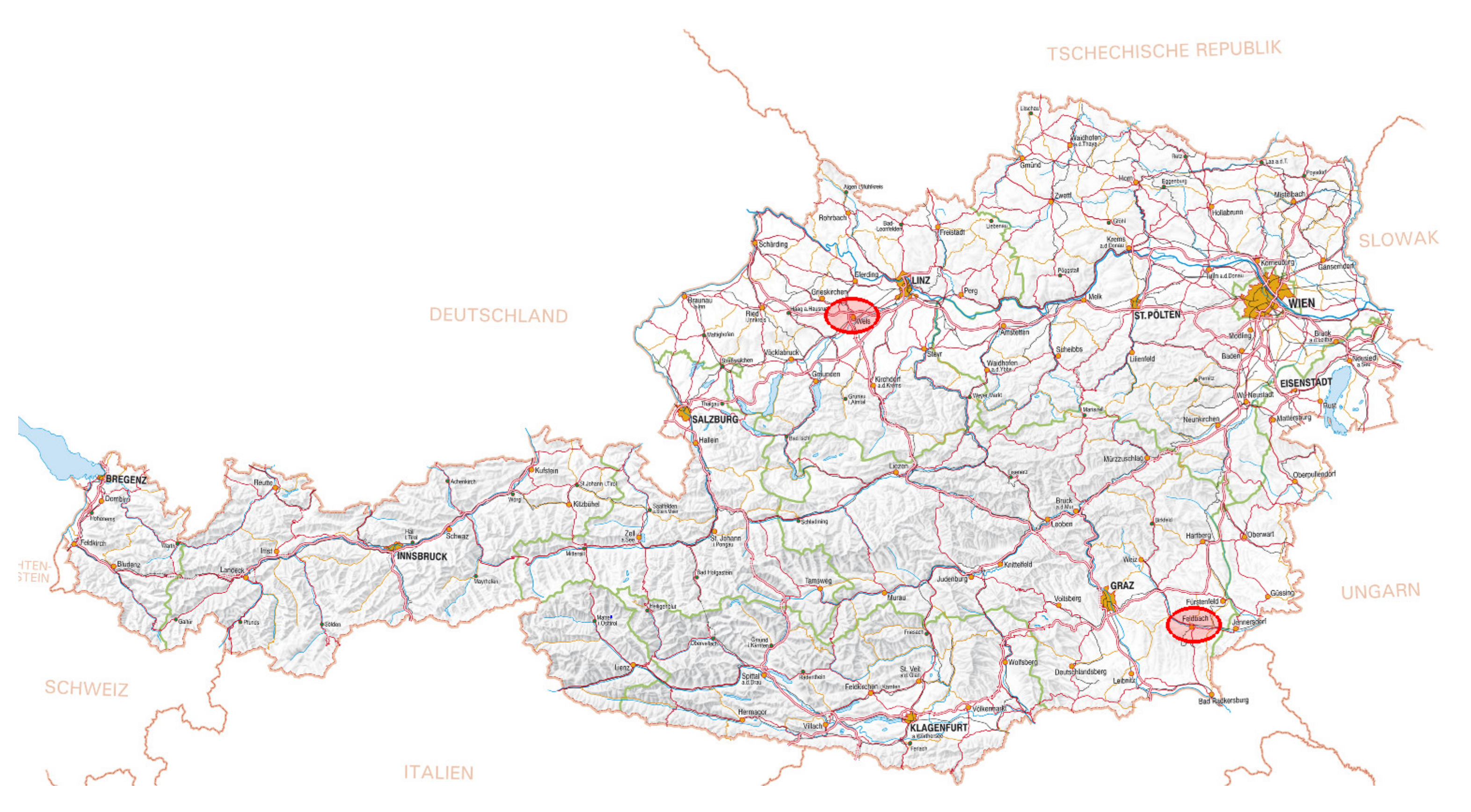
2. Materials and Methods
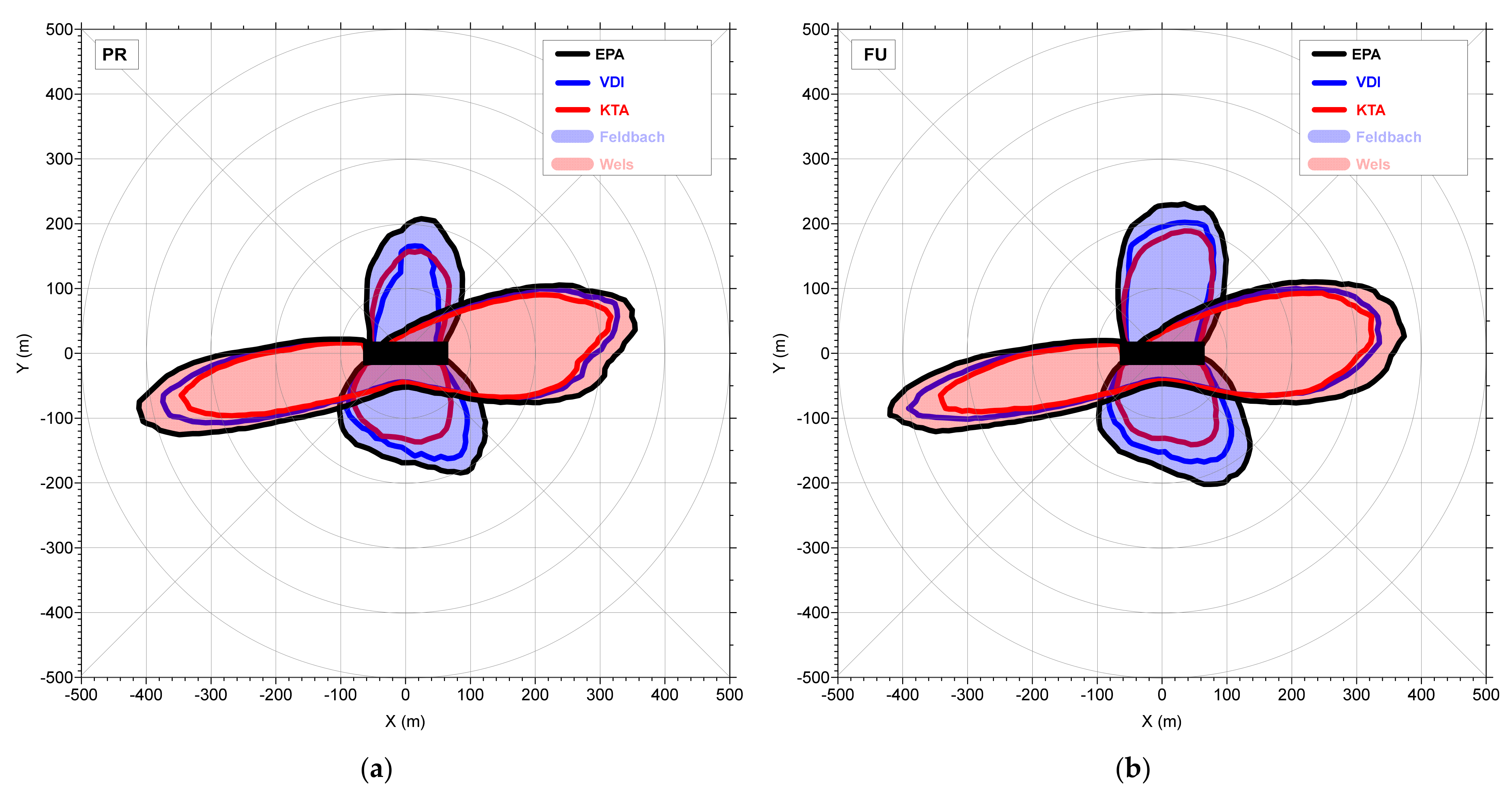
The two focus regions, Upper Austria north of the Alpine chain (centred around Wels, 48.16° N, 14.07° E) (Figure 1)and South-Eastern Styria (centred around Feldbach, 46.95° N, 15.88° E), are located within class Cfb (warm temperature, fully humid, warm summers) following the climate classification of Köppen and Geiger [6]. Instead of single sites, regions were chosen for the simulations, representative for livestock farming in Austria. The average meteorological conditions of the two regions are different: whereas the area around Wels north of the main Alpine chain is windy and humid, the focus region Feldbach south of the main Alpine chain is slightly more influenced by the Mediterranean and the Eastern European climate. For this investigation, meteorological parameters were needed which were derived from regional dynamical climate model output. With respect to the observed temperature, a so-called reference year was constructed from model output of a COSMO-CLM [7] simulation for the time period 1981–2010 covering the Alpine Region with a spatial resolution of 9 km forced by ERA-interim reanalysis data [8]. Simulated annual time series of the meteorological parameters air temperature, wind direction, wind speed, radiation balance, global radiation and total cloud cover were provided for the two regions of investigation on an hourly basis representative for the climate period 1981–2010. For the future climatic scenario, the climate change signal was derived from EURO-CORDEX regional climate model simulations for the mean temperature only, which was the most robust signal [9,10]. The climate change scenario was RCP4.5 which assumes an emission maximum in the middle of the century and a stabilisation of the CO2 concentration at the end of the century. The ensemble mean temperature change was added to the observed temperature, and a second reference year was derived from the regional-scale climate model simulations, which was representative for the future climate period of 2036–2065.
The dispersion model LASAT [11], which simulates the dispersion and the transport of a representative sample of tracer particles (in this case odorants) utilising a random walk process (Lagrangian simulation),was used to calculate separation distances. It computed the transport of passive trace substances in the lower atmosphere (up to heights of about 2000 m) on a local and regional scale (up to distances of about 150 km). LASAT is usually run with the Klug–Manier (K-M) stability scheme [12]. K-M classes were numbered from I to V and represented a simplified characterisation of the turbulence situation:
Dispersion categories V and IV comprise very unstable and unstable conditions, meaning good vertical mixing in the boundary layer. They did not occur during night-time. Category V occurred only between May and September.
Dispersion categories III/2 and III/1 are classified as neutral. III/2 occurred predominantly at daytime, III/1 predominantly at night-time and during sunrise and sunset. These categories are typical for cloudy and windy conditions.
Dispersion categories II and I comprise stable and very stable conditions, mostly, but not exclusively, at night.
In [5], cloudiness and radiation data, each in combination with wind speed, were used to determine stability classes. Here, in addition, the stability classification scheme proposed by the U.S. EPA (2000) [13] was applied, based on global radiation during daytime and the vertical temperature gradient at night. The scheme is depicted in Table 1, already transformed into K-M classes as required by the dispersion model LASAT. For completeness, the two other schemes are summarised in Table 2 and Table 3, taken from [5]. The six Pasquill stability classes A, B, C, D, E and F were assigned to K-M classes as follows: A … V, B … IV, C … III/2, D … III/1, E … II, F … I.
The source term data used for the presented LASAT model runs are summarised in Table 4. The odour emission rate and the odour concentration were given in so-called European odour units (ouE). By definition, the amount of exposure at which 50% of the panellists cannot smell the odour but 50% can, is equal to 1 odour unit per cubic metre. The source is assumed non-buoyant, i.e., the effective stack height is equal to the physical stack height. The source was a livestock building, 3 m high, 120 m long and 30 m wide. Along the main axis of the building, 9 stacks were located, centred at the middle of the roof, with an equal distance of 13.3 m. Each stack had a volume flow rate of 20,000 m3 h−1 and an odour emission rate of 1500ouEs−1.The total emission rate corresponded to 1930 fattening pigs, 113,000 broilers or 940 cattle [14]. Odorous substances were treated such as inert gases without modification during travel time. The odour emission of livestock buildings was composed of several tenths of substances. The main odorous substances causing odour sensation from pig houses are summarised by Zahn et al. [15]. Liu [16] gives the concentration and the odour threshold concentration for chemical substances which can be expected in pig houses. The following chemical substances were identified as potentially important odorant substances in pig odour with growing molar mass: ammonia, hydrogen sulphide, methanethiol, trimethylamine, propanoic acid, 2,3-butanedione, butanoic acid, pentanoic acid, 3-methylbutanoic acid, 4-methylphenol and 3-methyl-1H-indole. The source term data of Table 4 are very typical for Austrian livestock units and assumed constant over time; this assumption is discussed in Section 4.
Separation distances were calculated for the odour impact criteria defined in [17], namely, exceedance probabilities of 10% for pure residential and 15% for commercial/industrial and agriculturally dominated areas, each in combination with a preselected odour concentration threshold of 1ouEm³.
Usually, hourly mean values of concentrations were simulated by a dispersion model. Thus, a transformation of the hourly mean values calculated by the model to short-term concentrations relevant for human odour perception was necessary. The short-term peak concentrations were obtained via a peak-to-mean approach depending on atmospheric stability; the resulting site-independent peak-to-mean attenuation curves are shown in Figure 1 in [5]. For unstable conditions (classes V and IV), the peak-to-mean factors, starting at rather high values of about 10 near the source, rapidly approached 1 at about 100 m from the source. This is in agreement with the premise that vertical turbulent mixing can lead to short periods of local high ground-level concentrations, whereas the ambient mean concentrations were low. For neutral conditions (classes III/2 and III/1), the decrease in the peak-to-mean ratio was more gradual with increasing distance, because vertical mixing was reduced and horizontal diffusion was dominating the dispersion process. The peak-to-mean ratio in 100 m was then between 2 and 4. For stable conditions (classes II and I), the peak-to-mean ratio exceeded 2 only near the source. Stability class III/2 (“neutral”) gave the largest peak-to-mean factor for all distances between 100 and 500 m. In [18], the approach was described in detail; in [5], a shortened description was provided.

3. Results

3.1. Stability Classes

Here, only the parameters needed to determine EPA stability classes were presented, apart from the wind data already shown in [5]. The average daily course of global radiation was as expected (Figure 2): daytime values were on average culminating around noon at approx. 400 Wm−2 at both sites. The maximum values at Feldbach were slightly higher than at Wels because the south-alpine site was positioned further south and it was less cloudy and windy than the area around Wels. Only at Feldbach, a slight increase in global radiation around noon was calculated for the future climate, whereas no changes were shown for Wels. By definition, global radiation was zero during night-time.
To further confirm that the climate model data were consistent with expectations, seasonal variations in global radiation for Feldbach and Wels in the present climate are depicted in Figure 3. Feldbach showed especially higher noon values than Wels during the winter months. This was expected because the flatland site in Wels experiences more cloudiness and fog during winter than Feldbach. Similar results were obtained for the future climate period (not shown).
For both climate scenarios, daytime vertical temperature gradients were on average super-adiabatic (Figure 4), which is impossible in the free atmosphere. Day–night differences were more pronounced in Feldbach than in Wels caused by the lower winds and clearer skies at the former. Only at Feldbach, a decrease in the positive and increase in the negative temperature gradients were calculated for the future climate, whereas no changes at Wels occurred. The vertical temperature gradient was used only at night to determine stability classes (Table 1) when the data from the regional dynamical climate model output delivered plausible values.
The consistency of the climate data and the regional differences were further confirmed by Figure 5, which showed the dependence of the vertical temperature gradient on cloud amount at both sites in the present climate. As expected, Feldbach showed a larger variation in nocturnal temperature gradients than Wels, mainly due to the prevalent calm wind conditions at night. Wels, on the contrary, showed less variation during night-time, but a larger variation during daytime. On cloudy days, the daytime course was strongly reduced and lay almost in the expected daily range, with only a slight superadiabatic lapse rate during noon hours. Again, very similar features will occur in the future climate period (not shown).
In Figure 6, the EPA stability classes were grouped from very stable (class I) to very unstable (class V). There were systematic differences in the distribution of stability classes at both sites. At Wels, in the present scenario, class III/1 with more than 50% occurred most frequently (neutral at night). Class I showed a frequency of less than 20%, classes II, III/2 and IV around 10%. The very unstable class V occurred very seldom. In the future, stability class I will occur slightly more frequent, with an increase of about 2%. Class III/1 will occur slightly less frequent, whereas almost no changes were seen for the other classes.
Feldbach was generally characterised by more stable and unstable situations and less neutral conditions, compared to Wels. Classes I and III/1 showed frequencies of 30% and slightly more. For classes II, III/2 and IV, similar frequencies of about 10% were obtained. Comparing the present and the future scenario, the share for stability classes I and IV will be slightly reduced and that for class III/1 slightly increased. Almost no changes occurred for the other stability classes.
For comparison and to facilitate reading, the results for the other two methods (use of cloudiness data and radiation balance) presented in [2] are displayed in Figure 7. Compared to the results for the EPA method (Figure 5), the two other methods showed a much lower occurrence of class III/1, at both sites. Especially when using the KTA method (Figure 7b), a larger abundance for class I was obtained, at both sites. Using different methods to determine atmospheric stability, differences in the frequency distributions of the stability classes hadto be expected [4]. The choice of the method used will mostly depend on the available data; for the current investigation, data were available to apply three different methods to determine atmospheric stability. The resultant effect on the separation distances is shown in Section 3.2.

3.2. Separation Distances

In Figure 8 and Figure 9, the separation distances for the two selected protection levels determined by the EPA stability method were compared to those delineated from the VDI and the KTA methods [5]. They were calculated for two odour impact criteria according to [15], namely, a threshold of 1ouE m−3 and exceedance probabilities of 10% for pure residential areas (Figure 8) and 15% for commercial/industrial and agriculturally dominated areas (Figure 9).The separation distances were shown as isopleths, encompassing the area of exceedance of the given thresholds. An increase in (tolerated) exceedance probability reduced the affected area; a limit value of 15% (Figure 9 was, thus, more unfavourable for residents than a limit value of 10% (a higher level of protection, Figure 8). The black rectangle in the middle of all charts is the livestock building. The area displayed was 1000 × 1000 m2, with the odour source in the centre. The black lines depict separation distances obtained by the EPA method, the blue lines those of the VDI method and the red lines those of the KTA method. The affected area in the region centred around Wels is shown in red, the affected area in the region centred around Feldbach in blue. The spatial resolution of the separation distances was 5 m.
The addition of the EPA separation distances did not change the basic findings discussed in [5], i.e., the generally larger separation distances at Wels compared to Feldbach. This was due to the larger wind speeds and the more frequent neutral stability conditions found at Wels. For both the present and the future climate scenario, for both protection levels and at both sites, the EPA method delivered larger separation distances than the other methods. The increase was largest in Feldbach, in the present climate towards the north, in the future climate towards the south-east, and amounted to about 40 m. At Wels, the increase was larger for the lower protection level (Figure 9). At both sites, separation distances determined by the EPA method for the main wind directions will slightly increase in the future. This increase in separation distances means that a larger area might be affected by odour annoyance due to climate change, even if the emissions from the respective site were assumed unchanged. Compared to the other two stability classification schemes, the EPA method delivered the largest area of neighbourhood protection.

4. Discussion and Conclusions

As demonstrated in Figure 8 and Figure 9, separation distances showed variations, in this case depending on the used meteorological input data. In the presented scenarios, the differences resulted primarily from variations in the frequency distributions of stability classes (Figure 6 and Figure 7). The EPA method (Table 1) generally delivered the largest separation distances because the abundance of neutral stability classes was largest, associated with the highest peak-to-mean factors [5]. This result was valid at both sites despite the very different orographic and meteorological conditions and for both climate scenarios. At the flatland site in Wels, separation distances were generally larger than at Feldbach, due to the on average higher wind speeds and the more frequent neutral atmospheric stratification. At Feldbach, in addition, a very special result showed up, already discussed in [5]: If a frequency of exceedancesof 15% was tolerated, no separation distance north of the livestock unit was determined in the present climate with the cloudiness method (Figure 9a). This was explained by the combination of relatively low wind speeds and low frequencies of neutral stability (Figure 7a) which were associated with the highest peak-to-mean factor.
Earlier investigations revealed a similarly large variety of areas affected by odour annoyance under different orographic and climatic conditions. In [4], it could be demonstrated that separation distances for a site in a narrow valley can be larger than those in the flatlands. Although the flatland site was characterised by higher wind speeds, lower turbulence and somewhat larger peak-to-mean factors than the valley site, the larger separation distances there resulted from a frequent combination of the along-valley channelling of the flow in combination with frequent stable conditions causing higher odour concentrations and leading to the enhanced separation distances. The specific on-site meteorological conditions, thus can, exert a profound and sometimes surprising influence on resulting separation distances. An investigation in [18], carried out at an Austrian flatland site, compared separation distances obtained with a Gaussian and a Lagrangian model using site-specific peak-to-mean ratios and factor four used independent of the distance from the source and the meteorological conditions [12]. A continuous increase in separation distances from the Gaussian over the Lagrangian model to using the factor four (for both models) was found. The separation distances resulting from the factor four were judged unrealistically large, especially in the main wind directions and at sites where low wind speeds and/or stable dispersion categories are prevalent.
In the present investigation, the regional dynamical climate model output instead of observations at meteorological stations was used to determine separation distances (Section 2). The extracted data allowed the use of three different methods to determine stability classes (Table 1, Table 2 and Table 3). The frequency distributions of stability classes varied from method to method, but generally met the expected range and tendency. In particular, the dominance of neutral stability classes at flatland sites versus the large abundance of stable and unstable classes at valley or basin sites was confirmed also by the use of the model data. The fact that the climate model data delivered unrealistic superadiabatic vertical temperature gradients during daytime at both sites (Figure 4 and Figure 5) was not relevant for the determination of EPA stability classes, as the vertical temperature gradient was used only at night-time (Table 1) when it showed a realistic range of values. The range of separation distances also agreed well with those derived from meteorological data (compare the range of distances in [4,18] with Figure 8 and Figure 9 in this work).
Separation distances in this investigation were calculated assuming constant emissions over time (annual mean value), although odour emissions were often characterised by temporal variability [19,20]. Overall, the results in these papers indicate that the common practice of assuming a constant value for the odour emission can underestimate the separation distances to avoid annoyance, as compared to more realistic scenarios with hourly varying emission rates. Such an underestimation was observed to be more pronounced in the prevailing wind directions. The results also showed that the lower the selected exceedance probability of a specific odour impact criterion, the larger the separation distance underestimation. We selected odour impact criteria with exceedance probabilities of 10 and 15%, which meant that the impact of the assumption of a constant odour emission was small.
The presented results as well as previous investigations revealed the dependency of local-scale dispersion simulations on the meteorological input as a major source of model uncertainty. From model evaluation studies undertaken in the framework of EU-COST (see, e.g., [21,22,23,24]), the so-called fitness-for-purpose concept evolved, meaning that the type of model and source of data most apt for the purpose of an investigation should have been used. In the case of a complex terrain, for example, the use of a Lagrangian model is to be preferred over a Gaussian one. With data from three-axis ultrasonic anemometers, site-specific peak-to-mean attenuation curves can be obtained, and wind and stability information are obtained from one instrument [4,18]. If available, such data are preferred over data from conventional (mostly semi-automatic) meteorological stations. Even then, a range of results are obtained, whenever different models or datasets are used.
This investigation showed that, due by climate change, current protection areas might not be sufficient in the future. The Feldbach case revealed that separation distances would have to be increased by approx. 50 m, especially in the main wind directions. In addition, climate change will likely also lead to an increase in emissions, caused, e.g., by the increased animal activity due to heat stress [25], probably further increasing separation distances. In contrast to Feldbach, however, the calculations for Wels showed only marginal changes of the affected area in the future. The influence of climate change on odour dispersion has to, therefore, be investigated on a case-by-case basis, best using the methodology presented in the current work.
If the focus of an investigation lies on neighbourhood protection, a stricter odour impact criterion should be used, leading to larger separation distances in terms of a worst case scenario. For the current investigation, the EPA method was preferred over the VDI and KTA schemes, as it delivered generally larger separation distances. As the climate conditions at the two sites were very different, this outcome can be generalized.

Author Contributions

Conceptualization, writing—original draft preparation, M.P.; methodology, M.P., K.B.-S., I.A. and G.S.; software analysis and validation, W.K. and K.A.; writing—review and editing, M.P., G.S., K.B.-S. and I.A.; visualization, W.K. All authors have read and agreed to the published version of the manuscript.

Funding

The project PiPoCooL “Climate change and future pig and poultry production: implications for animal health, welfare, performance, environment and economic consequences” was funded by the Austrian Climate and Energy Fund in the framework of the Austrian Climate Research Program(ACRP8–PiPoCooL–KR15AC8K12646).

Data Availability Statement

The CORDEX (Coordinated Regional Climate Downscaling Experiment)data are available from the Earth System Grid Federation (ESGF), https://cordex.org/data-access/esgf/, latest access date: 31 August 2016. The data presented in this study are available on request from the corresponding author.

Acknowledgments

We acknowledge the World Climate Research Programme’s Working Group on Regional Climate, and the Working Group on Coupled Modelling, former coordinating body of CORDEX, a responsible panel for CMIP5. We also thank the climate modelling groups for producing and making available their model output. We also acknowledge the Earth System Grid Federation infrastructure, an international effort led by the U.S. Department of Energy’s Program for Climate Model Diagnosis and Intercomparison, the European Network for Earth System Modelling and other partners in the Global Organisation for Earth System Science Portals (GO-ESSP).

Conflicts of Interest

The authors declare no conflict of interest.

References

  1. Leelőssy, Á.; Molnár, F., Jr.; Izsák, F.; Havasi, Á.; Lagzi, I.; Mészáros, R. Dispersion modeling of air pollutants in the atmosphere: A review. Cent. Euro. J. Geosci. 2014, 6, 257–278. [Google Scholar] [CrossRef]
  2. Brancher, M.; Griffiths, K.D.; Franco, D.; De MeloLisboa, H. A review of odour impact criteria in selected countries around the world. Chemosphere 2017, 168, 1531–1570. [Google Scholar] [CrossRef] [PubMed]
  3. Sommer-Quabach, E.; Piringer, M.; Petz, E.; Schauberger, G. Comparability of separation distances between odour sources and residential areas determined by various national odour impact criteria. Atmos. Environ. 2014, 95, 20–28. [Google Scholar] [CrossRef]
  4. Piringer, M.; Knauder, W.; Petz, E.; Schauberger, G. Factors influencing separation distances against odour annoyance calculated by Gaussian and Langrangian dispersion models. Atmos. Environ. 2016, 140, 69–83. [Google Scholar] [CrossRef]
  5. Piringer, M.; Knauder, W.; Anders, I.; Andre, K.; Zollitsch, W.; Hörtenhuber, S.J.; Baumgartner, J.; Niebuhr, K.; Hennig-Pauka, I.; Schönhart, M.; et al. Climate change impact on the dispersion of airborne emissions and the resulting separation distances to avoid odour annoyance. Atmos. Environ. X 2019, 2, 100021. [Google Scholar] [CrossRef]
  6. Kottek, M.; Grieser, J.; Beck, C.; Rudolf, B.; Rubel, F. World map of the Köppen-Geiger climate classification updated. Meteorol. Z. 2006, 15, 259–263. [Google Scholar] [CrossRef]
  7. Rockel, B.; Will, A.; Hense, A. The Regional Climate Model COSMO-CLM (CCLM). Meteorol. Z. 2008, 17, 347–348. [Google Scholar] [CrossRef]
  8. Dee, D.P.; Uppala, S.M.; Simmons, A.J.; Berrisford, P.; Poli, P.; Kobayashi, S.; Andrae, U.; Balmaseda, M.A.; Balsamo, G.; Bauer, P.; et al. The ERA-Interim reanalysis: Configuration and performance of the data assimilation system. Q. J. R. Meteorol. Soc. 2011, 137, 553–597. [Google Scholar] [CrossRef]
  9. Smiatek, G.; Kunstmann, H.; Senatore, A. EURO-CORDEX regional climate model analysis for the Greater Alpine Region: Performance and expected future change. J. Geophys. Res. Atmos. 2016, 121, 7710–7728. [Google Scholar] [CrossRef] [Green Version]
  10. Jacob, D.; Petersen, J.; Eggert, B.; Alias, A.; Bøssing Christensen, O.; Bouwer, L.M.; Braun, A.; Colette, A.; Déqué, M.; Georgievski, G.; et al. EURO-CORDEX: New high-resolution climate change projections for European impact research. Reg. Environ. Chang. 2014, 14, 563. [Google Scholar] [CrossRef]
  11. Janicke Consulting. Dispersion Model LASAT Version 3.4, Reference Book; Janicke Consulting Environmental Physics: Überlingen, Germany, 2019. [Google Scholar]
  12. Bundesministerium für Umwelt, Naturschutz und Reaktorsicherheit. Erste Allgemeine Verwaltungsvorschrift zum Bundes–Immissionsschutzgesetz (Technische Anleitung zur Reinhaltung der Luft—TA Luft); Bundesministerium für Umwelt, Naturschutz und Reaktorsicherheit: Berlin, Germany, 2002.
  13. EPA. Meteorological Monitoring Guidance for Regulatory Modeling Applications; United States Environmental Protection Agency (EPA): Washington, DC, USA, 2000.
  14. VDI. Emissions and Immissions from Animal Husbandry—Housing Systems and Emissions—Pigs, Cattle, Poultry, Horses; VDI 3894 Part 1; Verein Deutscher Ingenieure, VDI Verlag: Düsseldorf, Germany, 2011. [Google Scholar]
  15. Zahn, J.A.; DiSpirito, A.A.; Do, Y.S.; Brooks, B.E.; Cooper, E.E.; Hatfield, J.L. Correlation of human olfactory responses to airborne concentrations of malodorous volatile organic compounds emitted from swine effluent. J. Environ. Qual. 2001, 30, 624–634. [Google Scholar] [CrossRef] [PubMed] [Green Version]
  16. Liu, D. Application of PTR-MS for Optimization of Odour Removal from Intensive Pig Production with Emphasis on Biofiltration; Department of Engineering—Biological and Chemical Engineering, Aarhus University: Aarhus, Denmark, 2013. [Google Scholar]
  17. GOAA. Guideline on Odour in Ambient Air. In Detection and Assessment of Odour in Ambient Air, 2nd ed.; GOAA: Berlin, Germany, 2008. [Google Scholar]
  18. Piringer, M.; Knauder, W.; Petz, E.; Schauberger, G. A comparison of separation distances against odour annoyance calculated with two models. Atmos. Environ. 2015, 116, 22–35. [Google Scholar] [CrossRef]
  19. Brancher, M.; Knauder, W.; Piringer, M.; Schauberger, G. Temporal variability in odour emissions: To what extent this matters for the assessment of annoyance using dispersion modelling. Atmos. Environ. X 2020, 5, 100054. [Google Scholar] [CrossRef]
  20. Schauberger, G.; Piringer, M.; Heber, A.J. Odour emission scenarios for fattening pigs as input for dispersion models: A step from an annual mean value to time series. Agric. Ecosyst. Environ. 2014, 93, 108–116. [Google Scholar] [CrossRef]
  21. Baumann-Stanzer, K.; Piringer, M.; Polreich, E.; Hirtl, M.; Petz, E.; Bügelmayer, M. User experience with model validation exercises. Croat. Meteorol. J. 2008, 43, 52–56. [Google Scholar]
  22. Piringer, M.; Baumann-Stanzer, K. Selected results of a model validation exercise. Adv. Sci. Res. 2009, 3, 13–16. [Google Scholar] [CrossRef] [Green Version]
  23. Baumann-Stanzer, K.; Piringer, M. Validation of regulatory micro-scale air quality models: Modeling odour dispersion and built-up areas. World Rev. Sci. Technol. Sustain. Dev. 2011, 8, 203–213. [Google Scholar] [CrossRef]
  24. Di Sabatino, S.; Buccolieri, R.; Olesen, H.R.; Ketzel, M.; Berkowicz, R.; Franke, J.; Schatzmann, M.; Schlünzen, K.H.; Leitl, B.; Britter, R.; et al. COST 732 in practice: The MUST model evaluation exercise. Int. J. Environ. Pollut. 2011, 44, 403–418. [Google Scholar] [CrossRef] [Green Version]
  25. Schauberger, G.; Hennig-Pauka, I.; Zollitsch, W.; Hörtenhuber, S.J.; Baumgartner, J.; Niebuhr, K.; Piringer, M.; Knauder, W.; Anders, I.; Andre, K.; et al. Efficacy of adaptation measures to alleviate heat stress in confined livestock buildings in temperate climate zones. Biosyst. Eng. 2020, 200, 157–175. [Google Scholar] [CrossRef]
Figure 1. Map of Austria showing the two focus regions (red areas) Wels (in the north) and Feldbach (in the south-east).
Atmosphere 12 01149 g001
Figure 2. Annual mean of the daily course of global radiation for Feldbach and Wels (PR = present (1981–2010), FU = future (2036–2065)).
Atmosphere 12 01149 g002
Figure 3. Winter, summer and annual means of the daily course of global radiation for (a) Feldbach and (b) Wels; PR—present (1981–2010).
Atmosphere 12 01149 g003
Figure 4. Annual mean of the daily course of the vertical temperature gradient (K (100 m)1) for Feldbach and Wels (PR—present (1981–2010); FU—future (2036–2065)).
Atmosphere 12 01149 g004
Figure 5. Annual mean of the daily course of the vertical temperature gradient (K (100 m)1) for low cloud cover (orange line), high cloud cover (blue line) and all data (black line) for (a) Feldbach and (b) Wels; PR—present (1981–2010).
Atmosphere 12 01149 g005
Figure 6. Frequency distribution of EPA stability classes determined according to Table 1 at Feldbach and Wels (PR—present (1981–2010); FU—future (2036–2065)).
Atmosphere 12 01149 g006
Figure 7. Frequency distribution of stability classes determined by (a) cloudiness and wind speed (VDI method, Table 2) and (b) radiation balance and wind speed (KTA method, Table 3) at Feldbach and Wels (PR—present (1981–2010); FU—future (2036–2065)) (taken from [5]).
Atmosphere 12 01149 g007
Figure 8. Direction-dependent separation distances (m) for 10% exceedance probability (pure residential areas) at Feldbach and Wels, (a) for PR (present climate (1981–2010)) and (b) FU (future climate (2036–2065)); based on a combination of global radiation and the vertical temperature gradient (EPA), cloudiness (VDI) and radiation balance (KTA), each in combination with wind speed, to determine stability classes; the black rectangle is the livestock building.
Atmosphere 12 01149 g008
Figure 9. Direction-dependent separation distances (m) for 15% exceedance probability (commercial/industrial and agriculturally dominated areas) at Feldbach and Wels, (a) for PR (present climate (1981–2010)) and (b) FU (future climate (2036–2065)); based on a combination of global radiation and the vertical temperature gradient (EPA), cloudiness (VDI) and radiation balance (KTA), each in combination with wind speed, to determine stability classes; the black rectangle is the livestock building.
Atmosphere 12 01149 g009
Table 1. Scheme to determine U.S. EPA stability classes (transformed to K-M classes).
DAYTIME (Global Radiation ≥ 20 Wm−2)
Global Radiation (Wm−2)
Wind Speed (ms−1)≥925925–675675–175175–20
<2VVIVIII/1
2–2.9VIVIII/2III/1
3–4.9IVIVIII/2III/1
5–5.9III/2III/2III/1III/1
≥6III/2III/1III/1III/1
NIGHTTIME (Global Radiation < 20 Wm−2)
Vertical Temperature Gradient (K(100 m)−1)
Wind Speed (ms−1)<0≥0
<2III
2–2.9III/1II
≥3III/1III/1
Table 2. VDI scheme to determine Klug/Manier stability classes via cloudiness data (taken from [5]).
Wind Speed υ10 at 10 m Height (z0 = 0.1 m)Night-TimeDaytime
Total Cloud CoverTotal Cloud Cover
in ms−10/8 to 6/87/8 to 8/80/8 to 2/83/8 to 5/86/8 to 8/8
≤1.2IIIIVIVIV
1.3 to 2.3IIIIVIVIII/2
2.4 to 3.3IIIII/1IVIVIII/2
3.4 to 4.3III/1III/1IVIII/2III/2
≥4.4III/1III/1III/2III/1III/1
Table 3. KTA scheme to determine stability classes based on the radiation balance and the wind speed (taken from [5]).
Wind Speed υ10 at 10 m Height Radiation Balance in Wm−2
Limits of Categories
In ms−1A/BB/CC/DD/EE/F
0 to 0.921412560−2−9
1.0 to 1.921412660−4−13
2.0 to 2.930116260−6−21
3.0 to 3.940023263−12−34
4.0 to 4.949530567−28−55
5.0 to 5.937684−55
6.0 to 6.9450108
7.0 to 7.9150
8.0 to 9.9240
≥10.0All values category D
Example:
If the conditions 2.0 ms−1 ≤ u10 < 3.0 ms−1 and 162 Wm−2 ≥ radiation balance > 60 Wm−2 were fulfilled, then category C was used.
Table 4. Source term data for dispersion calculations.
Stack height(m)5.0
Stack diameter(m)1.88
Number of stacks 9
Outlet air velocity(ms−1)2.0
Volume flow rate(m3 h−1)180,000
Temperature(°C)0
Odour emission rate (ouEs−1)13,500
Concentration(ouEm−3)270
Publisher’s Note: MDPI stays neutral with regard to jurisdictional claims in published maps and institutional affiliations.

