
Analysis of Cooling and Heating Degree Days over Mexico in Present and Future Climate

 ,
,
Abstract
:1. Introduction
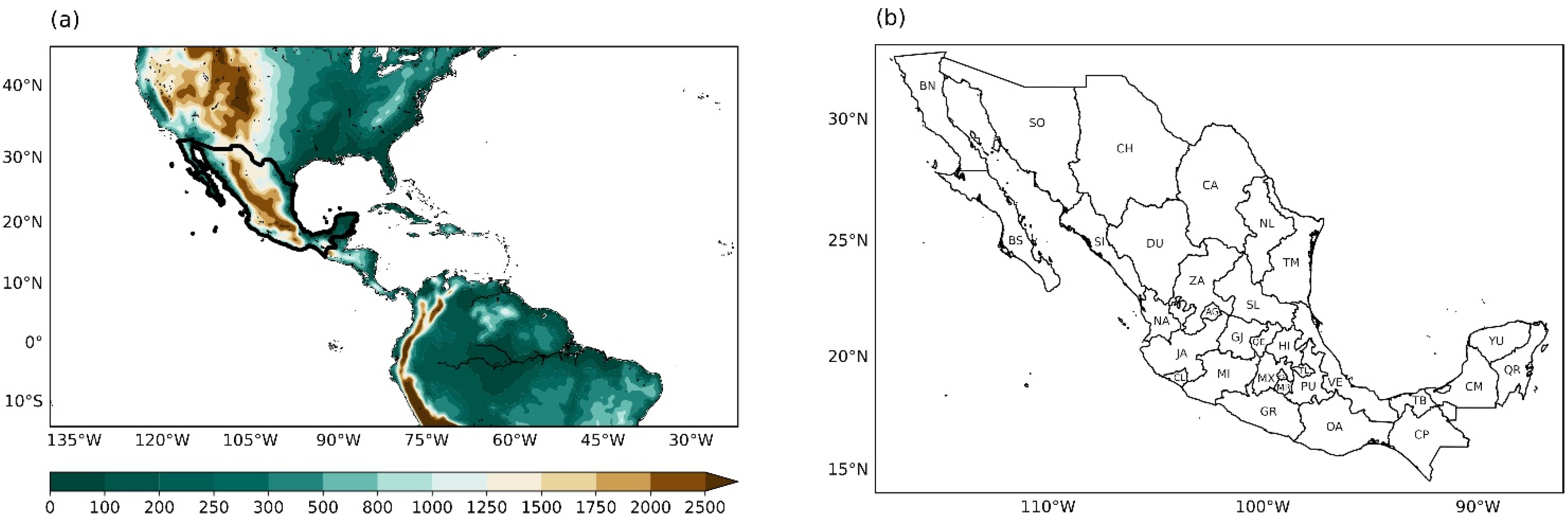
2. Materials and Methods
2.1. Model
Simulations
- Met Office Hadley Centre, Exeter, United Kingdom, MOHC-HadGEM2-ES, (M1),
- Max Planck Institute for Meteorology, Hamburg, Germany, MPI-M; M-MPI-ESM-LR, (M2),
- NOAA-Geophysical Fluid Dynamics Laboratory, Princeton University Forrestal Campus, USA, NOAA-GFDL-ESM2M, (M3).
2.2. Data
- (i)
- Livneh observational data-set gridded to a 1/16° (~6 km) resolution, that spans the entire country of Mexico, USA, and southern Canada for the period 1950–2013 ([31], ftp://192.12.137.7/pub/dcp/archive/OBS/livneh2014.1_16deg/, date of access: 1 June 2020),
- (ii)
- CPC Global Temperature data with 0.50° resolution for 1 January 1979 to present provided by the NOAA/OAR/ESRL PSL, Boulder, CO, USA, from their Web site at https://psl.noaa.gov/, date of access: 15 June 2020, and
- (iii)
- ERA5 reanalysis (spanning 1979 onwards) of the European Centre for Medium-Range Weather Forecast (ECMWF) at a horizontal resolution of 31 km ([32,33], https://cds.climate.copernicus.eu/cdsapp#!/home, date of access: 15 May 2020).
2.3. Cooling and Heating Degree Days
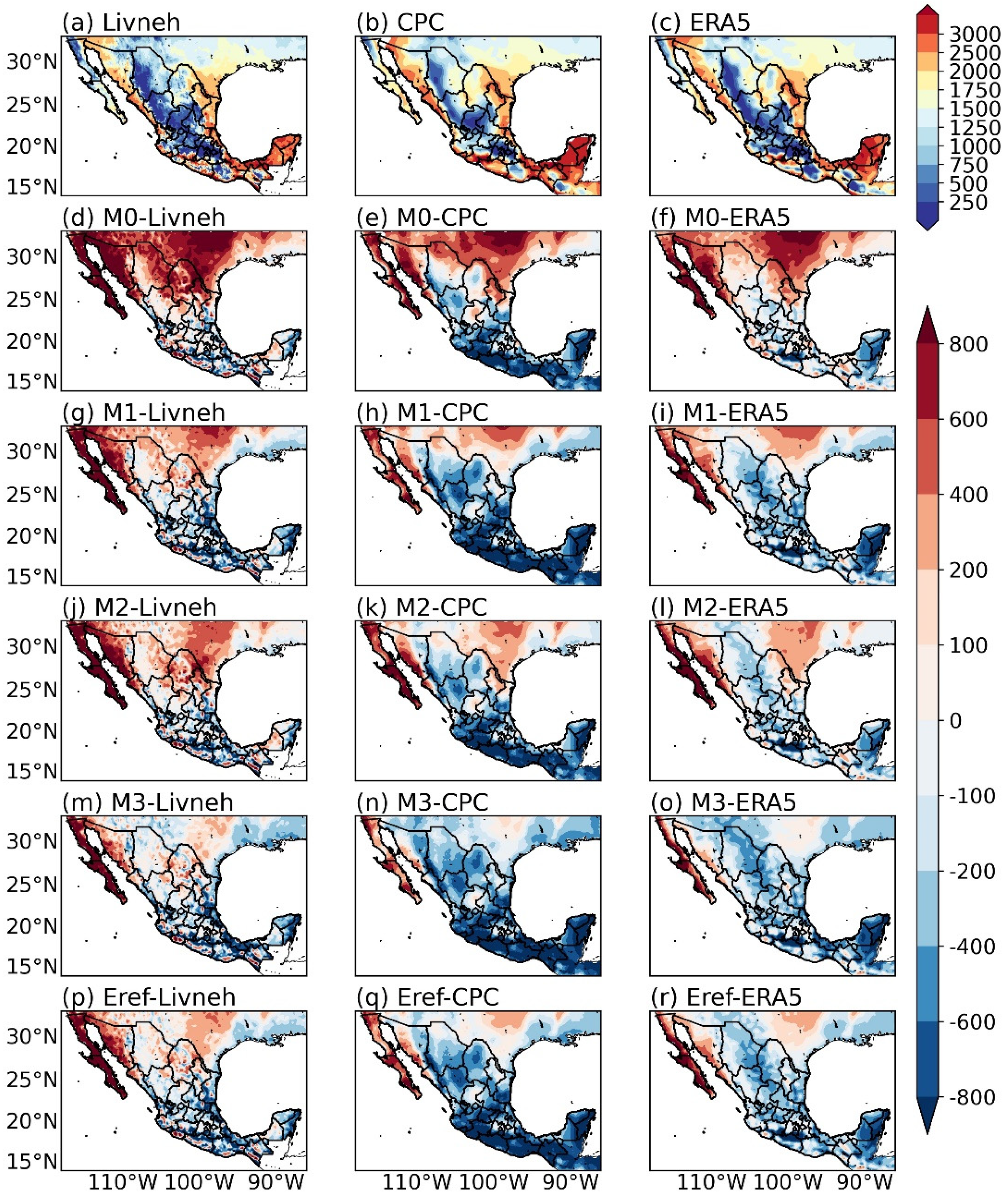
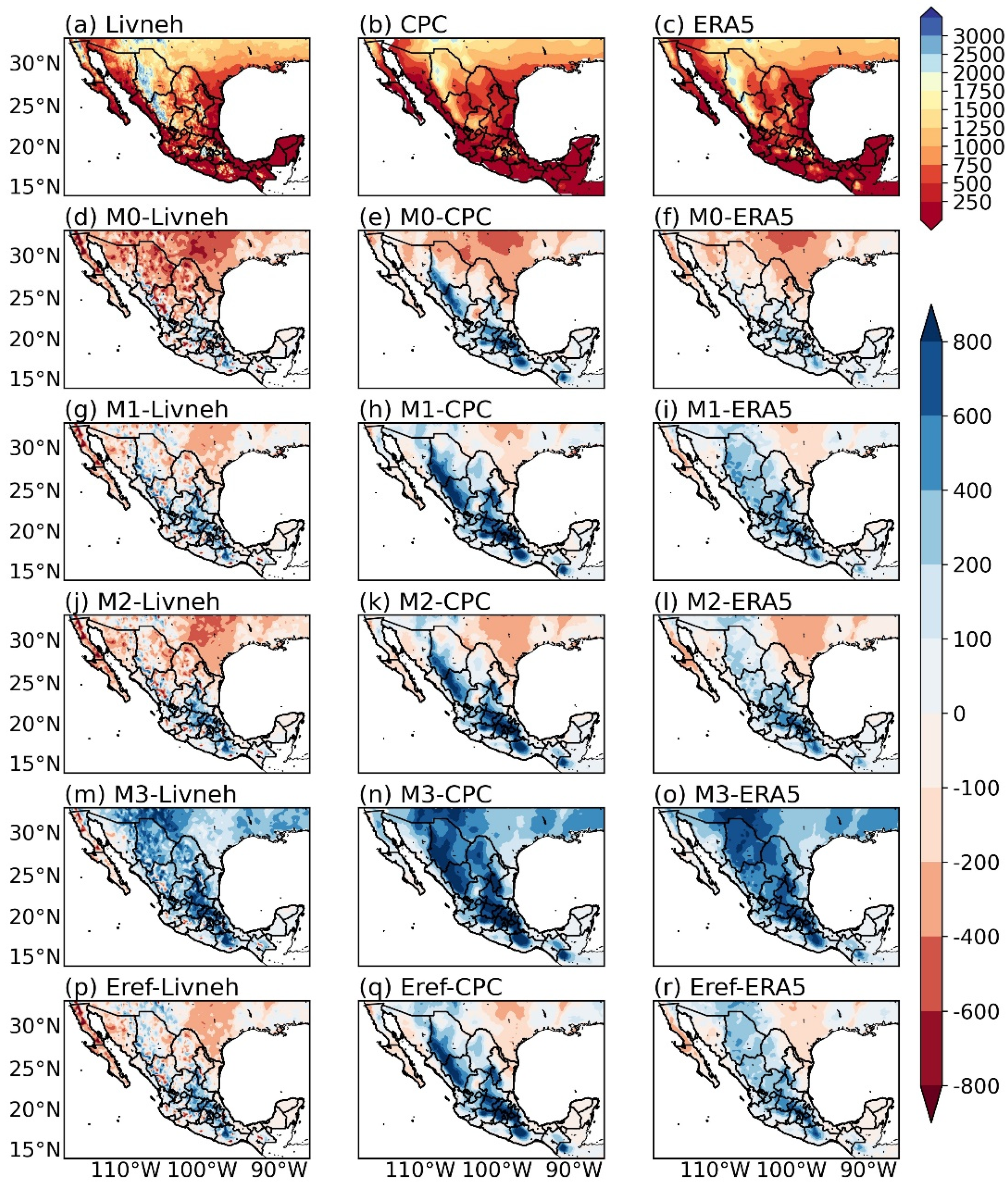
3. Results
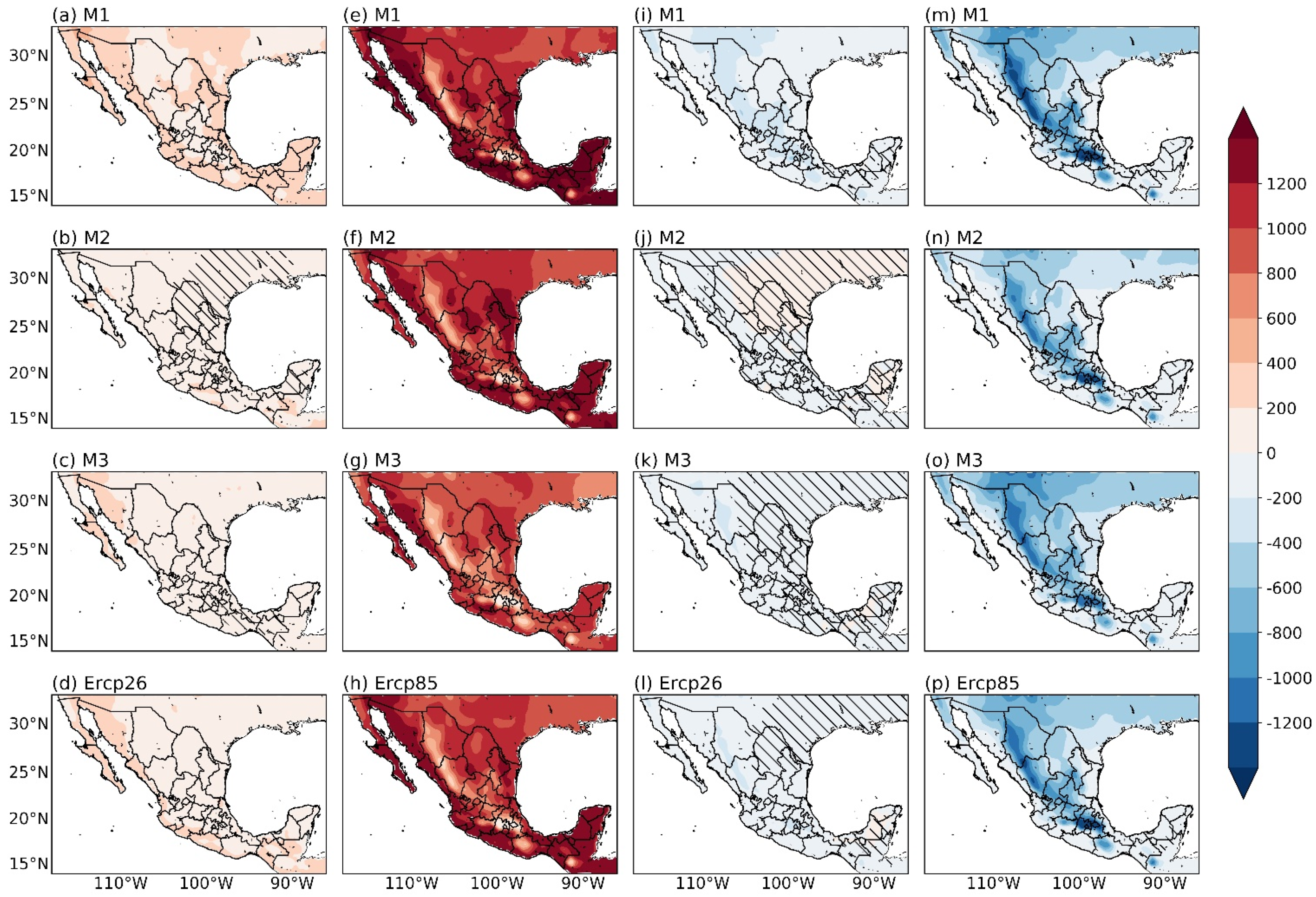
3.1. Reference Period
Cooling and Heating Degree Days
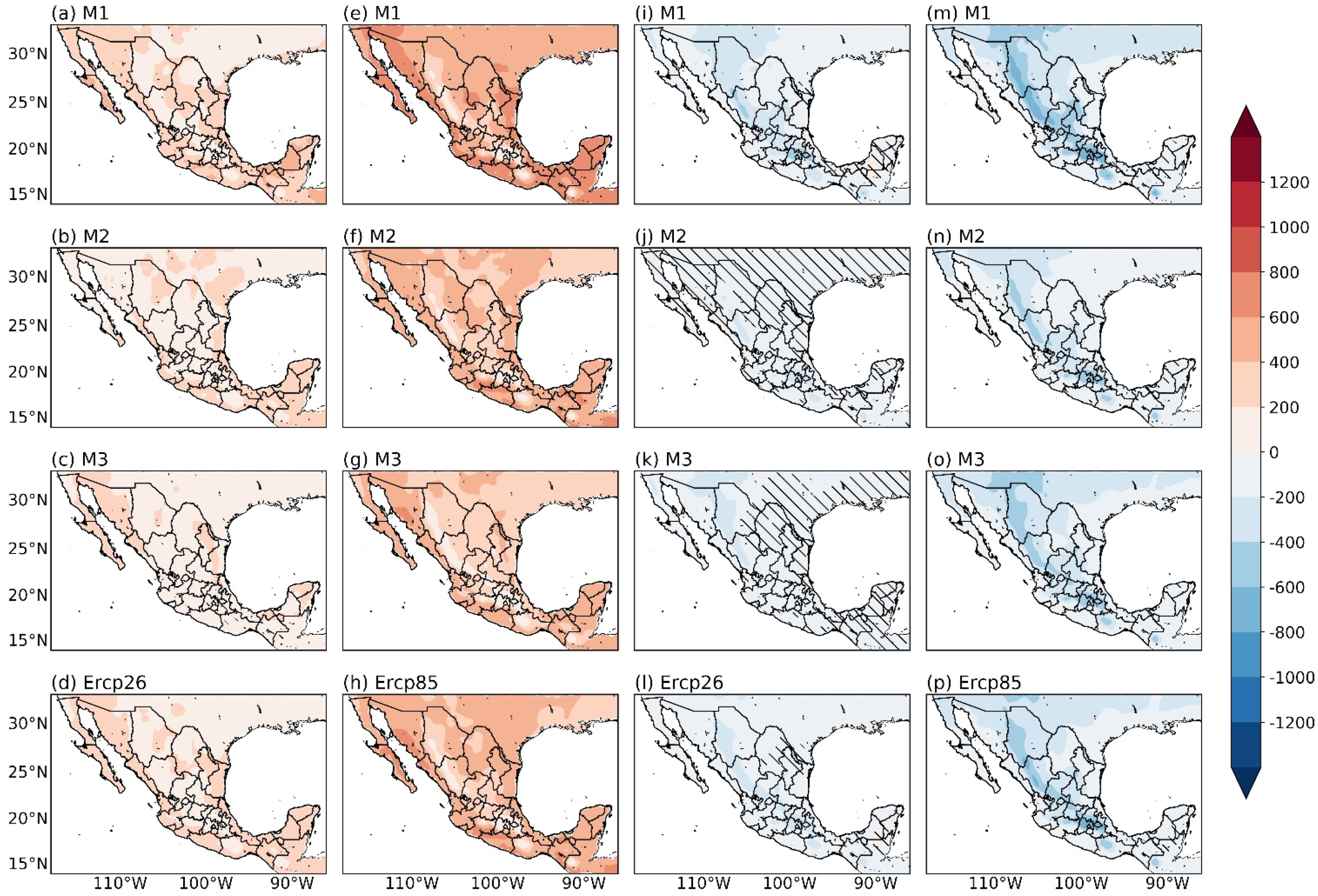
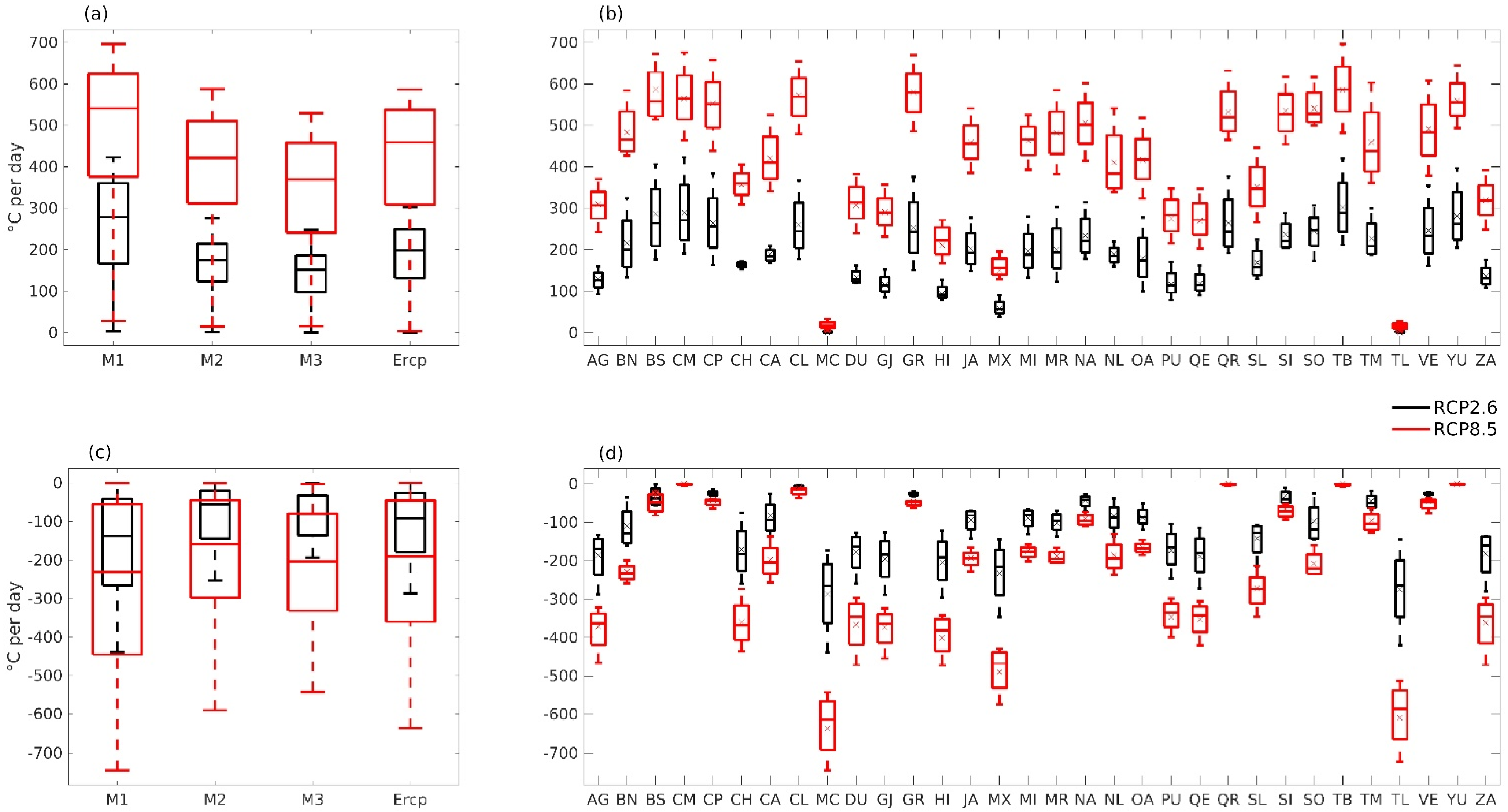
3.2. Future Period
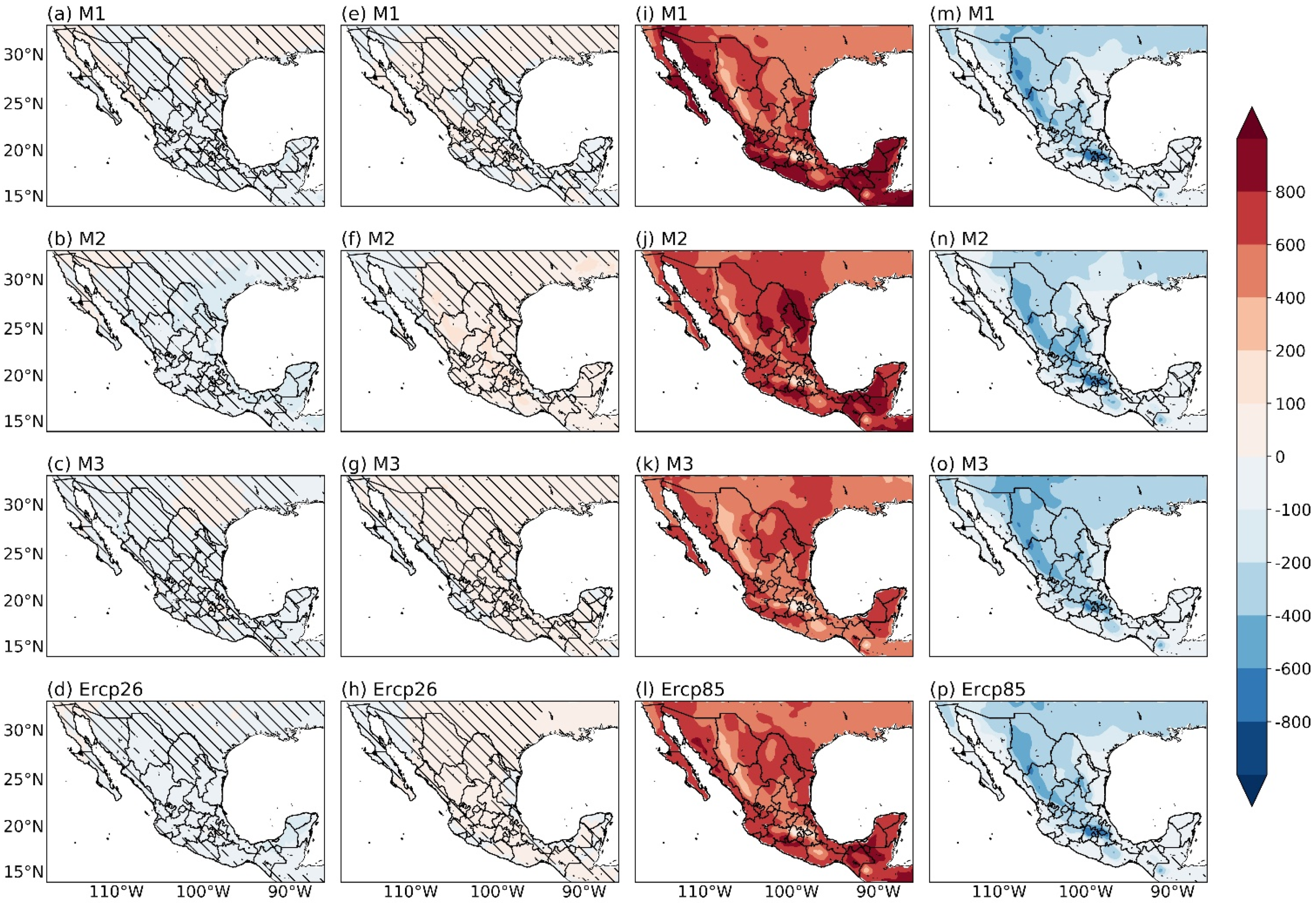
3.2.1. Near-Future (2041–2060)
Cooling and Heating Degree Days
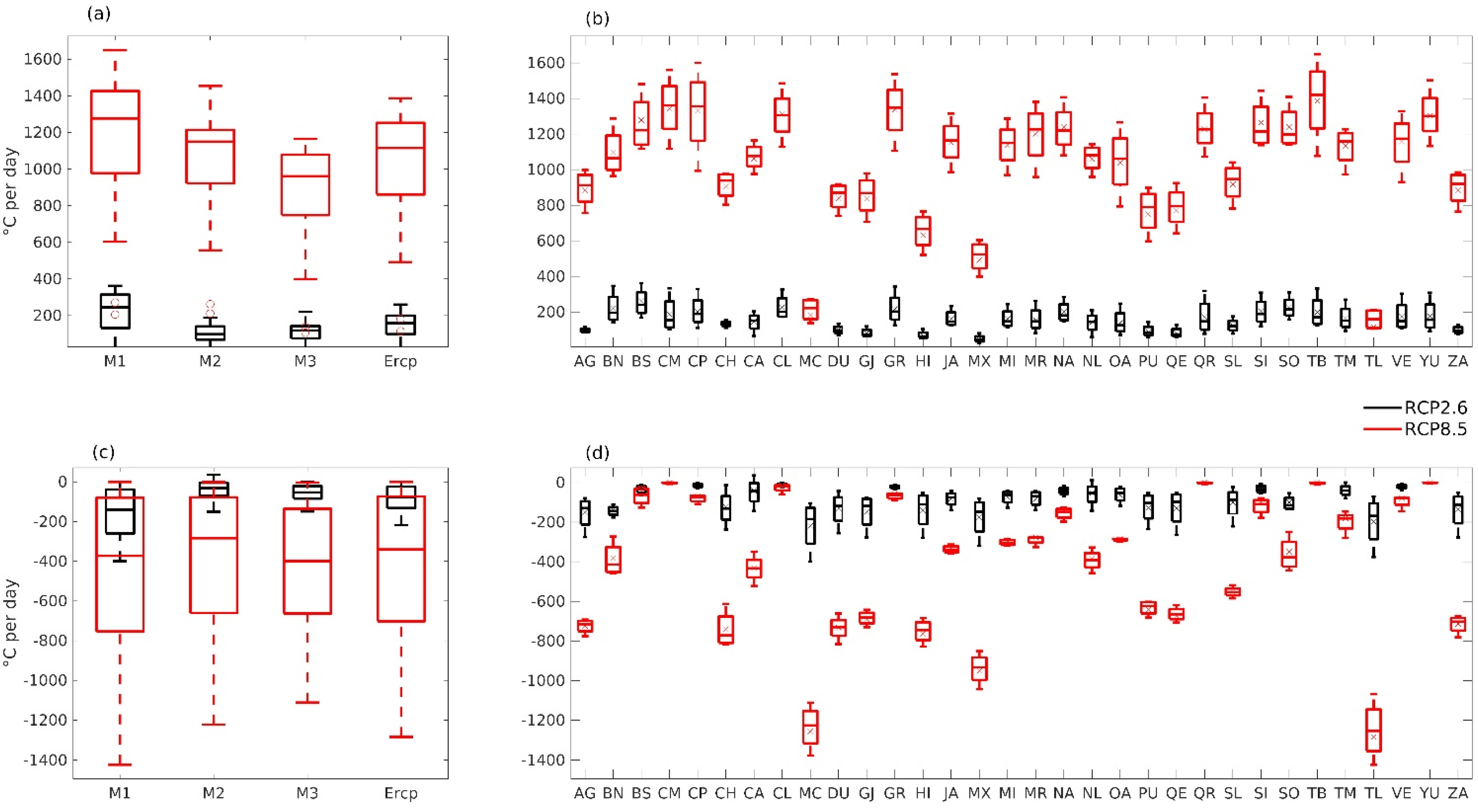
3.2.2. Far-Future (2080–2099)
Cooling and Heating Degree Days
4. Discussion
5. Conclusions
Supplementary Materials
Author Contributions
Funding
Institutional Review Board Statement
Informed Consent Statement
Data Availability Statement
Acknowledgments
Conflicts of Interest
References
- IPCC. Climate Change 2013: The physical science basis. In Contribution of Working Group I to the 5th Assessment Report of the Intergovernmental Panel on Climate Change; Stocker, T.F., Qin, D.H., Plattner, G.K., Tignor, M., Eds.; Cambridge University Press: Cambridge, UK, 2013. [Google Scholar]
- Giorgi, F. Climate change hot-spots. Geophys. Res. Lett. 2006, 33, L08707. [Google Scholar] [CrossRef]
- Şen, Z.; Kadioǧlu, M. Heating degree-days for arid regions. Energy 1998, 23, 1089–1094. [Google Scholar] [CrossRef]
- Kadioglu, M.; Şen, Z. Degree-Day Formulations and Application in Turkey. J. Appl. Meteorol. 1999, 38, 837–846. [Google Scholar] [CrossRef]
- Al-Hadhrami, L. Comprehensive review of cooling and heating degree days characteristics over Kingdom of Saudi Arabia. Renew. Sustain. Energy Rev. 2013, 27, 305–314. [Google Scholar] [CrossRef]
- Shi, Y.; Gao, X.; Xu, Y.; Giorgi, F.; Chen, D. Effects of climate change on heating and cooling degree days and potential energy demand in the household sector of China. Clim. Res. 2016, 67, 135–149. [Google Scholar] [CrossRef] [Green Version]
- Büyükalaca, O.; Bulut, H.; Yilmaz, T. Analysis of variable-base heating and cooling degree-days for Turkey. Appl. Energy 2001, 69, 269–283. [Google Scholar] [CrossRef] [Green Version]
- Spinoni, J.; Vogt, J.; Barbosa, P. European degree-day climatologies and trends for the period 1951–2011. Int. J. Climatol. 2015, 35, 25–36. [Google Scholar] [CrossRef] [Green Version]
- Mistry, M.N. Historical global gridded degree-days: A high-spatial resolution database of CDD and HDD. Geosci. Data J. 2019, 6, 214–221. [Google Scholar] [CrossRef] [Green Version]
- Christenson, M.; Manz, H.; Gyalistras, D. Climate warming impact on degree- days and building energy demand in Switzerland. Energy Convers. Manag. 2006, 47, 671–686. [Google Scholar] [CrossRef]
- Shi, Y.; Zhang, D.; Xu, Y.; Zhou, B. Changes of heating and cooling degree days over China in response to global warming of 1.5 °C, 2 °C, 3 °C and 4 °C. Adv. Clim. Chang. Res. 2018, 9, 192–200. [Google Scholar] [CrossRef]
- Coppola, E.; Raffaele, F.; Giorgi, F.; Giuliani, G.; Xuejie, G.; Ciarlo, J.M.; Sines, T.R.; Torres-Alavez, J.A.; Das, S.; di Sante, F.; et al. Climate hazard indices projections based on CORDEX-CORE, CMIP5 and CMIP6 ensemble. Clim. Dyn. 2021, 57, 1293–1383. [Google Scholar] [CrossRef]
- Peña-Gallardo, R.; Medina-Ríos, A.; Segundo-Ramírez, J. Analysis of the solar and wind energetic complementarity in Mexico. J. Clean. Prod. 2020, 268, 122323. [Google Scholar] [CrossRef]
- Cámara de Diputados México. Ley para el Aprovechamiento de Energías Renovables y el Financiamiento de la Transición Energética. D. Of. La Fed. 1-16. 2013. Available online: https://www.cre.gob.mx/documento/3870.pdf (accessed on 1 May 2020).
- Pérez-Denicia, E.; Fernández-Luqueño, F.; Vilariño-Ayala, D.; Montaño-Zetina, L.M.; Maldonado-López, L.A. Renewable energy sources for electricity generation in Mexico: A review. Renew. Sustain. Energy Rev. 2017, 78, 597–613. [Google Scholar] [CrossRef]
- Giorgi, F.; Jones, C.; Asrar, G.R. Addressing Climate Information Needs at the Regional Level: The CORDEX Framework. World Meteorol. Organ. Bull. 2009, 58, 175–183. [Google Scholar]
- Giorgi, F.; Coppola, E.; Solmon, F.; Mariotti, L.; Sylla, M.B.; Bi, X.; Elguindi, N.; Diro, G.T.; Nair, V.; Giuliani, G.; et al. RegCM4: Model description and preliminary tests over multiple CORDEX domains. Clim. Res. 2012, 52, 7–29. [Google Scholar] [CrossRef] [Green Version]
- Giorgi, F.; Gutowski, W.J. Regional dynamical downscaling and the cordex initiative. Annu. Rev. Environ. Resour. 2015, 40, 467–490. [Google Scholar] [CrossRef]
- Torres-Alavez, J.A.; Das, S.; Corrales-Suastegui, A.; Coppola, E.; Giorgi, F.; Raffaele, F.; Bukovsky, M.S.; Ashfaq, M.; Salinas, J.A.; Sines, T. Future projections in the climatology of global low-level jets from CORDEX-CORE simulations. Clim. Dyn. 2021, 57, 1551–1569. [Google Scholar] [CrossRef]
- Torres-Alavez, J.A.; Glazer, R.; Giorgi, F.; Coppola, E.; Gao, X.; Hodges, K.I.; Das, S.; Ashfaq, M.; Reale, M.; Sines, T. Future projections in tropical cyclone activity over multiple CORDEX domains from RegCM4 CORDEX-CORE simulations. Clim. Dyn. 2021, 57, 1507–1531. [Google Scholar] [CrossRef]
- Fuentes-Franco, R.; Coppola, E.; Giorgi, F.; Pavia, E.G. Assessment of RegCM4 simulated inter-annual variability and daily-scale statistics of temperature and precipitation over Mexico. Clim. Dyn. 2014, 42, 629–647. [Google Scholar] [CrossRef] [Green Version]
- Fuentes-Franco, R.; Coppola, E.; Giorgi, F.; Pavia, E.G.; Diro, G.T.; Graef, F. Inter-annual variability of precipitation over Southern Mexico and Central America and its relationship to sea surface temperature from a set of future projections from CMIP5 GCMs and RegCM4 CORDEX simulations. Clim. Dyn. 2015, 45, 425–440. [Google Scholar] [CrossRef]
- Cavazos, T.; Luna-Niño, R.; Cerezo-Mota, R.; Fuentes-Franco, R.; Méndez, M.; Pineda Martinez, L.F.; Valenzuela, E. Climatic trends and regional climate models intercomparison over the CORDEX-CAM (Central America, Caribbean, and Mexico) domain. Int. J. Climatol. 2020, 40, 1396–1420. [Google Scholar] [CrossRef]
- Dee, D.P.; Uppala, S.M.; Simmons, A.J.; Berrisford, P.; Poli, P.; Kobayashi, S.; Andrae, U.; Balmaseda, M.A.; Balsamo, G.; Bauer, P.; et al. The ERA-Interim reanalysis: Configuration and performance of the data assimilation system. Q. J. R. Meteorol. Soc. 2011, 137, 553–597. [Google Scholar] [CrossRef]
- Taylor, K.E.; Stouffer, R.J.; Meehl, G.A. An overview of CMIP5 and the experiment design. Bull. Am. Meteorol. Soc. 2012, 93, 485–498. [Google Scholar] [CrossRef] [Green Version]
- Moss, R.H.; Edmonds, J.A.; Hibbard, K.A.; Manning, M.R.; Rose, S.K.; Van Vuuren, D.P.; Carter, T.R.; Emori, S.; Kainuma, M.; Kram, T.; et al. The next generation of scenarios for climate change research and assessment. Nature 2010, 463, 747–756. [Google Scholar] [CrossRef] [PubMed]
- van Vuuren, D.P.; Edmonds, J.; Kainuma, M.; Riahi, K.; Thomson, A.; Hibbard, K.; Hurtt, G.C.; Kram, T.; Krey, V.; Lamarque, J.-F.; et al. The representative concentration pathways: An overview. Clim. Chang. 2011, 109, 5. [Google Scholar] [CrossRef]
- van Vuuren, D.P.; Stehfest, E.; den Elzen, M.G.J.; Kram, T.; van Vliet, J.; Deetman, S.; Isaac, M.; Goldewijk, K.K.; Hof, A.; Beltran, A.M.; et al. RCP2.6: Exploring the possibility to keep global mean temperature increase below 2 °C. Clim. Chang. 2011, 109, 95. [Google Scholar] [CrossRef]
- Riahi, K.; Rao, S.; Krey, V.; Cho, C.; Chirkov, V.; Fisher, G.; Kindermann, G.; Nakicenovic, N.; Rafaj, P. RCP8.5: A scenario of comparatively high greenhouse gas emissions. Clim. Chang. 2011, 109, 33–57. [Google Scholar] [CrossRef] [Green Version]
- Sánchez-Rodríguez, R.; Cavazos, T. Capítulo 1: Amenazas naturales, sociedad y desastres. In Conviviendo con la Naturaleza: El Problema de los Desastres Asociados a Fenómenos Hidrometeorológicos y Climáticos en México; Cavazos, E.T., Ed.; Ediciones ILCSA: Tijuana, Mexico, 2015; pp. 1–45. ISBN 978-607-8360-39-0. [Google Scholar]
- Livneh, B.; Bohn, T.J.; Pierce, D.W.; Munoz-Arriola, F.; Nijssen, B.; Vose, R.; Cayan, D.R.; Brekke, L. A spatially comprehensive, hydrometeorological data set for Mexico, the U.S., and Southern Canada 1950–2013. Sci Data 2015, 2, 150042. [Google Scholar] [CrossRef] [PubMed]
- Hersbach, H.; Bell, B.; Berrisford, P.; Hirahara, S.; Horányi, A.; Muñoz-Sabater, J.; Nicolas, J.; Peubey, C.; Radu, R.; Schepers, D.; et al. The ERA5 global reanalysis. Q. J. R. Meteorol. Soc. 2020, 146, 1999–2049. [Google Scholar] [CrossRef]
- Copernicus Climate Change Service (C3S) ERA5: Fifth Generation of ECMWF Atmospheric Reanalyses of the Global Climate. Copernicus Climate Change Service Climate Data Store (CDS). 2017. Available online: https://cds.climate.copernicus.eu/cdsapp#!/home (accessed on 15 May 2020).
- Rhoda, R.; Burton, T. Geo-Mexico: The Geography and Dynamics of Modern Mexico; Sombrero Books: Ladysmith, BC, Canada, 2010; 274p. [Google Scholar]
- Nazarenko, L.; Schmidt, G.; Miller, R.; Tausnev, N.; Kelley, M.; Ruedy, R.; Russell, G.; Aleinov, I.; Bauer, M.; Bauer, S.; et al. Future climate change under RCP emission scenarios with GISS ModelE2. J. Adv. Model. Earth Syst. 2015, 7, 244–267. [Google Scholar] [CrossRef] [Green Version]
- van Vuuren, D.P.; Riahi, K. The relationship between short-term emissions and long-term concentration targets. Clim. Chang. 2011, 104, 793–801. [Google Scholar] [CrossRef] [Green Version]
- Colorado-Ruiz, G.; Cavazos, T.; Salinas, J.A.; De Grau, P.; Ayala, R. Climate change projections from Coupled Model Intercomparison Project phase 5 multi-model weighted ensembles for Mexico, the North American monsoon, and the mid-summer drought region. Int. J. Climatol. 2018, 38, 5699–5716. [Google Scholar] [CrossRef]
- United States Environmental Protection Agency (EPA). 2020. Available online: https://www.epa.gov/climate-indicators/climate-change-indicators-heating-and-cooling-degree-days (accessed on 6 June 2020).
- Ramaswamy, V.; Collins, W.; Haywood, J.; Lean, J.; Mahowald, N.; Myhre, G.; Naik, V.; Shine, K.P.; Soden, B.; Stenchikov, G.; et al. Radiative Forcing of Climate: The Historical Evolution of the Radiative Forcing Concept, the Forcing Agents and their Quantification, and Applications. Meteorol. Monogr. 2018, 59, 14.1–14.101. [Google Scholar] [CrossRef]
- Londoño-Pineda, A.A.; Baena-Rojas, J.J. Análisis de la relación entre los subsidios al sector energético y algunas variables vinculantes en el desarrollo sostenible en México en el periodo 2004–2010. Gestión y Política Pública 2017, 26, 491–526. Available online: http://www.scielo.org.mx/scielo.php?script=sci_arttext&pid=S1405-10792017000200491&lng=es&tlng=es (accessed on 9 June 2020).


| Simulations | Observations | ||
|---|---|---|---|
| Livneh | CPC | ERA5 | |
| M0 | 191.7 (13.8) | −177.0 (−10.0) | 65.3 (4.3) |
| M1 | −42.0 (−3.0) | −410.7 (−23.3) | −168.4 (−11.1) |
| M2 | 75.5 (5.4) | −293.2 (−16.6) | −50.9 (−3.4) |
| M3 | −125.4 (−9.0) | −494.1 (−28.1) | −251.8 (−16.6) |
| Eref | −76.3 (−5.5) | −445.0 (−25.3) | −202.7 (−13.3) |
| State | Livneh | CPC | ERA5 | M0 | M1 | M2 | M3 | Eref | ||||||||
|---|---|---|---|---|---|---|---|---|---|---|---|---|---|---|---|---|
| m | std | m | std | m | Std | m | std | m | std | m | std | m | std | m | std | |
| AG | 377.3 | 57.2 | 640.6 | 139.7 | 471.5 | 87.2 | 309.0 | 81.6 | 150.8 | 51.1 | 215.1 | 81.8 | 155.4 | 60.8 | 133.7 | 49.8 |
| BN | 946.1 | 154.4 | 1490.9 | 165.9 | 1280.3 | 81.9 | 1937.7 | 151.8 | 1897.7 | 105.3 | 2049.5 | 168.6 | 1815.3 | 134.6 | 1860.9 | 77.2 |
| BS | 1463.8 | 223.6 | 1926.7 | 156.7 | 1725.5 | 118.7 | 2401.9 | 128.6 | 2420.8 | 114.5 | 2800.3 | 152.3 | 2359.0 | 122.4 | 2482.1 | 79.6 |
| CM | 2788.9 | 110.7 | 3254.7 | 83.5 | 3258.2 | 101.8 | 2859.4 | 109.2 | 2660.3 | 105.0 | 2877.8 | 183.1 | 2603.7 | 134.0 | 2699.1 | 109.8 |
| CP | 1933.2 | 78.1 | 2476.7 | 97.5 | 1741.9 | 92.0 | 1689.6 | 99.7 | 1501.0 | 100.9 | 1611.2 | 172.0 | 1425.7 | 138.7 | 1474.4 | 105.6 |
| CH | 740.1 | 62.3 | 1081.2 | 75.7 | 1027.3 | 94.2 | 1139.1 | 133.6 | 829.7 | 107.9 | 859.6 | 110.6 | 701.7 | 105.0 | 750.9 | 81.0 |
| CA | 1285.9 | 110.9 | 1766.9 | 142.0 | 1644.3 | 156.2 | 1814.5 | 197.7 | 1393.8 | 158.8 | 1556.0 | 172.0 | 1327.3 | 174.8 | 1349.9 | 115.7 |
| CL | 2299.5 | 86.1 | 3004.5 | 129.9 | 2373.7 | 92.0 | 1910.4 | 83.5 | 1841.8 | 83.0 | 1832.9 | 115.5 | 1618.6 | 121.9 | 1741.0 | 89.4 |
| MC | 67.6 | 38.3 | 43.9 | 30.8 | 7.9 | 8.9 | 7.5 | 15.5 | 0.4 | 1.2 | 1.7 | 5.5 | 2.5 | 4.9 | 0.0 | 0.0 |
| DU | 522.1 | 54.8 | 920.8 | 82.5 | 684.0 | 79.9 | 663.0 | 96.8 | 445.5 | 63.9 | 539.5 | 79.4 | 452.1 | 76.3 | 438.7 | 54.7 |
| GJ | 403.9 | 53.0 | 1069.3 | 111.2 | 488.0 | 84.6 | 302.1 | 77.3 | 150.6 | 53.0 | 213.3 | 91.8 | 168.1 | 59.4 | 133.3 | 49.4 |
| GR | 1917.2 | 91.2 | 2729.5 | 99.4 | 2014.6 | 67.4 | 1595.1 | 66.7 | 1362.2 | 97.7 | 1393.4 | 138.8 | 1375.7 | 149.2 | 1356.2 | 99.1 |
| HI | 585.8 | 85.6 | 564.4 | 45.7 | 536.3 | 54.2 | 444.4 | 77.0 | 293.1 | 46.0 | 380.0 | 88.4 | 320.2 | 60.0 | 286.4 | 36.8 |
| JA | 1013.0 | 72.0 | 1417.6 | 98.3 | 979.1 | 70.4 | 916.5 | 74.3 | 739.9 | 61.2 | 797.3 | 95.0 | 697.1 | 83.5 | 717.2 | 64.5 |
| MX | 349.2 | 38.7 | 520.4 | 59.9 | 279.2 | 30.0 | 256.3 | 31.5 | 174.8 | 25.4 | 202.3 | 40.2 | 194.3 | 31.7 | 179.5 | 22.9 |
| MI | 1356.9 | 87.2 | 2082.0 | 103.0 | 1424.1 | 56.8 | 1209.0 | 66.5 | 999.8 | 76.3 | 1049.4 | 104.0 | 994.2 | 97.1 | 992.7 | 69.9 |
| MR | 1382.8 | 132.8 | 1844.9 | 171.1 | 1406.8 | 76.9 | 820.5 | 96.8 | 538.6 | 95.3 | 634.2 | 136.3 | 589.9 | 105.7 | 555.9 | 88.1 |
| NA | 1818.3 | 72.0 | 1830.4 | 132.9 | 1629.4 | 93.8 | 1480.3 | 68.1 | 1416.7 | 57.6 | 1452.9 | 91.5 | 1292.9 | 104.0 | 1353.6 | 72.6 |
| NL | 1529.3 | 147.3 | 1712.1 | 126.2 | 1691.9 | 141.0 | 1912.7 | 185.0 | 1529.8 | 136.9 | 1728.5 | 177.3 | 1483.6 | 158.9 | 1497.8 | 98.2 |
| OA | 1601.1 | 107.5 | 2072.1 | 96.5 | 1372.8 | 59.3 | 1198.6 | 64.2 | 1021.1 | 82.4 | 1091.0 | 124.5 | 974.0 | 110.9 | 990.3 | 75.8 |
| PU | 794.8 | 73.2 | 1105.8 | 64.5 | 787.7 | 53.6 | 562.8 | 69.9 | 385.3 | 56.3 | 468.8 | 94.6 | 399.9 | 63.8 | 378.4 | 47.3 |
| QE | 490.4 | 79.8 | 801.0 | 87.7 | 493.7 | 77.7 | 382.6 | 86.6 | 205.7 | 58.4 | 301.7 | 101.6 | 241.9 | 66.6 | 195.2 | 49.6 |
| QR | 2733.8 | 129.9 | 3303.0 | 84.4 | 2965.8 | 106.1 | 2368.7 | 74.8 | 2136.5 | 93.3 | 2390.0 | 126.4 | 2114.9 | 97.0 | 2199.3 | 86.7 |
| SL | 953.2 | 120.2 | 1069.8 | 87.3 | 888.8 | 85.5 | 769.6 | 110.1 | 519.1 | 71.7 | 673.5 | 129.8 | 578.8 | 88.9 | 527.2 | 70.1 |
| SI | 2172.3 | 114.9 | 2519.2 | 107.0 | 2115.2 | 92.1 | 2278.3 | 86.2 | 2195.5 | 78.2 | 2297.2 | 103.1 | 1947.3 | 117.3 | 2105.1 | 82.0 |
| SO | 1705.7 | 65.9 | 2097.9 | 120.0 | 1918.3 | 100.2 | 2454.9 | 112.5 | 2160.3 | 107.5 | 2228.8 | 137.2 | 1889.6 | 131.9 | 2040.2 | 85.1 |
| TB | 3203.3 | 141.5 | 3419.0 | 124.5 | 3124.0 | 96.2 | 3136.2 | 148.7 | 3014.9 | 142.7 | 3116.7 | 208.6 | 2643.2 | 168.0 | 2909.8 | 127.7 |
| TM | 2104.7 | 119.1 | 2291.3 | 129.0 | 2115.3 | 116.2 | 2146.3 | 131.9 | 1795.4 | 104.9 | 2026.8 | 154.4 | 1756.8 | 135.5 | 1785.5 | 84.8 |
| TL | 11.7 | 13.1 | 65.0 | 39.2 | 11.5 | 17.9 | 7.4 | 16.9 | 0.4 | 0.8 | 1.9 | 4.9 | 2.7 | 6.3 | 0.0 | 0.0 |
| VE | 2429.2 | 229.1 | 2548.2 | 84.7 | 2304.7 | 86.5 | 2227.1 | 92.1 | 1962.6 | 102.6 | 2114.1 | 178.9 | 1725.4 | 137.4 | 1889.4 | 95.6 |
| YU | 2900.8 | 118.8 | 3278.6 | 95.4 | 3036.8 | 114.3 | 2763.7 | 87.0 | 2528.3 | 99.9 | 2823.6 | 153.2 | 2482.5 | 127.2 | 2597.4 | 104.9 |
| ZA | 343.7 | 63.1 | 416.8 | 67.4 | 555.5 | 86.0 | 421.4 | 98.0 | 230.3 | 63.2 | 323.3 | 96.3 | 258.7 | 67.7 | 225.9 | 57.2 |
| Simulations | Observations | ||
|---|---|---|---|
| Livneh | CPC | ERA5 | |
| M0 | −171.8 (−26.7) | 38.6 (8.9) | −23.9 (−4.8) |
| M1 | −17.7 (−2.8) | 192.7 (44.6) | 130.2 (26.3) |
| M2 | −64.7 (−10.1) | 145.7 (33.7) | 83.2 (16.8) |
| M3 | 195.8 (30.5) | 406.2 (94.0) | 343.7 (69.5) |
| Eref | −26.3 (−4.1) | 184.1 (42.6) | 121.6 (24.6) |
| State | Livneh | CPC | ERA5 | M0 | M1 | M2 | M3 | Eref | ||||||||
|---|---|---|---|---|---|---|---|---|---|---|---|---|---|---|---|---|
| m | std | m | std | m | Std | m | std | m | std | m | std | m | std | m | std | |
| AG | 727.6 | 88.7 | 507.4 | 97.4 | 587.6 | 81.1 | 713.2 | 94.9 | 943.0 | 95.7 | 915.5 | 129.9 | 1108.5 | 122.9 | 922.5 | 82.5 |
| BN | 960.1 | 94.0 | 608.8 | 118.1 | 702.5 | 100.1 | 508.4 | 89.5 | 601.4 | 88.3 | 554.3 | 116.0 | 790.0 | 81.9 | 567.1 | 62.8 |
| BS | 291.7 | 51.6 | 169.4 | 58.2 | 172.2 | 49.6 | 96.3 | 40.2 | 82.6 | 32.4 | 29.2 | 14.0 | 154.9 | 35.0 | 44.2 | 10.5 |
| CM | 2.3 | 2.1 | 1.1 | 1.8 | 0.5 | 1.0 | 1.3 | 1.5 | 0.6 | 0.9 | 1.4 | 1.5 | 6.7 | 3.9 | 0.0 | 0.0 |
| CP | 111.7 | 16.9 | 13.7 | 6.2 | 60.5 | 14.4 | 70.6 | 18.9 | 72.5 | 14.9 | 93.5 | 28.2 | 169.5 | 33.7 | 73.5 | 13.2 |
| CH | 1456.8 | 112.5 | 1154.8 | 113.2 | 1181.8 | 107.6 | 1085.2 | 126.9 | 1431.7 | 115.5 | 1304.9 | 167.2 | 1842.3 | 165.4 | 1437.3 | 93.4 |
| CA | 862.6 | 129.1 | 621.7 | 87.6 | 636.5 | 83.3 | 490.1 | 76.9 | 751.1 | 122.5 | 639.8 | 133.9 | 1158.3 | 154.4 | 742.6 | 89.1 |
| CL | 47.9 | 12.3 | 1.2 | 3.0 | 0.7 | 0.9 | 13.5 | 11.5 | 19.3 | 12.0 | 15.5 | 6.7 | 65.2 | 23.5 | 12.5 | 5.2 |
| MC | 1586.5 | 154.7 | 1214.7 | 163.6 | 1672.7 | 131.4 | 1445.8 | 104.7 | 1735.0 | 114.0 | 1735.5 | 168.4 | 1905.5 | 138.9 | 1760.4 | 109.5 |
| DU | 1251.4 | 107.2 | 723.1 | 95.9 | 978.0 | 100.6 | 947.6 | 107.6 | 1230.2 | 91.4 | 1111.3 | 115.9 | 1441.3 | 146.9 | 1187.5 | 75.0 |
| GJ | 600.1 | 75.8 | 245.1 | 61.8 | 499.9 | 68.0 | 681.6 | 72.7 | 890.8 | 93.7 | 923.1 | 140.0 | 1123.2 | 115.2 | 910.9 | 81.7 |
| GR | 79.6 | 14.8 | 4.9 | 3.8 | 18.6 | 5.4 | 38.5 | 14.0 | 55.7 | 16.2 | 74.8 | 22.6 | 102.9 | 21.2 | 57.1 | 12.3 |
| HI | 804.3 | 82.2 | 635.2 | 78.1 | 738.0 | 71.3 | 926.8 | 69.6 | 1124.8 | 89.6 | 1173.4 | 145.4 | 1448.9 | 126.0 | 1177.2 | 87.5 |
| JA | 356.9 | 48.8 | 188.7 | 61.8 | 205.6 | 42.9 | 282.4 | 50.4 | 384.2 | 49.5 | 368.5 | 68.0 | 484.2 | 61.2 | 372.1 | 40.8 |
| MX | 1395.7 | 69.1 | 762.3 | 96.4 | 1087.6 | 82.1 | 1107.1 | 79.0 | 1328.3 | 92.3 | 1339.7 | 136.8 | 1476.4 | 113.1 | 1346.3 | 89.3 |
| MI | 366.6 | 36.3 | 131.6 | 27.1 | 227.8 | 26.0 | 271.1 | 34.9 | 359.5 | 36.3 | 356.7 | 50.6 | 438.5 | 43.0 | 355.1 | 32.0 |
| MR | 156.0 | 53.7 | 18.9 | 18.2 | 148.4 | 24.9 | 204.7 | 45.9 | 298.8 | 55.4 | 314.6 | 65.9 | 413.6 | 51.9 | 299.8 | 41.3 |
| NA | 122.8 | 27.2 | 63.7 | 31.1 | 76.4 | 28.7 | 128.0 | 38.3 | 167.8 | 35.3 | 144.4 | 39.0 | 253.2 | 55.2 | 148.1 | 26.6 |
| NL | 659.4 | 122.7 | 458.9 | 77.9 | 549.4 | 70.8 | 414.7 | 50.0 | 621.8 | 92.2 | 555.1 | 88.7 | 954.6 | 128.4 | 603.4 | 66.6 |
| OA | 257.6 | 41.4 | 79.9 | 30.5 | 188.6 | 28.0 | 293.0 | 30.8 | 347.7 | 38.8 | 388.4 | 62.9 | 540.9 | 59.0 | 378.9 | 38.4 |
| PU | 800.4 | 95.9 | 382.7 | 47.0 | 541.0 | 51.1 | 719.7 | 59.5 | 883.8 | 76.3 | 901.7 | 113.5 | 1145.8 | 93.9 | 916.7 | 69.4 |
| QE | 588.1 | 79.2 | 377.6 | 88.7 | 518.3 | 71.5 | 762.7 | 63.0 | 945.2 | 90.4 | 1016.5 | 138.9 | 1286.5 | 124.1 | 1001.1 | 79.7 |
| QR | 2.6 | 2.3 | 0.5 | 1.1 | 0.5 | 0.8 | 2.0 | 2.2 | 1.0 | 1.0 | 1.5 | 1.8 | 7.0 | 4.1 | 0.0 | 0.1 |
| SL | 547.6 | 72.2 | 454.5 | 60.1 | 527.8 | 66.6 | 590.0 | 65.0 | 806.9 | 82.2 | 772.0 | 117.3 | 1100.5 | 122.6 | 804.1 | 65.6 |
| SI | 128.2 | 31.8 | 84.4 | 30.9 | 99.5 | 36.5 | 126.8 | 40.5 | 138.2 | 32.3 | 108.2 | 31.2 | 244.6 | 46.8 | 116.6 | 19.9 |
| SO | 676.5 | 70.1 | 513.6 | 90.2 | 540.1 | 91.1 | 413.0 | 88.2 | 562.8 | 72.1 | 500.4 | 108.2 | 784.9 | 73.4 | 542.6 | 56.6 |
| TB | 0.8 | 1.0 | 0.7 | 1.2 | 0.4 | 0.7 | 1.0 | 0.9 | 0.6 | 0.6 | 1.4 | 1.5 | 11.7 | 5.5 | 0.1 | 0.1 |
| TM | 298.7 | 65.9 | 271.8 | 57.6 | 263.0 | 55.5 | 153.9 | 28.2 | 255.3 | 59.2 | 224.6 | 46.4 | 502.3 | 100.9 | 239.3 | 43.1 |
| TL | 1708.6 | 229.5 | 986.2 | 120.6 | 1430.2 | 109.8 | 1656.1 | 107.2 | 1931.6 | 123.4 | 1957.2 | 186.8 | 2180.5 | 153.3 | 1990.1 | 112.7 |
| VE | 125.2 | 25.7 | 61.9 | 16.0 | 88.9 | 16.7 | 77.7 | 15.1 | 100.7 | 16.0 | 107.5 | 19.9 | 238.3 | 41.0 | 101.3 | 14.3 |
| YU | 3.0 | 3.3 | 0.8 | 1.7 | 0.8 | 1.6 | 0.7 | 0.8 | 0.4 | 0.5 | 0.5 | 0.7 | 3.6 | 2.4 | 0.0 | 0.0 |
| ZA | 963.7 | 107.2 | 822.0 | 95.7 | 696.5 | 91.7 | 745.9 | 103.6 | 1020.2 | 97.9 | 934.9 | 128.7 | 1181.5 | 144.8 | 972.1 | 81.1 |
| RCP 2.6 | RCP 8.5 | |||
|---|---|---|---|---|
| Near-Ref | Far-Ref | Near-Ref | Far-Ref | |
| 187 (16) | 145 (12) | 408 (34) | 1016 (86) | |
| −106 (−18) | −81 (−14) | −216 (−36) | −410 (−69) | |
Publisher’s Note: MDPI stays neutral with regard to jurisdictional claims in published maps and institutional affiliations. |
© 2021 by the authors. Licensee MDPI, Basel, Switzerland. This article is an open access article distributed under the terms and conditions of the Creative Commons Attribution (CC BY) license (https://creativecommons.org/licenses/by/4.0/).
Share and Cite
Corrales-Suastegui, A.; Ruiz-Alvarez, O.; Torres-Alavez, J.A.; Pavia, E.G. Analysis of Cooling and Heating Degree Days over Mexico in Present and Future Climate. Atmosphere 2021, 12, 1131. https://doi.org/10.3390/atmos12091131
Corrales-Suastegui A, Ruiz-Alvarez O, Torres-Alavez JA, Pavia EG. Analysis of Cooling and Heating Degree Days over Mexico in Present and Future Climate. Atmosphere. 2021; 12(9):1131. https://doi.org/10.3390/atmos12091131
Chicago/Turabian StyleCorrales-Suastegui, Arturo, Osias Ruiz-Alvarez, José Abraham Torres-Alavez, and Edgar G. Pavia. 2021. "Analysis of Cooling and Heating Degree Days over Mexico in Present and Future Climate" Atmosphere 12, no. 9: 1131. https://doi.org/10.3390/atmos12091131
APA StyleCorrales-Suastegui, A., Ruiz-Alvarez, O., Torres-Alavez, J. A., & Pavia, E. G. (2021). Analysis of Cooling and Heating Degree Days over Mexico in Present and Future Climate. Atmosphere, 12(9), 1131. https://doi.org/10.3390/atmos12091131