Article

Characterization of Turbulence in the Neutral and Stable Surface Layer at Jang Bogo Station, Antarctica

1
National Research Council, Institute of Polar Sciences (CNR-ISP), Via P. Gobetti 101, 40129 Bologna, Italy
2
National Research Council, Institute of Polar Sciences (CNR-ISP), Via Fosso del Cavaliere 100, 00133 Roma, Italy
3
Korea Polar Research Institute (KOPRI), 26, Songdomirae-ro, Yeonsu-gu, Incheon 406-840, Korea
4
National Research Council, Institute of Atmospheric Sciences and Climate (CNR-ISAC), Via P. Gobetti 101, 40129 Bologna, Italy
*
Author to whom correspondence should be addressed.
Atmosphere 2021, 12(9), 1095; https://doi.org/10.3390/atmos12091095
Submission received: 9 July 2021 / Revised: 5 August 2021 / Accepted: 18 August 2021 / Published: 25 August 2021
(This article belongs to the Special Issue The Stable Boundary Layer: Observations and Modeling)

Abstract

:
The availability of 5-year time series of velocity and temperature data from two sonic anemometers installed at Jang Bogo Station, Antarctica, allowed a systematic investigation of the turbulence features in a stable layer affected by submeso motions and characterized by the vertical divergence of some second-order moments for a large fraction of time (quite a non-ideal surface layer). The investigation of the effect of the averaging time interval on the statistics of the second-order moments showed that this is greater for the variances of the velocity components with respect to that for the vertical fluxes. This corresponds to a greater contribution from low-frequency motions. The turbulence statistics were investigated and compared with current literature results in terms of vertical structure, share of energy between horizontal and vertical components, skewness of the vertical velocity and turbulent velocities. As a general result, all the normalized second-order moments show a clear change passing from neutral to stable conditions, passing through the range of bulk Richardson number equal to 0.1–1.

1. Introduction

The stable boundary layers call for a number of exceptions in the application of the Monin–Obukhov similarity theory (MOST). This is based on the hypothesis of the driving effect of vertical fluxes of momentum and heat, and of the empirical validity of the flux–gradient relationship. MOST can be understood as a local theory [1], i.e., eddies enable the local exchange of properties of the flow. Grachev et al. [2] noted that beyond a critical value of the gradient Richardson number, the inertial subrange associated with the Richardson–Kolmogorov cascade dies out, and that this is a limit in the application of MOST.
Recently, the hockey-stick transition (HOST) paradigm has been developed to interpret the dependence of turbulence velocity scales on local wind velocity [3,4,5], i.e., on the bulk shear.
The increasing amount of turbulence observations in the atmospheric boundary layer challenges our skill in the understanding of a variety of phenomena, and stimulates the development of new approaches and new parameterizations.
The observations give evidence of the absence of a critical value for the gradient of the bulk Richardson number, i.e., turbulence does not disappear beyond such a threshold. The share of the turbulent kinetic energy among vertical and horizontal components (or the ratio between the vertical and horizontal velocity variances) at the inertial scales also changes with respect to the typical values in shear-dominated turbulence, the horizontal components being dominant with respect to the vertical one. This topic is widely discussed for instance by Zilitinkevich et al. [6] (Figures 4–6) and by Cheng et al. [7] (Sect. 6) who examined many different datasets and numerical simulations in the frame of the formulations of closure models without a critical Richardson number.
Beyond the classical assumption of constant fluxes in the surface layer, the vertical divergence of second-order moments has been discussed by many authors. Högström et al. [8] and Mahrt and Vickers [9] studied the variance of the vertical component of velocity, while Mahrt et al. [10] studied that of the friction velocity, i.e., the vertical momentum flux.
Last but not least, the effect of the averaging time interval, that allows to include different ranges of frequencies in the sample used for evaluating (co)variances of the turbulent quantities and thus to account for different scales of motion, is one of the open topics.
In this work, we will deal with neutral to stable conditions, in line with a number of contributions in the literature, and give an overall characterization of the surface layer turbulence in a coastal site at the Korean Jang Bogo Station, Antarctica. In particular, in this paper the vertical divergence of the second-order moments and the dependence of some second-order moments properly normalized on stability (measured by the Richardson number) are considered. An observation of the conditions under which the local similarity (in basic terms, MOST) works, and those under which large eddies are driving (with HOST as a paradigm) is given. Moreover, comparing the results obtained using different averaging times, the influence of low-frequency (submeso) on the statistics was investigated.

2. Background

2.1. Definitions

The capital letters U and Θ indicate the averaged values of the wind velocity and the potential temperature, while the small letters u, v, w or u i and θ indicate the fluctuations around these averages (by a proper choice of axes, V = W = 0 ). Brackets indicate the time averaging.
The bulk Richardson number (e.g., [11]) reads:
R B ( z 2 z 1 ) β Δ Θ ( z 1 , z 2 ) Δ U 2 ( z 1 , z 2 )
where z 1 = 2 m , z 2 = 9 m are the measurement heights, and β = g / Θ 0 , where g is the gravity acceleration and Θ 0 is a reference value for the potential temperature. In the following analysis, we shall refer when appropriate to two ranges of the bulk Richardson number: 0.001 < R B < 0.01 , near-neutral conditions, and 1 < R B < 10 , stable conditions.
The Obukhov length reads:
L = τ 3 / 2 κ β w θ
where τ = [ u w 2 + v w 2 ] 1 / 2 is the absolute value of the vertical momentum flux and w θ is the vertical heat flux; κ is the von Kármán constant.

2.2. Remarks about MOST

According to MOST (Monin–Obukhov similarity theory, [12]), the non-dimensional gradients of mean velocity and potential temperature are expressed as a function of L, but the actual form of the function is not specified. The common log-linear relationships read:
1 τ 1 / 2 d U d z = 1 κ z + α L
τ 1 / 2 w θ d Θ d z = β 0 κ z + β 1 L
According to Högström [13] (see also [11], pages 94–96), we used α = 6 , β 0 = 0.95 , β 1 = 8 and κ = 0.37 . Note that, in the literature, other values are proposed: for instance α = 5 [14] and β 1 = 5 [15]; Yagüe et al. [16] also found better agreement for the non-dimensional temperature gradient using β 1 5 . However, no relevant differences arise in the present context.
These gradients are local [1], and can be integrated to give the velocity and temperature differences in a layer, prescribing some form for the flux profiles. It can be shown that in a shallow layer, the effect of changing the fluxes is quite small—well below the experimental variability. Thus, we can use the integrated profiles assuming fluxes’ constant with height and thus derive a relationship between R B and L.
It is well known that the expressions in Equations (3) and (4) show a larger increase than the observations for large stability, and predict an upper limit to the bulk Richardson number (a critical value) which depends on the values of the coefficients and on the heights used in the computations (note that if the gradient Richardson number is concerned, the critical value is of course independent from height). Note also that formulations that allow an unlimited Richardson number have been proposed (see for instance, [17], Equations 32 and 33).
In order to anticipate some results from HOST (see Section 2.3 below), it is useful to design a paradigm relating the turbulent kinetic energy and the wind velocity. The formula in Equation (3) states that the square root of the vertical turbulent momentum flux τ 1 / 2 ( z ) is proportional to the velocity gradient d U / d z , the proportionality being the constant function of the distance from the surface z and the Obukhov length L. Under near-neutral conditions z L , and for a constant momentum flux, the equation can be integrated on z and results u * ( z ) U ( z ) :
τ 1 / 2 ( z ) u * ( z ) = U ( z ) κ ln ( z / z 0 )
where z 0 is the roughness length.
In simplified form (steadiness, horizontal homogeneity, negligible divergence of third-order moments), the budget equation for the mean turbulent kinetic energy (TKE) E K [11] reads:
τ d U d z 1 + β w θ τ d U / d z ϵ = 0
In general, this budget does not state the amount of TKE, but only the equilibrium between production/destruction (the first term) and dissipation (the second term). An approximate step can be made considering that common parameterizations of the dissipation involve TKE itself. Here, we use the results of Basu et al. [18]: for near-neutral or moderately stable conditions, they suggest:
ϵ = α B E K d U d z
with α B 0.23 ([18], Equation 18a).
Using the log-linear velocity gradient Equation (3) and the dissipation Equation (7) the relation between E K and τ reads:
E K = τ α B 1 z L 1 + α z L 1
which means that E K 1 / 2 U ( z ) , using Equation (5), under near neutral conditions.
By summarizing, MOST and the simplified TKE budget predict that E K 1 / 2 or τ 1 / 2 (called turbulence scale velocities) are proportional to the velocity gradient (a local relationship).

2.3. Some HOST Suggestions

Based on experimental observations, Sun et al. [3,4,5] formulated the so-called HOST paradigm, suggesting that Equations (5) and (8) approximately hold for wind velocity less than a threshold V S , above which the turbulence scale velocities are a function of the local wind velocity, i.e., of the velocity bulk gradient U ( z ) / z : see for instance Sun et al. [5], Equations 4 and 5). Thus, for the square root of the vertical turbulent momentum flux:
u * ( z ) = α u 1 ( z ) U ( z ) ; U ( z ) < V S ( z )
u * ( z ) = α u 2 ( z ) U ( z ) + β u ( z ) ; U ( z ) > V S ( z )
where α u 1 is determined from Equation (3) and α u 2 0.1 (see [5], Figure 6): above the threshold velocity (which depends on the height, and also on the local features of the surface), the relation among scale velocities and wind velocity is determined by the large vortices of scale z and by the bulk shear U ( z ) / z —instead of the local one.
HOST states that similar relationships hold for TKE (let substitute E K 1 / 2 to u * , and the subscript E K to u in Equations (9) and (10)): below the threshold velocity, an ‘equilibrium’ relation (a relation consistent with MOST, see Equations (5) and (8)) holds; however, for a wind velocity larger than the threshold velocity, the TKE increases in a similar way to Equation (10): α E 2 is approximately 0.28 (from [3], Figure 1). Moreover, Sun et al. [3] noted that TKE does not tend towards zero as the velocity approaches zero, and identified as ‘regime 3’ a condition under which TKE is larger than the ‘equilibrium’ relation (see their Figure 2). Actually, this regime can be interpreted as the overwhelming effect of low-frequency motions. From the same paper, the threshold velocity can be estimated to be approximately 2 ms 1 at z = 2 m and 4 ms 1 at z = 9 m.

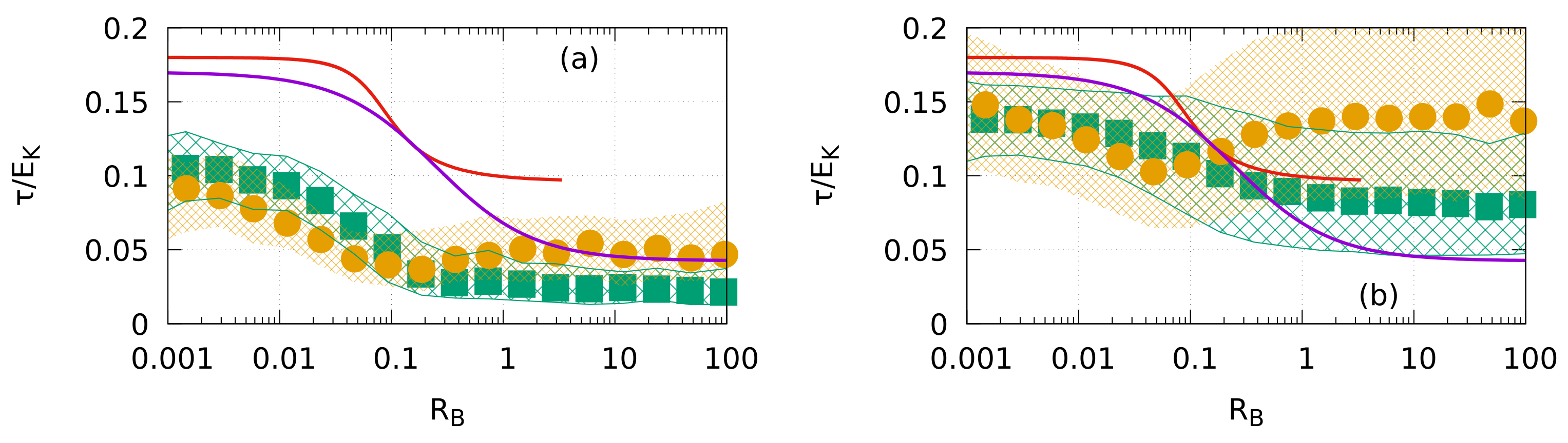
2.4. Remarks about Second-Order Moments

According to MOST, the normalized second-order moments can be expressed as functions of L (see, e.g., [11,19]). For instance, under near-neutral conditions (and under stable conditions, within the so-called z-less limit (see for instance [20])), the ratio between the velocity component variances and the momentum flux read:
u i 2 τ = γ i
with γ i 5.3 , 4 , 1.6 for i = 1 , 2 , 3 , respectively, [11,19].
Under stable conditions, the normalized moments are expected to be dependent on stability, but because of self-correlation, the relations fitted on the data may give ambiguous results. To overcome the problem, Mauritsen and Svensson [21] used the bulk Richardson number as a stability parameter, and observed that τ / E and w θ / [ E θ 2 ] 1 / 2 are both critically dependent on the Richardson number, showing a well-defined change in the Richardson number from 0.1 and 1. This behavior has been treated by Zilitinkevich et al. [6] and reviewed by Li et al. [22] in the frame of models without a critical Richardson number. If instead of taking under exam E / τ the normalized horizontal and vertical variances of the velocity are considered, the behavior may be different, as suggested for instance by Juang et al. [23].

3. Site and Dataset

The Jang Bogo station, managed by the Korea Polar Research Institute (KOPRI), was opened in February 2014 and is located in the coastal region of Terra Nova Bay, Antarctica (74 37 26 S, 164 13 43 E). The station is surrounded by hills up to ∼670 m high from the west to the northeast within a 2 km distance and most of land gently slopes close to the coast. This area is mainly composed of exposed bedrock and glacial moraines. The station is operative all year-round. During summer, with slightly positive temperatures, even for short periods, some of the area of the station grounds is exposed (i.e., free of snow), while all the area is covered with snow and ice during non-summer seasons.
An automated weather station (AWS) was installed when the station was opened, at approximately 150 m east from the main building, acting as a reference for the meteorological conditions at the station. Based on seasonal statistics obtained from single 10 min averages for the years 2016–2019, we found that temperatures are always well below freezing all year-round, except during the austral summer, when the seasonal averages are negative by a few degrees. On the contrary, the winter is very harsh, with average values lower than −20 C. Prevailing winds are from the north/west to the south/west sector during the whole year, while during summer this sector expand towards the south and even the east. Seasonal average speed ranges between 3 and 4 m/s, but the 90th percentile can be higher by as much as 10 m/s. Many other atmospheric observations are routinely carried out at the station, including for radiation (shortwave, longwave, UV), green-house gas and aerosols. A meteorological radiosonde is routinely launched once per day at noon (UTC), while an ozonesonde is routinely launched once per week.
A 9 m tower for meteorological and turbulence measurements was also installed in 2014 upwind from the station, in the west to northeast direction. Turbulence statistics and mean values for three wind components and temperature (corrected for crosswind and humidity effects) were obtained from two sonic anemometers (Campbell scientific model CSAT3), which were mounted facing west at a height of 2 and 9 m of the tower. As declared by the manufacturer, the resolution for the wind components u and v is 1 mm/s (RMS), 0.5 mm/s for w and 0.002 C for temperature (the last at 25 C, might increase the value at very low temperatures). The accuracy is only known for wind speed: <±8.0 cm/s (u, v), <±4.0 cm/s (w). Since air temperature does not fall below −40 C, the sonic anemometers worked year-round. Flow distortion by the tower is not likely significant for a 9 m-high sonic anemometer in any direction but could be significant for a 2 m-high one from the northeast to southeast. Therefore, we analyzed data for wind direction from 180 to 360 .
Raw data at a sampling rate of 20 Hz from both the two sonic anemometers were recorded on a data logger, and then regularly retrieved to a computer in a laboratory. For this work, the data for 2016–2019 were analyzed over time intervals of 30, 10 and 2 min, in order to investigate the different behavior of fluctuations at different frequencies. As a general statement, shorter time intervals tend to filter out low-frequencies phenomena, such as submeso motions. These generally include a rich variety of motions on horizontal scales larger than the turbulence but smaller than a few kilometers. The 30 min results will include a large fraction of the low-frequency fluctuations, although not all of them. For the main part of this work, the two extreme cases (30 and 2 min intervals) were used in order to distinguish which are the quantities affected by submeso motions. A total of 20,329 and 407,003 cases were obtained for the two cases, respectively.

4. Results

4.1. Effect of the Averaging Time Interval

As a preliminary analysis, we discuss in short the effect of the length of the averaging time interval on the statistics we are concerned with.
As introduced above, using different averaging time intervals on a time series is equivalent to applying a box filter, which selects (even approximately) a frequency range in the spectrum ([24], Equation 13.1). Thus, using different intervals corresponds to select different frequency ranges, and we shall use this simple tool to investigate the presence and the effects of the low-frequency (submeso) motions on the turbulence statistics.
In Table 1, the median values for horizontal ( u 2 + v 2 ) and vertical ( w 2 ) velocity variances are reported for different averaging time intervals, for different stability conditions and for the two measuring levels. In passing, note that reading the table by row gives evidence of the effects of averaging time, while reading by column allows to guess the vertical divergence of the variances (see Section 4.2). Similarly, in Table 2, the median values for the vertical fluxes of momentum τ and heat w θ are reported.
We already noticed that the increase in the length of the averaging time interval allows the statistics to include low-frequency motions. Under near-neutral conditions, w 2 is practically unaffected by the length of the interval, i.e., it is mainly affected by the high-frequency (small-scale) eddies, while u 2 + v 2 is reduced by approximately 30 ÷ 40 % (at least for the measurements at 2 m) from 30 min to 2 min averaging times, indicating a contribution by such eddies. Under stable conditions, the reduction is quite evident both for the horizontal and the vertical velocity variances, suggesting that low-frequency motions affect both, to a larger extent for u 2 + v 2 with respect to w 2 , and for 9 m measurements with respect to 2 m.
As regards the fluxes, under near neutral conditions both are practically unaffected by the averaging time interval length at both heights. Under more stable conditions, again at both heights, the interval length affects the momentum flux, and to a smaller extent, the heat flux; as for overall observations, fluxes are less affected than the horizontal variance by the averaging time interval length. As a consequence, the estimate of the Obukhov length is less affected by the choice of the averaging time than the velocity variances, at least for this specific dataset (see Section 4.3).

4.2. Vertical Structure (Divergence) of the Layer

As noted above, an inspection by columns of the Table 1 and Table 2 suggests that the vertical divergence of the second-order moments is a common feature of this surface layer.
A quantitative evaluation of the divergence of a generic quantity x is given by the ratio between the difference of the values of x at the upper and lower levels of the observation and its mean value in the layer between the two levels:
I x = Δ x / x ¯ .
The indexes for the variances of the horizontal and vertical components of the velocity and for the vertical fluxes as a function of the bulk Richardson number and for 30 min and 2 min averages are reported in Figure 1.
From Figure 1a (see also Table 1), the results show that, for 30 min averages, under almost neutral conditions, the vertical divergence is negligible on the median, although a 10% increment can be observed for w 2 , while under stable conditions, there is an increase in the horizontal velocity variance of approximately 20% in height and by more than 100% for the vertical velocity variance.
The different behavior of the index I for horizontal and vertical velocity variances under stable conditions is related to the buoyancy damping of the vertical motions, while horizontal motions are less affected, as can be seen [25].
From Figure 1b (see also Table 2), it is interesting to note that the vertical momentum flux τ slightly decreases in height under near neutral conditions, and in median (but the distribution is quite large) increases of more that 100% in stable cases. A different behavior is found for the heat flux, which shows an increase in height under near neutral conditions (though it is quite small in these cases) while it is almost constant on average under stable conditions.
With regard to the 2 min averages, as can be seen in Figure 1c,d, the results show that the general behavior is similar to that of the 30 min averages, but with values of divergence that are smaller on average and at the same time more dispersed, so much so that in the case of horizontal velocity, they pass from purely positive to a distribution with almost half the negative values. In other words, the vertical divergence is mainly associated with the low-frequency motions.
It may be worth noticing that Högström et al. [8] discussed the increase in vertical velocity variance in the surface layer as related to the blocking due to the surface.

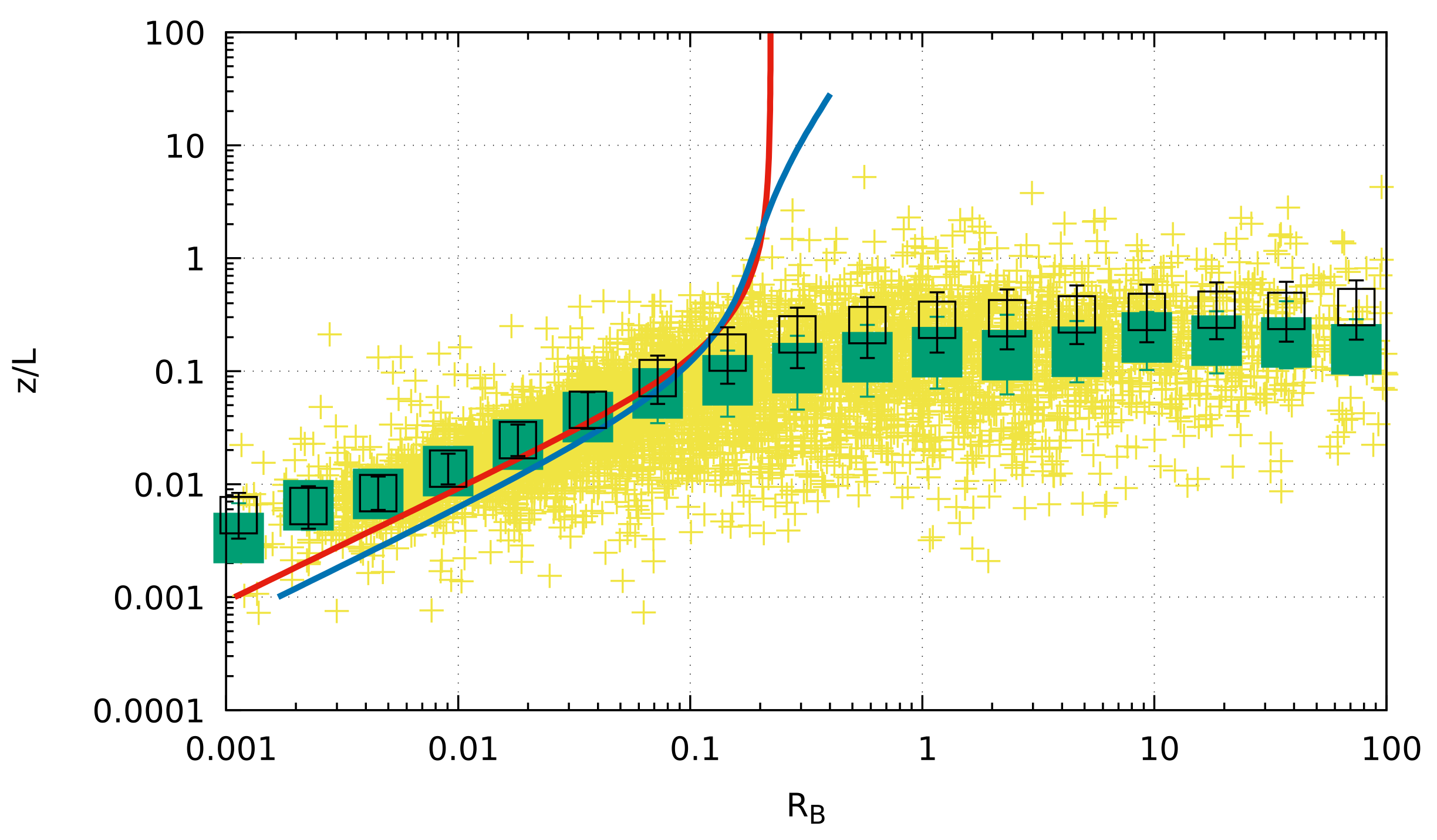
4.3. The Obukhov Length and the Richardson Number

The inverse of the Obukhov length, computed using the mean values of the fluxes in the 2 ÷ 9 m layer, is reported as a function of the bulk Richardson number in Figure 2. In order to present a non-dimensional variable, in the figure, the quantity z / L with z = 2.5 m is plotted; the height is quite arbitrarily chosen in the layer of interest and it must be noted that any choice does not affect the physical meaning of the observations. It results that R B steadily increases while z / L diverges for R B 0.2 . The empirical dependence of z / L from R B is well described by the relation derived from the mean profiles for R B 0.1 ; the log-linear profiles (by integration of Equations (3) and (4)) predict a critical value of approximately 0.21 , while the profiles suggested by Gryanik et al. [17] exhibit an increase for R B at 1 < z / L < 10 —in any case, their validity is limited to z / L < 100 .
Moreover, the different time averaging intervals almost do not affect the distribution of data, consistently with the observations that the fluxes show a minor influence of the length of the averaging interval.
This result supports and justifies the choice of Richardson number as a measure of stability: in fact, many observations would collapse in a small interval of z / L around 0.25 , while being well distributed in the range R B > 0.2 .

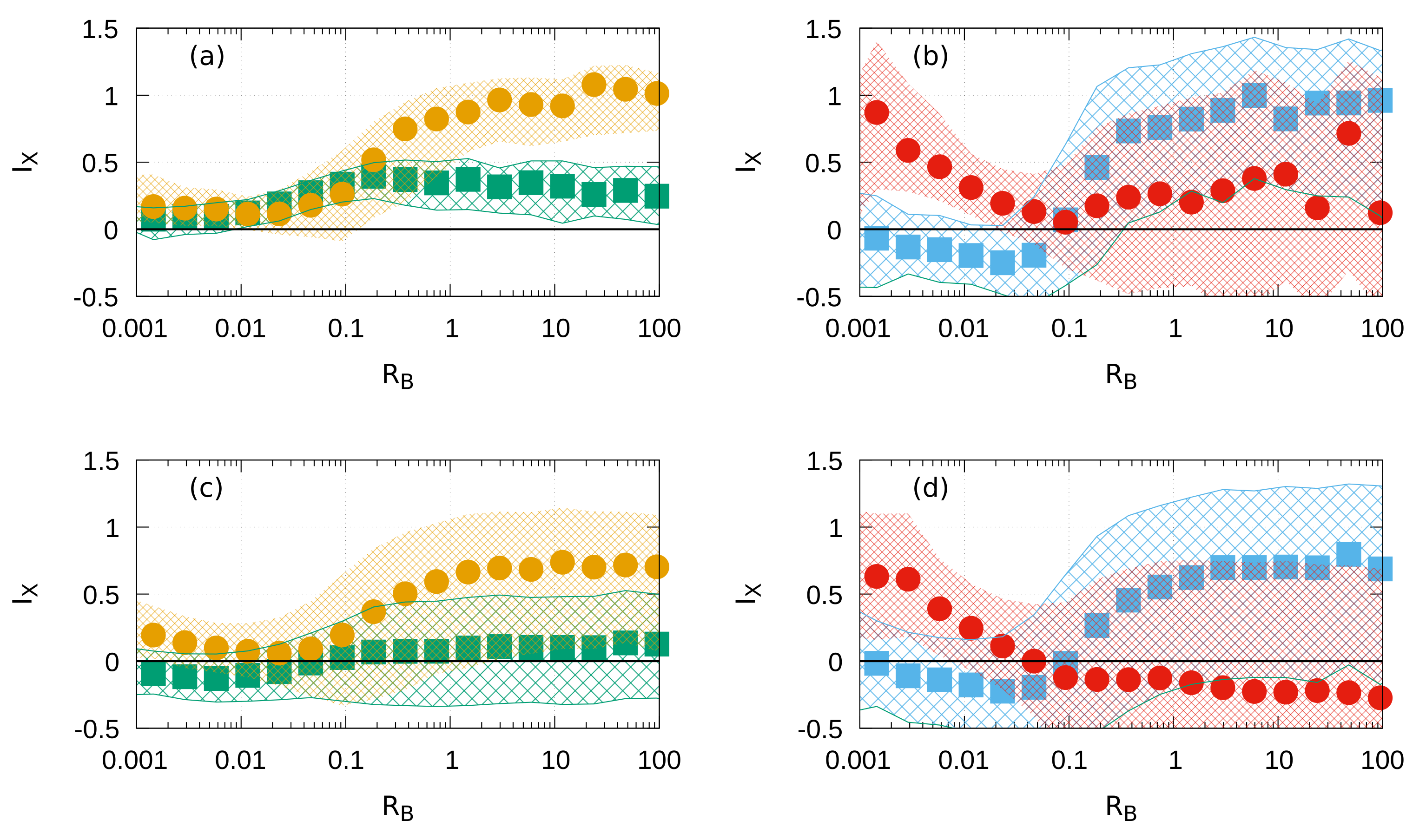
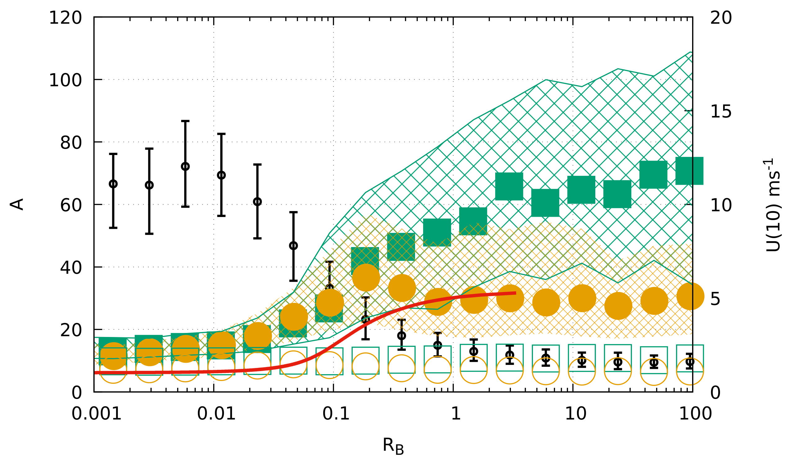
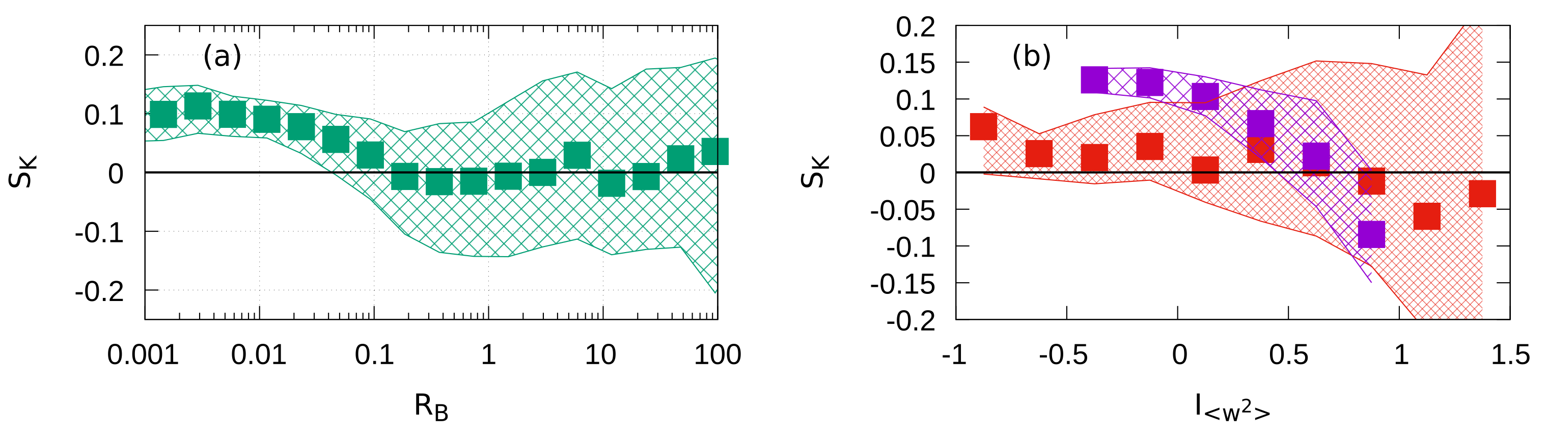
4.4. Turbulence Characterization

In this subsection, we analyze the behavior of some characteristic quantities as a function of the bulk Richardson number.
The anisotropy ratio A:
A = u 2 + v 2 w 2
is a measure of the share of the TKE between the horizontal and vertical components of velocity and is characterized by an almost universal value A 5 ÷ 6 for the shear produced by turbulence (i.e., under near-neutral or weakly stable conditions), while it presents a large variability under strong stability conditions A 15 ÷ 30 (as can be seen, for instance, in Zilitinkevich et al. ([6], Figure 6), Tampieri ([11], Figure 3.29)).
In the frame of this analysis, we limited ourselves to the examination of second-order moments, and did not use the spectra. Thus, the anisotropy ratio has a two-fold meaning: it increases its value from neutral to stable conditions, and also increases its value in the presence of submeso motions (which typically affect the horizontal more than the vertical velocity variances). In the following discussion, we shall outline how to separate (at least statistically) the two aspects.
The anisotropy ratio A is shown in Figure 3 as a function of R B .
Under near neutral conditions (say, R B < 0.02 ), A is quite similar at the two levels, and its values for the 2 min averages are only slightly smaller than the ones for the 30 min averages. Broadly, the data are quite in agreement with the theoretical value from [6], with modified coefficients: Zilitinkevich and coworkers (private communication) did re-evaluate the coefficients of the 2013 model using further atmospheric observations and LES simulations, so the coefficients we use are slightly different from the published ones.
Under stable conditions (e.g., R B > 0.5 ), the ratio A for 30 min averages increases, and its variability also increases; the increase and the spread around the median are much more evident at the lowest level. This difference between the two levels occurs because w 2 increases with height while u 2 + v 2 much less, as discussed before. The A ratios for 2 min averaged data are quite similar to the ones of the near neutral case, thus practically independent on stability.
The theoretical values predicted by Zilitinkevich et al. [6] show fairly good agreement for near neutral conditions, and at larger R B only for the observations at z = 9 m averaged over 30 min. A major change related to the increase in stability occurs at z = 2 m for the 30 min averaged data, while the 2 min averaged data appear to be almost independent from stability.
In Figure 3, the wind velocity binned for R B intervals is also reported (black symbols). The wind velocity reaches the highest values under near neutral conditions and drops to very small values with increasing stability, thus supporting the empirical evidence of minor effects of submeso motions (which are a reason for the increase in the ratio A) under strong wind conditions. In fact, submeso motions are mainly detected under low-wind conditions (see, for instance [26,27,28]).
The ratio τ / E K is shown in Figure 4 as a function of R B and compared with the Mauritsen and Svensson [21] empirical relation and the Zilitinkevich et al. [6] theoretical curve.
This ratio shows a relevant decrease with stability, in qualitative agreement with the literature, for both 30 min data and 2 min data. Note that the overall values of the ratio are larger for 2 min than for 30 min averages, and that our 30 min averages are smaller than those presented by Mauritsen and Svensson [21] which refer, for all but one dataset, to averaging times of 5 min or 10 min, supporting the view that TKE (to be more precise, the horizontal velocity variance) is more influenced than fluxes by the submeso motions.
Similar considerations hold for the normalized vertical heat flux H = w θ / [ E K θ 2 ] 1 / 2 , shown in Figure 5. It is worth noticing that the normalized heat flux has a minimum for 0.01 < R B < 0.1 , which is well documented by the observations [11,21] but not represented in the empirical curve by Mauritsen and Svensson [21] nor theoretically predicted by Zilitinkevich et al. [6].
The skewness of the vertical velocity S K = w 3 / w 2 3 / 2 , averaged over the 2 ÷ 9 m layer, for 30 min averaging time, is reported in Figure 6. It is positive under near neutral conditions, while under stable conditions, the median value approaches zero with a wide fluctuation range.
It is worth noticing that, under near-neutral conditions, the skewness is on median positive, basically due to the surface blocking effect. Consistently, the large variability (with zero median) under stable conditions corresponds to the reduction in the vertical scale length. Note also (right panel) that the skewness in near-neutral cases decreases with the vertical divergence of w 2 . From a flux–gradient perspective, skewness is expected to be zero for I w = 0 . Actually, w 3 / w 2 3 / 2 0 at I w 0.6 , again highlighting the importance of surface blocking. In the stable case, the skewness is in median near zero, consistent with the literature—as can be seen in Barberis [29], from the data of Higgins et al. [30]. It is worth noticing that the spread (25–75% percentiles) increases steadily with the index I w 2 , consistent with the general consideration that the decoupling between the layers (and thus the vertical velocity distribution may be quite different from case to case) is the dominant factor characterizing such a surface layer.

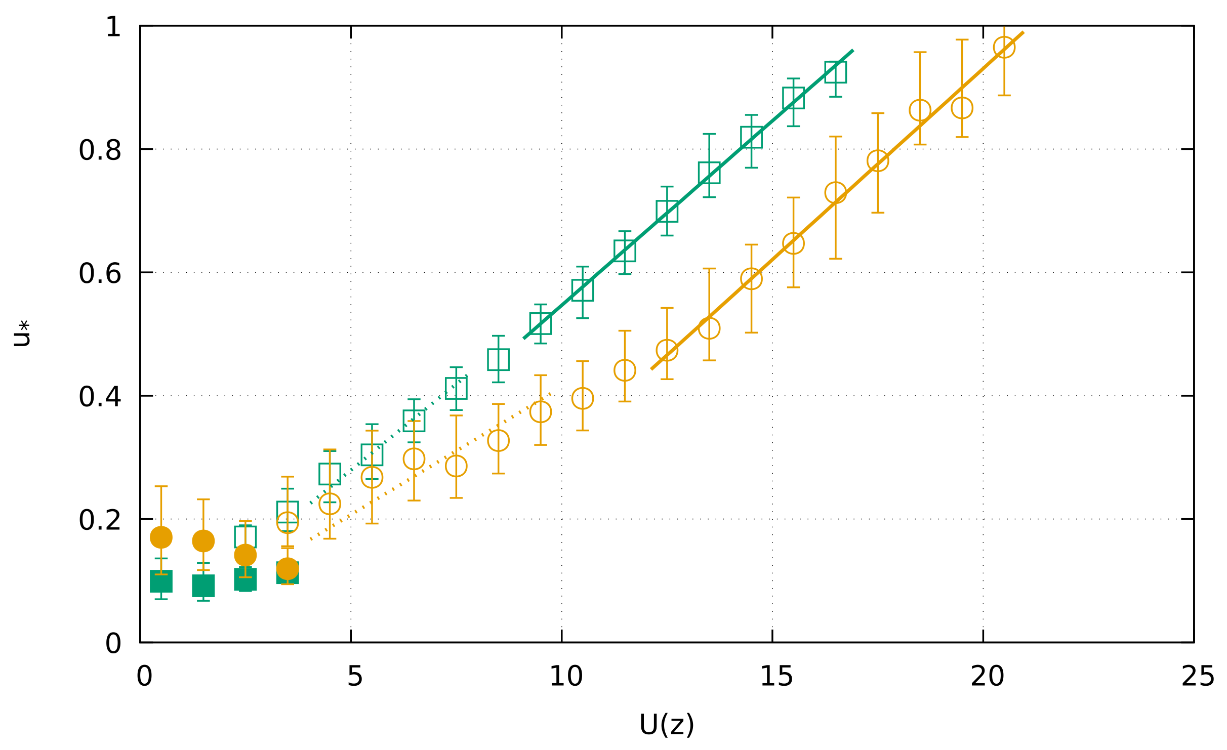
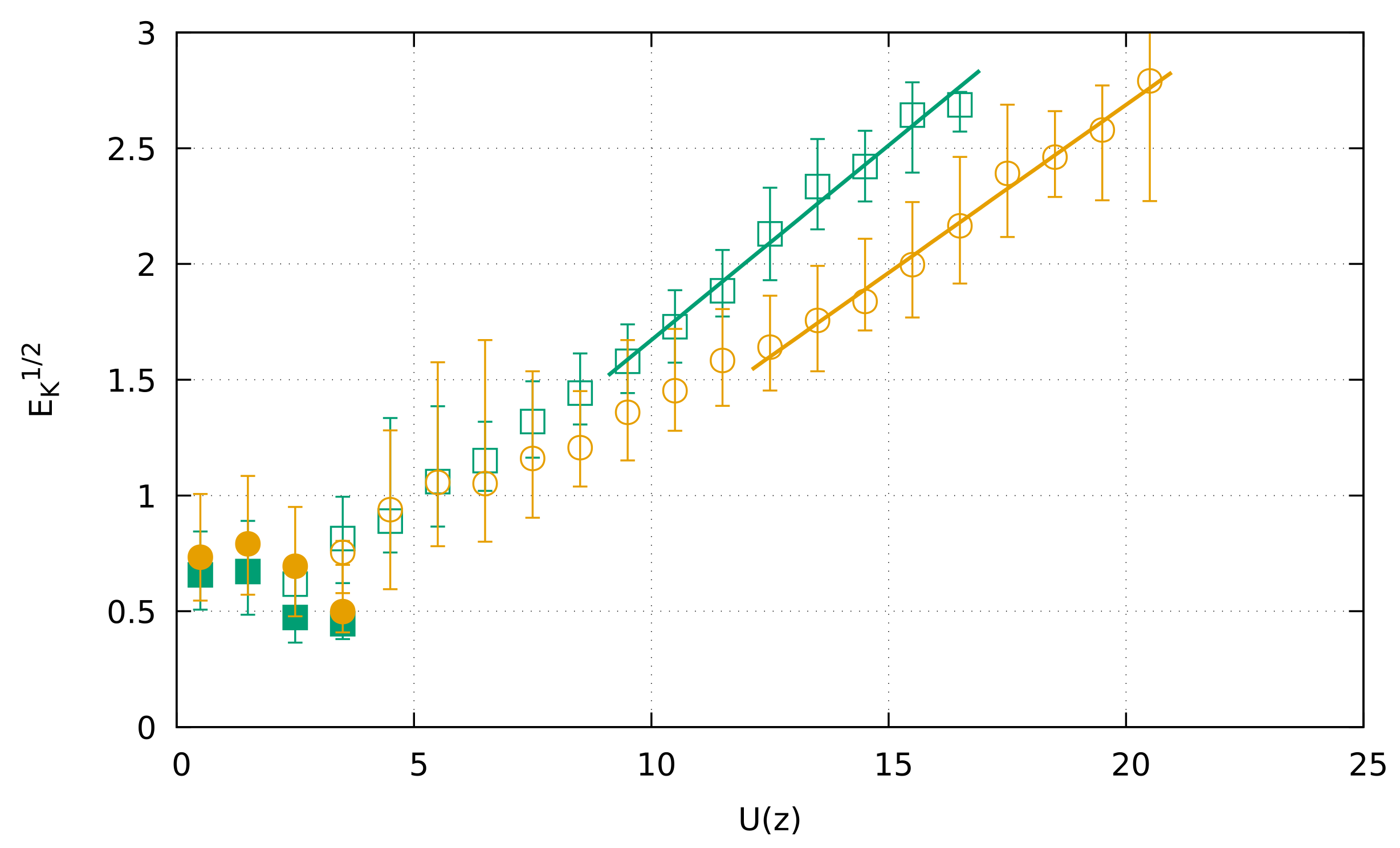
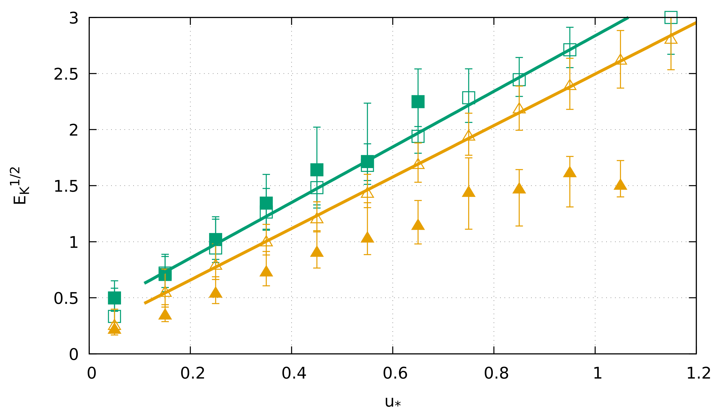
4.5. The Behavior of the Turbulence Velocities

In this subsection, the behavior of E K and of u * , also called ‘turbulence velocities’, is analyzed as function of the wind velocity U, following the line of Sun et al. [3].
The plot of u * ( z ) vs. U ( z ) is reported in Figure 7 and has the general features of the HOST paradigm:
  • For near-neutral conditions:
MOST, i.e., Equation (9), is valid from approximately 4 m/s to approximately 8 m/s for z = 2 m, to approximately 10 m/s for z = 9 m; these threshold velocities are quite a bit larger than those observed in the CASES-99 experiment ([5], Figure 6); the roughness (derived from the fit of the log profile) is different for the two levels ( z 0 2.5 × 10 3 at 2 m, z 0 10 3 at 9 m) suggesting the existence of an internal boundary layer;
The slope beyond the threshold velocity is 0.06 (smaller than the 0.1 value shown by Sun et al. ([5], Figure 6));
  • For all the stability conditions, and for both the averaging times, τ 0 as U 0 .
All these observations are the same for both 30 min and 2 min averaging intervals (not shown), quite consistent with the observation made before about the minor influence of the averaging time on the vertical momentum flux.
The relationship between E K 1 / 2 and U ( z ) is exploited in Figure 8, to be compared with Sun et al. ([3], Figure 1).
Under near neutral conditions, beyond the threshold velocity, the slope is approximately 0.17 at z = 2 m and 0.15 at z = 9 m for a 30 min averaging time (slightly less for 2 min averaging time at z = 9 m), smaller than the value resulting from Sun et al. [3]. Under stable conditions, E 1 / 2 does not increase with the wind velocity for a 30 min averaging time. In general, the observations also support the existence of some level of TKE for the wind velocity decreasing to zero, associated with the low-frequency motions and not to the shear.
These results confirm the general HOST frame and at the same time stress the fact that the numerical values of the threshold velocity and of the slope are (at least) site dependent.
A final remark about turbulence velocities is suggested by the application of Equation (8), as reported in Figure 9.
We obtain the result that the data for near-neutral conditions approximately follow Equation (8), neglecting the values for small friction velocity, say for u * < 0.1 , with a slope giving α B 0.22 for the 2 min averaging time, in quite good agreement with the value suggested by Basu et al. [18]. For stable conditions, the TKE of 30 min averaged data is larger than that of the near-neutral ones, suggesting that part of the TKE is supplied by sources different from the shear production, while the 2 min averaged data show less TKE than the near-neutral ones, because the influence of the low-frequency motions is small or negligible.

5. Conclusions

The statistical analysis of the 5-year dataset of turbulence measurements at Jang Bogo Station confirmed some literature results and evidenced some important new features.
The effects of the averaging time were discussed—it was shown to be more relevant to the variances of the velocity components than on the vertical fluxes. This leads to recognize that the Obukhov length (as well as the Richardson number) cannot be used as the only parameter to model for instance the dependence of the TKE averaged for 30 min on z / L , because TKE may be influenced by low-frequency motions that only have a marginal effect on L and do not directly depend on stability, although they occur more frequently under stable conditions.
All the normalized second-order moments investigated herein exhibit a well-defined change in the range 0.1 < R B < 1 , thus confirming literature results, although the absolute values can be site-dependent, and also time-averaging interval length dependent.
The vertical divergence of the second-order moments is shown to be a common feature of this boundary layer. In particular, the divergence of the vertical velocity variance is put into relation with the vertical velocity skewness, evidencing that in a relevant range of the parameter I w , the flux–gradient relation is not satisfied. More generally, this observation is also supported by the behavior of the turbulent velocities for the mean velocity approaching zero.

Author Contributions

Conceptualization, A.P.V. and F.T.; Data curation, M.M.; Formal analysis, F.T.; Funding acquisition, M.M. and T.C.; Investigation, M.M., A.P.V., T.C. and F.T.; Methodology, F.T.; Project administration, M.M. and T.C.; Resources, M.M.; Software, M.M.; Supervision, M.M., T.C. and F.T.; Writing—original draft, F.T.; Writing—review & editing, M.M., A.P.V. and T.C. All authors have read and agreed to the published version of the manuscript.

Funding

This research was funded by the Italian National Program of Research in Antarctica (PNRA), project n. PNRA16_00031, Surface-Atmosphere Mass and Energy Exchanges at a Coastal Antarctic Site (SAMEECA).

Data Availability Statement

Data are available through direct contact with the authors.

Acknowledgments

The authors acknowledge KOPRI and the technical staff of Jang Bogo Station for their support in continuously running the instrumentation.

Conflicts of Interest

The authors declare no conflict of interest.

References

  1. Nieuwstadt, F.T.M. The turbulent structure of the stable, nocturnal boundary layer. J. Atmos. Sci. 1984, 41, 2202–2216. [Google Scholar] [CrossRef]
  2. Grachev, A.A.; Andreas, E.L.; Fairall, C.W.; Guest, P.S.; Persson, P.O.G. The Critical Richardson Number and Limits of Applicability of Local Similarity Theory in the Stable Boundary Layer. Bound. Layer Meteorol. 2013, 147, 51–82. [Google Scholar] [CrossRef] [Green Version]
  3. Sun, J.; Mahrt, L.; Banta, R.M.; Pichugina, Y.L. Turbulence regimes and turbulence intermittency in the stable boundary layer during CASES-99. J. Atmos. Sci. 2012, 69, 338–351. [Google Scholar] [CrossRef] [Green Version]
  4. Sun, J.; Lenschow, D.H.; LeMone, M.A.; Mahrt, L. The role of large-coherent-eddy transport in the atmospheric surface layer based on CASES-99 observations. Bound. Layer Meteorol. 2016, 160, 83–111. [Google Scholar] [CrossRef]
  5. Sun, J.; Takle, E.S.; Acevedo, O.C. Understanding Physical Processes Represented by the Monin–Obukhov Bulk Formula for Momentum Transfer. Bound. Layer Meteorol. 2020, 177, 69–95. [Google Scholar] [CrossRef]
  6. Zilitinkevich, S.S.; Elperin, T.; Kleeorin, N.; Rogachevskii, I.; Esau, I.N. A Hierarchy of Energy- and Flux-Budget (EFB) Turbulence Closure Models for Stably-Stratified Geophysical Flows. Bound. Layer Meteorol. 2013, 146, 341–373. [Google Scholar] [CrossRef] [Green Version]
  7. Cheng, Y.; Canuto, V.; Howard, A.; Ackerman, A.S.; Kelley, M.; Fridlind, A.M.; Schmidt, G.A.; Yao, M.S.; Del Genio, A.; Elsaesser, G.S. A Second-Order Closure Turbulence Model: New Heat Flux Equations and No Critical Richardson Number. J. Atmos. Sci. 2020, 77, 2743–2759. [Google Scholar] [CrossRef]
  8. Högström, U.; Hunt, J.C.R.; Smedman, A.S. Theory and measurements for turbulence spectra and variances in the atmospheric neutral surface layer. Bound. Layer Meteorol. 2002, 103, 101–124. [Google Scholar] [CrossRef]
  9. Mahrt, L.; Vickers, D. Contrasting vertical structures of nocturnal boundary layers. Bound. Layer Meteorol. 2002, 105, 351–363. [Google Scholar] [CrossRef]
  10. Mahrt, L.; Thomas, C.; Grachev, A.A.; Persson, P.O.G. Near-Surface Vertical Flux Divergence in the Stable Boundary Layer. Bound. Layer Meteorol. 2018, 169, 373–393. [Google Scholar] [CrossRef]
  11. Tampieri, F. Turbulence and Dispersion in the Planetary Boundary Layer; Springer International: Basel, Switzerland, 2017. [Google Scholar]
  12. Monin, A.; Obukhov, A. Basic laws of turbulent mixing in the surface layer of the atmosphere. Contrib. Geophys. Inst. Acad. Sci. USSR 1954, 151, e187. [Google Scholar]
  13. Högström, U. Non-dimensional wind and temperature profiles in the atmospheric surface layer: A re-evaluation. Bound. Layer Meteorol. 1988, 42, 55–78. [Google Scholar] [CrossRef]
  14. Grachev, A.A.; Fairall, C.W.; Persson, P.O.G.; Andreas, E.L.; Guest, P.S. Stable Boundary-Layer Scaling Regimes: The Sheba Data. Bound. Layer Meteorol. 2005, 116, 201–235. [Google Scholar] [CrossRef]
  15. van Ulden, A.P.; Holtslag, A.A.M. Estimation of atmospheric boundary layer parameters for diffusion applications. J. Clim. Appl. Meteorol. 1985, 24, 1196–1207. [Google Scholar] [CrossRef] [Green Version]
  16. Yagüe, C.; Viana, S.; Maqueda, G.; Redondo, J.M. Influence of stability on the flux-profile relationships for wind speed, Φm, and temperature, Φh, for the stable atmospheric boundary layer. Nonlinear Proc. Geophys. 2006, 13, 185–203. [Google Scholar] [CrossRef] [Green Version]
  17. Gryanik, V.M.; Luepkes, C.; Grachev, A.A.; Sidorenko, D. New modified and extended stability functions for the stable boundary layer based on SHEBA and parametrizations of bulk transfer coefficients for climate models. J. Atmos. Sci. 2020, 77, 2687–2716. [Google Scholar] [CrossRef]
  18. Basu, S.; He, P.; DeMarco, A.W. Parametrizing the Energy Dissipation Rate in Stably Stratified Flows. Bound. Layer Meteorol. 2021, 178, 167–184. [Google Scholar] [CrossRef]
  19. Grachev, A.A.; Leo, L.S.; Di Sabatino, S.; Fernando, H.J.S.; Pardyjak, E.R.; Fairall, C.W. Structure of Turbulence in Katabatic Flows Below and Above the Wind-Speed Maximum. Bound. Layer Meteorol. 2016, 159, 469–494. [Google Scholar] [CrossRef] [Green Version]
  20. Wyngaard, J.C.; Coté, O.R. Cospectral similarity in the atmospheric surface layer. Q. J. R. Meteorol. Soc. 1972, 98, 590–603. [Google Scholar] [CrossRef]
  21. Mauritsen, T.; Svensson, G. Observations of Stably Stratified Shear-Driven Atmospheric Turbulence at Low and High Richardson Numbers. J. Atmos. Sci. 2007, 64, 645–655. [Google Scholar] [CrossRef]
  22. Li, D.; Katul, G.G.; Zilitinkevich, S.S. Closure schemes for stably stratified atmospheric flows without turbulence cutoff. J. Atmos. Sci. 2016, 73, 4817–4832. [Google Scholar] [CrossRef] [Green Version]
  23. Juang, J.Y.; Katul, G.G.; Siqueira, M.B.; Stoy, P.C.; McCarthy, H.R. Investigating a hierarchy of Eulerian closure models for scalar transfer inside forested canopies. Bound. Layer Meteorol. 2008, 128, 1–32. [Google Scholar] [CrossRef] [Green Version]
  24. Pope, S. Turbulent Flows; Cambridge University Press: Cambridge, UK, 2000. [Google Scholar]
  25. Lindborg, E. The energy cascade in a strongly stratified fluid. J. Fluid Mech. 2006, 550, 207–242. [Google Scholar] [CrossRef]
  26. Anfossi, D.; Oettl, D.; Degrazia, G.; Ferrero, E.; Goulart, A. An analysis of sonic anemometer observations in low wind speed conditions. Bound. Layer Meteorol. 2005, 114, 179–203. [Google Scholar] [CrossRef]
  27. Mortarini, L.; Cava, D.; Giostra, U.; Costa, F.D.; Degrazia, G.; Anfossi, D.; Acevedo, O. Horizontal meandering as a distinctive feature of the Stable Boundary Layer. J. Atmos. Sci. 2019, 76, 3029–3046. [Google Scholar] [CrossRef]
  28. Schiavon, M.; Tampieri, F.; Bosveld, F.; Mazzola, M.; Castelli, S.T.; Viola, A.; Yagüe, C. The Share of the Mean Turbulent Kinetic Energy in the Near-Neutral Surface Layer for High and Low Wind Speeds. Bound. Layer Meteorol. 2019, 172, 81–106. [Google Scholar] [CrossRef]
  29. Barberis, E. Analisi Statistiche Nello Strato Limite Turbolento. Ph.D. Thesis, Dipartimento di Fisica Teorica, Università degli Studi di Torino, Torino, Italy, 2007. [Google Scholar]
  30. Higgins, C.W.; Meneveau, C.; Parlange, M. The effect of filter dimension on the subgrid-scale stress, heat flux, and tensor alignements in the atmospheric surface layer. J. Atmos. Ocean Technol. 2007, 24, 360–375. [Google Scholar] [CrossRef]
Figure 1. Median values (symbols) and the range of 25–75% percentiles (filled areas) as a function of R B for: I u 2 + v 2 (green squares) and I w 2 (brown dots) (a,c); I τ (blue squares) and I w θ (red dots) (b,d). (a,b) are for 30 min averaging time; (c,d) are for 2 min averaging time.
Atmosphere 12 01095 g001
Figure 2. z / L computed using the turbulent fluxes averaged in the 2 ÷ 9 m layer vs. R B . Yellow: all the 30 min averaged data; green squares with error bars: binned 30 min averaged data, medians and 25–75% percentiles. Black open squares: binned 2 min averaged data. The red line shows the relationship arising from the log-linear non-dimensional profiles, from the integration of Equations (3) and (4). The blue line refers to the profiles by Gryanik et al. ([17], Equations 34 and 35).
Atmosphere 12 01095 g002
Figure 3. A as a function of R B . Squares and the shaded green area are the median and the range 25–75% percentiles for observations at z = 2 m; dots and brown area the same for z = 9 m; both averaged over 30 min. The open symbols correspond to the medians for data averaged over 2 min. Small black circles with error bars indicate the wind velocity measured at z = 10 m on the neighboring mast. The red line corresponds to the theoretical behavior from [6].
Atmosphere 12 01095 g003
Figure 4. τ / E K as function of R B : (a) 30 min averages; and (b) 2 min averages. Symbols and colors are the same as in Figure 1a. The red line corresponds to the theoretical behavior from [6], with modified coefficients, the violet one to Mauritsen and Svensson [21].
Atmosphere 12 01095 g004
Figure 5. Normalized vertical heat flux H = w θ / [ E K θ 2 ] 1 / 2 as function of R B : (a) 30 min averages; and (b) 2 min averages. Symbols, colors and lines are the same as in Figure 1a and Figure 4.
Atmosphere 12 01095 g005
Figure 6. (a) Vertical velocity skewness S K = w 3 / w 2 3 / 2 (30 min averaged) vs. R B . Symbols and colors are the same as in Figure 1a; (b) S K vs. I w 2 for near-neutral cases (blue) and stable cases (red).
Atmosphere 12 01095 g006
Figure 7. u * ( z ) vs. U ( z ) , for 30 min averaging intervals. Open symbols: near neutral conditions; closed symbols: stable conditions; green: z = 2 m, brown: z = 9 m. Lines from the fits: dotted lines, MOST similarity below the threshold velocity; continuous lines: HOST large wind behavior, beyond the threshold velocity.
Atmosphere 12 01095 g007
Figure 8. E K vs. U ( z ) , for 30 min averaging intervals. Symbols and colors as in Figure 7.
Atmosphere 12 01095 g008
Figure 9. E K vs. u * , averaged over the layer 2 ÷ 9 m. Open symbols: near neutral conditions, closed symbols: stable conditions; squares: 30 min averaging time, triangles: 2 min averaging time. Lines: linear fit in the range u * > 0.1 .
Atmosphere 12 01095 g009
Table 1. Median values for horizontal and vertical velocity variances (in m 2 s 2 ) measured at the two heights, for different stability conditions and different time intervals.
30 min 10 min2 min
0.001 < R B < 0.01
u 2 + v 2 (2 m)4.23.83.0
u 2 + v 2 (9 m)4.53.92.6
w 2 (2 m)0.280.290.29
w 2 (9 m)0.330.330.33
1 < R B < 10
u 2 + v 2 (2 m)0.800.400.13
u 2 + v 2 (9 m)1.040.480.14
w 2 (2 m)0.0150.0140.012
w 2 (9 m)0.0350.0290.019
Table 2. As in Table 1, but for the vertical fluxes of momentum τ (in m 2 s 2 ) and of heat w θ (in K m s 1 ).
30 min 10 min 2 min
0.001 < R B < 0.01
τ (2 m)0.220.220.22
τ (9 m)0.190.190.18
w θ (2 m)−0.016−0.016−0.018
w θ (9 m)−0.028−0.028−0.029
1 < R B < 10
τ (2 m)0.0090.0080.006
τ (9 m)0.0240.0180.011
w θ (2 m)−0.008−0.008−0.007
w θ (9 m)−0.010−0.009−0.006
Publisher’s Note: MDPI stays neutral with regard to jurisdictional claims in published maps and institutional affiliations.

