An Atmospheric Visibility Grading Method Based on Ensemble Learning and Stochastic Weight Average

Abstract

In order to adequately characterize the visual characteristics of atmospheric visibility and overcome the disadvantages of the traditional atmospheric visibility measurement method with significant dependence on preset reference objects, high cost, and complicated steps, this paper proposed an ensemble learning method for atmospheric visibility grading based on deep neural network and stochastic weight averaging. An experiment was conducted using the scene of an expressway, and three visibility levels were set, i.e., Level 1, Level 2, and Level 3. Firstly, the EfficientNet was transferred to extract the abstract features of the images. Then, training and grading were performed on the feature sets through the SoftMax regression model. Subsequently, the feature sets were ensembled using the method of stochastic weight averaging to obtain the atmospheric visibility grading model. The obtained datasets were input into the grading model and tested. The grading model classified the results into three categories, with the grading accuracy being 95.00%, 89.45%, and 90.91%, respectively, and the average accuracy of 91.79%. The results obtained by the proposed method were compared with those obtained by the existing methods, and the proposed method showed better performance than those of other methods. This method can be used to classify the atmospheric visibility of traffic and reduce the incidence of traffic accidents caused by atmospheric visibility.

1. Introduction

Atmospheric visibility is a critical item in road meteorological observation, which has an essential impact on traffic safety and human health. In poor weather or haze conditions, the visibility will be significantly reduced, affecting the driver’s judgment, even causing traffic accidents and threatening people’s lives. On the other hand, atmospheric visibility can also reflect the air quality, which is very important for humans, as poor air quality damages human health. Therefore, the grading of atmospheric visibility is of considerable significance to traffic safety and human health.

In meteorology, atmospheric visibility is an indicator that reflects the transparency of the atmosphere [1]. It is generally defined as the maximum ground horizontal distance that a person with normal vision can see the outline of a target clearly under the weather conditions at that time. Traditional visibility measurement methods include the visual inspection method, instrumental measurement method, and image-based grading method. The visual inspection method estimates the atmospheric visibility of a scene through manual observation, and its accuracy is affected by the subjective factors of the observer. The instrumental measurement method uses optical instruments, such as scatterometers or transmissometers [2]. This method has the disadvantages of difficulty in instrument installation, poor operability, high requirement for installation accuracy, and low grading efficiency, which is not conducive to grading atmospheric visibility.

Cameras have been widely used in transportation and security fields in recent years due to the wide vision coverage and rich information contained in images [3,4]. At the same time, the method of analyzing atmospheric visibility using digital images has also made significant progress. Generally, atmospheric visibility is calculated based on the image’s feature value, interest pane, optical contrast of the scene, or their combination, corrected by the histogram or other grading modules. Chen et al. [5] designed a visibility measurement system based on automatic image detection. Using the transmittance calculation formula of the dark channel prior algorithm, the target area where the point with the maximum I^C (color channel) was located in the dark channel was taken as the final target area for visibility measurement. The atmospheric refractive index was used to calculate the atmospheric extinction system and to obtain atmospheric visibility further. The proposed model was highly operable and provided a reference for investigating the traffic accidents caused by agglomerate fog. Tang et al. [6] revealed that learning could adequately reflect the visual features of visibility, and it could be used to solve the problem of the difficulty in constructing large-scale training datasets. They applied deep convolutional neural networks to visibility detection, which solved the problem of constructing large-scale datasets and was beneficial to data ensembling. Bosse et al. [7] proposed an image quality evaluation method based on deep neural networks, which was data-driven and did not rely on prior knowledge of human operations or other human visual systems or image statistics. The cross-database evaluation showed its robust generalization ability in different databases. You et al. [8] proposed a deep learning method that estimated atmospheric visibility directly from outdoor images without relying on weather images or expensive instruments. The method used a large number of images from the Internet to learn vibrant scenes and adapt to visibility changes. The model could be used to predict absolute visibility in limited scenarios but with a higher level of intelligence and fewer requirements for instruments. Nathan et al. [9] used image processing and pattern detection techniques to estimate the atmospheric visibility in image datasets. Zheng et al. [10] of our research team proposed an atmospheric visibility grading algorithm based on vision technology and binary tree support vector machines, which provided an effective solution for grading atmospheric visibility.

The above content shows that deep learning has made a significant breakthrough in the field of machine vision. Deep learning can extract more characteristic image features, and deep neural networks require massive data for training. However, large-scale samples with labeled visibility are often difficult to be constructed. On the one hand, visibility labeling is susceptible to the subjective factors of observers, leading to low labeling accuracy. On the other hand, visibility is easily affected by weather, and bad weather is not typical, so the number of samples with low visibility is small.

The visibility detection of traditional open areas is predicted by regular weather forecasts, but the weather forecast is an inspection of a larger area. Usually, the visibility inspection is not accurate for every traffic road, so it is important for vehicles on the road. The reference value is limited. First of all, it is not easy to calculate the visibility value accurately and strictly. Even professional visibility measuring instruments will have measurement errors, which are often more than 10%. Although image-based measurement is theoretically feasible, it will be limited by the application environment and difficult to promote in practical applications. Secondly, the meaning of the definition of visibility itself is more reflected in the human senses, and people generally can only get the qualitative perception of visibility as “good”, “bad” or “ordinary”, and the specific value of it is not so caring. It is for these considerations that in subsequent articles, we are defining three levels of visibility instead of calculating specific values.

This paper proposed a method based on EfficientNet [11] and ensemble learning to detect atmospheric visibility levels. In this paper, three atmospheric visibility levels were set for specific traffic road scenes. EfficientNet was trained first, and then the trained neural network was ensembled by stochastic weight averaging (SWA) [12] to obtain a visibility grading model.

2. Materials and Methods

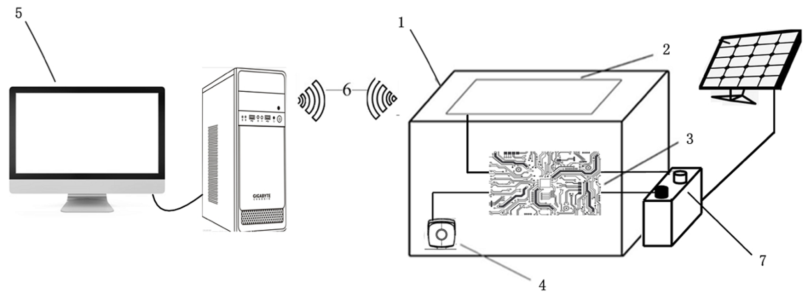
2.1. Materials

In order to analyze the level of atmospheric visibility, an image acquisition device was set up by a Hikvision high-definition camera with a resolution of 5 million pixels and a focal length of 12 mm. The image acquisition device, energy device, and computer constituted the image acquisition system. The experimental device is shown in Figure 1, and the experimental site is on the top floor of the Boyuan Building on the Pukou Campus of Nanjing Agricultural University, China. The device model of the image acquisition device is shown in

Table 1. Device model of the image acquisition device.

Software and Hardware	Model/Version
OS	Windows 10
Camera	Hikvision
Software	Python 3.7
CPU	i5-8500
GPU graphics card	Nvidia RTX 2080
Control host	DSP-DM642

. The images were collected from 5:00 to 18:00 every day from November to December 2019. The collected images were used to establish an atmospheric visibility image dataset. For ensuring the accuracy of visibility grading, the visibility level of each image was determined according to the air pollution index (API) value provided by the Ministry of Ecology and Environment of China (http://106.37.208.233:20035/, accessed on 6 March 2020). Some samples of the acquired images are shown in Figure 2. The image dataset contains a total of 2500 training sets and 500 validation sets.

2.2. Visibility Level

At present, there is no uniform standard for visibility classification. The visibility classification in this paper is mainly based on the air pollution index provided by the China Meteorological Administration, which is divided into three levels. This article is aimed at specific scenes of traffic roads. By detecting the level of visibility, it is recommended that the driver’s safe driving behavior under this visibility is in order to achieve the goal of reducing traffic accidents. In such specific scenarios, the exact value of visibility is not needed; only qualitative perception is needed [13].

The visibility labeling process in this article is: first through the real-time collection of images, and then according to the time the image was taken and the air pollution index (API) released by the China Meteorological Administration at that time and the place (data source: http://106.37.208.233:20035/, accessed on 6 March 2020), correspondingly, so as to classify and mark the visibility of the image. The flow chart of atmospheric visibility classification is shown in Figure 3.

From

Table 2. The definition of the visibility level according to the air pollution index.

Air Quality	Visibility Level	Air Pollution Index	Range (m)
Good	Level 1	0–100	Greater than 1000
Moderate	Level 2	101–200	200–1000
Poor	Level 3	greater than 200	below 200

, in the field scene, the visibility level is Level 1, and the visibility range exceeds 1000 meters, which is safe for the driver to drive; at Levels 2 and 3, it is environmental pollution and heavy pollution, which leads to reduced visibility, and it is easy to cause traffic accidents due to low visibility.

2.3. The Method of Atmospheric Visibility Grading

An atmospheric visibility grading model is established by constructing historical image datasets and using a deep learning method [14]. The model is defined as: for a training sample image set $X=\left\{x_1,x_2,\dots ,x_n\right\}$, the corresponding visibility is labeled as $Y=\left\{y_1,y_2,\dots ,y_n\right\}$, and a regression function $f\left(x\right)$ between the training image and visibility value grading is established, with the range of $f\left(x\right)$, which corresponds to three visibility levels, so that the sample image x is mapped to the visibility level [6].

In this paper, a deep learning model was proposed to solve the problem. Our training data were images, and the model detected the visibility level through the camera in front of the expressway to give early warning to the driver, so as to plan the path in advance and avoid accidents. The flow of the method proposed in this paper is shown in Figure 4. First, the EfficientNet is used to extract the abstract features of the image. Then, the feature set is trained and classified by the SoftMax regression model [15] and ensembled according to the SWA method to obtain the visibility grading model.

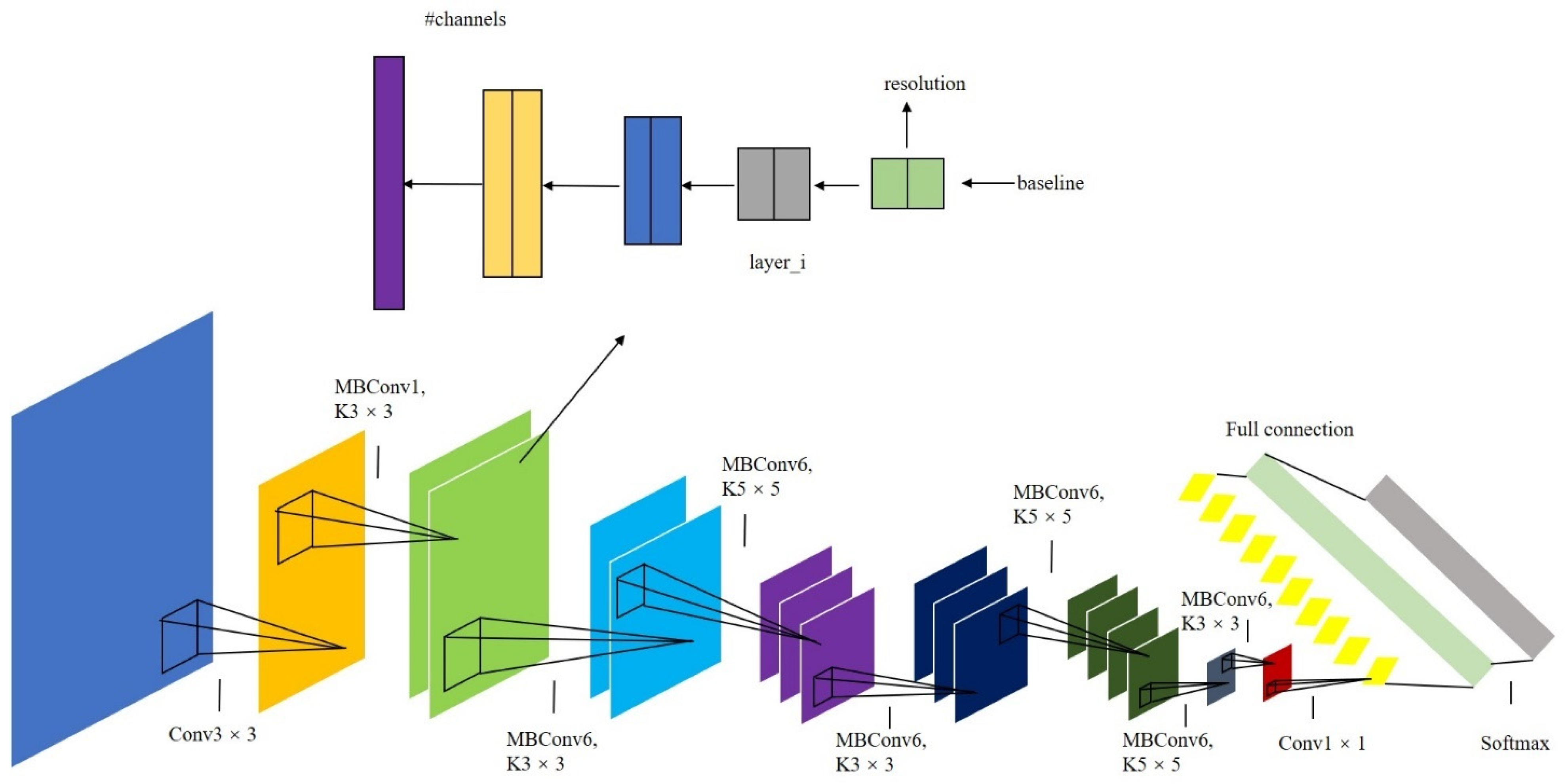
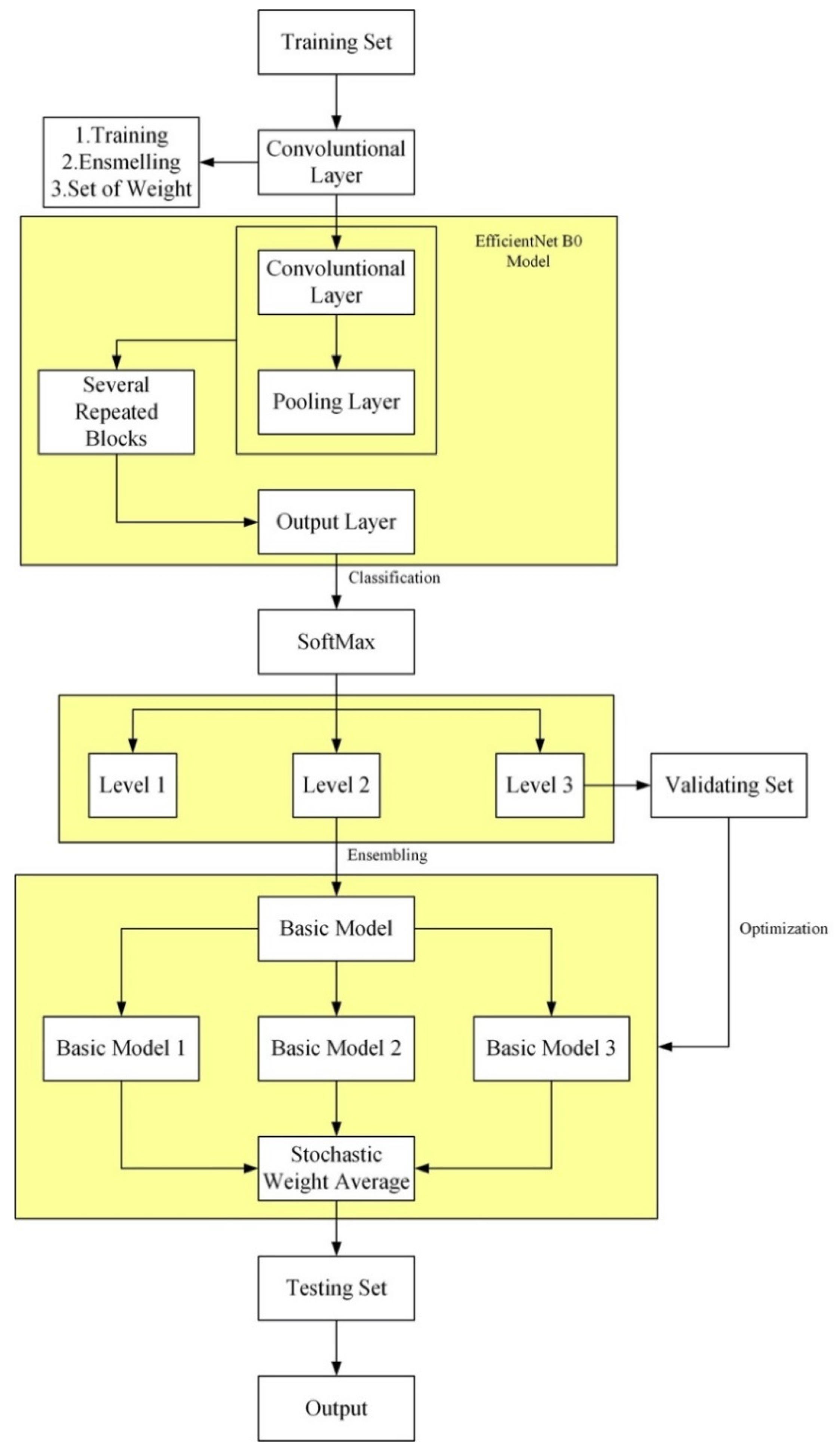
2.3.1. Application of EfficientNet

The impact of changes in atmospheric visibility on images is mainly reflected in the degradation of visual features such as image brightness, contrast, color, and scene depth. However, it is difficult to fully reflect the influence of the atmosphere on image formation based on only a few visual features [16]. Therefore, this paper applied the pre-trained deep neural network to visibility grading, followed by extracting the values through the network to train the neural network, thereby achieving the grading results. EfficientNet used composite coefficients to uniformly scale all dimensions of the model to achieve the highest accuracy and efficiency. The pre-trained EfficientNet was applied to the visibility grading model to effectively extract the abstract features and solve the problem of a small number of samples and uneven distribution of the visibility dataset.

In a traditional neural network training process, regardless of whether the recognition is correct or not, the classification error of each category is returned indiscriminately. The feedback parameter correction amount is small so that the parameter correction cannot be effectively expanded, and the network training convergence speed is reduced.

The definition of EfficientNet is [11]: designing a baseline network using neural architecture search and uniformly scaling all dimensions of depth, width, and resolution. The advantage of EfficientNet is that the design of the middle layer ensures that both its accuracy and efficiency are better than all previous convolutional networks, no matter whether the amount of data is large or small. This conclusion came from the experiment that was conducted in EfficientNet. According to results compared with other traditional neural networks, EfficientNet performs better than any other deep neural network in the case of the same amount of hyperparameters or the same number of layers.

EfficientNet was divided into eight structures of B0-B7 according to the depth of the model. Because the data and grading level in this research were relatively simple, EfficientNet-B0 was used as the baseline model. The architecture of EfficientNet is shown in Figure 5. Its main building block is mobile inverted bottleneck MBConv, to which the original researcher also adds squeeze-and-excitation optimization. To adapt EfficientNet to our research, a softmax layer was added at the end of the basic deep neural network model, which is used as a three-classification block to maintain our goals.

To be more specific, we utilized the image obtained in the field to describe the detailed procedure of our basic EfficientNet-B0 model. First, the images were obtained from our collective devices. Then it was reshaped to a 224 × 224 image with RGB channels. Later, the reshaped image would be transformed into other shapes with the help of the EfficientNet model, which is revealed in Figure 6. When all the steps were done, the matrix that was gained would be transported to the softmax layer.

2.3.2. Training Based on Softmax Regression Model

In order to establish the relationship between image features and visibility level, this paper used Softmax to establish the regression model [15,17]. The Softmax regression model is a generalization of the logistic regression model on multi-grading problems. In this paper, the class label $y_i$ represents the three visibility levels {Level 1, Level 2, Level 3}.

As shown in Figure 5 before, the simple three-classification model consists of a basic pretrained EfficientNet-B0 model and a softmax layer, whose output is three probability values (from 0 to 1). The probabilities corresponding to the three classifications are obtained by calculating matrix multiplication in the softmax layer. The criterion that the sum of these three probabilities is 1 is always true. If the output probability is [0, 0.14, 0.86], the input belongs to Level 3.

In the Softmax regression model, the training set consists of m labeled samples, as given by:

$$\left\{\left(x^{\left(1\right)},y^{\left(1\right)}\right),\dots ,\left(x^{\left(m\right)},y^{\left(m\right)}\right)\right\}$$

For a given test input x, a hypothesis function is used to estimate the probability value $p(y=j|x)$ for each category j, that is, estimating the probability of each classification result of x. The hypothesis function is going to output a k-dimensional vector to represent the k estimated probability values. In this paper, k = 3.

The Softmax classifier maps the input vector from N-dimensional space to the classification, and the result is given in the form of probability, as expressed by:

$$p_j=\frac{e^{\left({\theta }_k^{T_x}\right)}}{{{\displaystyle \sum }}_{k=1}^k{e}^{\left({\theta }_k^{T_x}\right)}} \left(j=1,2,\dots ,k\right)$$

(1)

where, ${\theta }_k={\left[{\theta }_{k1} {\theta }_{k2} {\theta }_{k3}\right]}^T$ is the weight value, which is the classification parameter corresponding to the category, and the total model parameter θ is expressed as:

$$\theta =\left[\begin{array}{c}{\theta }_1^T\\ {\theta }_2^T\\ {\theta }_3^T\end{array}\right]$$

(2)

The parameter θ is obtained by training the Softmax classifier. As a parameter, θ can calculate the probability of all possible categories of the item to be classified, and then the category to which it belongs can be determined. Given a dataset including m training samples $\left\{\left(x^{\left(1\right)},y^{\left(1\right)}\right),\dots ,\left(x^{\left(m\right)},y^{\left(m\right)}\right)\right\}$, where x represents the input vector, and y is the category label for each x. For a given test sample $x^{\left(i\right)}$, the Softmax classifier is used to estimate the probability that it belongs to each category. The form of the function $h_{\theta }\left(x\right)$ is expressed as:

$$h_{\theta }\left(x^{\left(i\right)}\right)=\frac{1}{{{\displaystyle \sum }}_{k=1}^k{e}^{\left({\theta }_k^{T_x\left(i\right)}\right)}}\left[\begin{array}{c}{e}^{\left({\theta }_1^{T_x\left(i\right)}\right)}\\ e^{\left({\theta }_2^{T_x\left(i\right)}\right)}\\ e^{\left({\theta }_3^{T_x\left(i\right)}\right)}\end{array}\right]$$

(3)

where, $h_{\theta }\left(x^{\left(i\right)}\right)$ is a vector whose element $p(y^{\left(i\right)}=j|x^{\left(i\right)}$; θ) represents the probability of $x^{\left(i\right)}$ belonging to category k, the sum of the elements in the vector is 1. For $x^{\left(i\right)}$, the k corresponding to the maximum probability value is selected as the grading result of the current image. The value of θ can be obtained from the cost function, which is defined as:

$$J\left(\theta \right)=\frac{1}{m}\left[{\displaystyle \sum }_{k=1}^k{\displaystyle \sum }_{k=1}^{k}T\{y^{\left(i\right)}=j\}log\frac{e^{\left({\theta }_k^{T_x\left(i\right)}\right)}}{{{\displaystyle \sum }}_{k=1}^k{e}^{\left({\theta }_k^{T_x\left(i\right)}\right)}}\right]$$

(4)

where, $T\left\{y^{\left(i\right)}=j\right\}$ is an indicative function, with 1 for true value and 0 for false value. By minimizing $J\left(\theta \right)$, the classifier parameter θ can be obtained.

A trained Softmax classifier is used in the image retrieval method to process each query image and feedback of its category.

2.3.3. Ensemble Learning

The traditional ensemble method is to ensemble several different models, then use the same input to predict the model, and then use some common method to determine the final grading result of the ensemble model [18,19]. In this paper, ensemble learning and deep learning are combined, and the final grading result can be produced by combining the gradings of multiple neural networks. Integrating the neural networks with different structures will get an excellent ensembled model. Because each model may make mistakes on different training samples, this ensemble method can maximize the model performance. The pretrained EfficientNet-B0 is substituted into Bagging for training, and 20 iterations are performed. The results are shown in

Table 3. The results of training by EfficientNet-B0 with 20 iterations.

Epoch	Time	Loss	ACC	Val_loss	Val_acc
1	35 s	0.6187	0.7303	1.3687	0.3429
2	17 s	0.3134	0.8939	6.2114	0.3571
3	19 s	0.2673	0.9212	6.6086	0.2429
4	18 s	0.3264	0.8848	0.0443	0.6714
5	19 s	0.2055	0.9152	1.3207	0.6143
6	16 s	0.2629	0.9242	0.2442	0.7143
7	16 s	0.2156	0.9394	2.6681	0.6857
8	17 s	0.1754	0.9303	1.4453	0.8143
9	17 s	0.1637	0.9364	0.1460	0.8429
10	16 s	0.0856	0.9818	1.0111	0.9000
11	16 s	0.1101	0.9727	0.0911	0.8286
12	16 s	0.1958	0.9394	1.6282	0.9000
13	16 s	0.0811	0.9818	0.6060	0.9286
14	16 s	0.0514	0.9939	0.0528	0.9429
15	16 s	0.0416	1.0000	0.1663	0.9286
16	16 s	0.0492	0.9939	0.0566	0.9429
17	16 s	0.0447	0.9939	0.8719	0.9286
18	16 s	0.0602	0.9879	0.4899	0.9286
19	16 s	0.0456	0.9970	0.0461	0.9429
20	11 s	0.0459	0.9970	0.4312	0.9286

.

The loss conforms to the expected convergence curve, indicating that the model fits well. After the training of EfficientNet-B0, the accuracy of the model is shown in Figure 7, and the final training result accuracy is close to 1, which indicates our model has a good performance in this grading task. By comparing the accuracy of each neural network, the last three networks are selected and ensembled by the SWA method as the training model for visibility grading.

2.3.4. Ensemble Method Based on Weight Space

SWA [12] is very close to the fast geometric ensemble (FGE), but its calculated loss is small. The SWA method is used in this paper to optimize the previous model obtained by ensemble learning.

The method ensembles the model by combining the same weights in different training stages, and then uses this ensemble model of combined weights to make gradings. Wilson et al. [20] proposed that the advantage of this method is that when combined weights are used, a model will be obtained after training, and this model can speed up the subsequent grading process. Experimental results show that this ensemble method of combined weights outperforms some popular snapshot ensembles (SE).

The working principle of SWA is as follows:

The first model is used to store the average of the model weights (W_SWA). The final model will be obtained after training and then is used for grading.

The second model is used to traverse the weight space (such as W in the equation) and explore using a recurrent learning rate. At the end of each learning rate period, the current weight of the second model is used to update the average weight of the model by weighting the average between the old average weight and the new set of weights in the second model.

$$W_{SWA}\leftarrow \frac{W_{SWA}·n_{models}+W}{n_{models}+1}$$

(5)

We utilized ensemble learning with the SWA method, which consists of three EfficientNet models with three discrepant groups of hyperparameters. A group of parameters is obtained in every training epoch in our training process, which is also recognized as an EfficientNet model. According to this method, the last three networks of Table 3 are selected, i.e., Epoch18, Epoch19, and Epoch20. Firstly, the three W_SWA models are stored in Epoch18, as Model 1, and the Epoch19 and Epoch20 networks are stored in memory as Model 2 during training. The average weight of Epoch18 and the new set of weights of the Epoch19 model are averaged to form the new Model 1. The above steps are repeated with the Epoch20 model. Finally, the atmospheric visibility grading model can be obtained using the three models through stochastic weights.

3. Results and Discussion

3.1. Experiment of Ensemble Learning Grading Based on SWA

In order to verify the effectiveness of the proposed method based on the EfficientNet and SWA algorithm, the cross-validation method was used to divide the training set and the validation set after obtaining the image dataset by the image acquisition device. A total of 2500 images with different visibility levels were used as the training set, and 500 images with different visibility levels were used as the verification set. In addition, 650 images with three approximate visibility ratios of 1:1:1 were used as the testing set, with the distribution of sample quantity shown in

Table 4. Account distribution of sample images in different visibility levels.

Visibility Level	Training Set	Test Set
Level 1	800	212
Level 2	850	218
Level 3	850	220

. The Jupyter Notebook software in Anaconda was used to build the SWA model based on EfficientNet and ensemble learning for training and testing based on Tensorflow and the Keras deep learning framework. Then the dataset was substituted into the SE model and FGE model, and a comparison was performed on the results. Our code will be made public on GitHub: https://github.com/ChristopherCao/An-Atmospheric-Visibility-Grading-Method-Based-on-Ensemble-Learning-and-Stochastic-Weight-Average (accessed on 20 June 2021).

In order to verify the accuracy of the grading results, images were substituted into the model to judge whether the grading result is consistent with the image name. They were consistent for correct grading, otherwise incorrect grading. For example, the grading result for file name 435 Level 3.png is Level 3. The real file name contains the substring of ‘Level 3’, and the grading is correct. Otherwise, the grading is false. The results are shown in Figure 8.

3.2. Evaluation Indicator

In this paper, the following indicators were set to verify the effect of deep neural network EfficientNet.

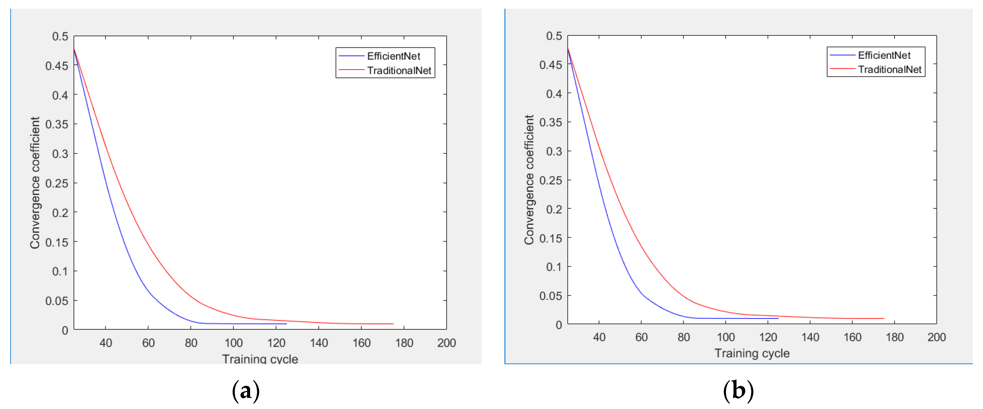
• Convergence coefficient: When the model training process ceased, the model training curve is regarded to tend to be stable with the increase of training times, then the model is considered to have converged. The equation is expressed by:

  $$E\ge \frac{1}{3}{\displaystyle \sum }_{i=n-2}^n|ac{c}_{i+1}-ac{c}_i|$$

  (6)

  where, $ac{c}_i$ refers to the accuracy in the training process, and E is a custom threshold.
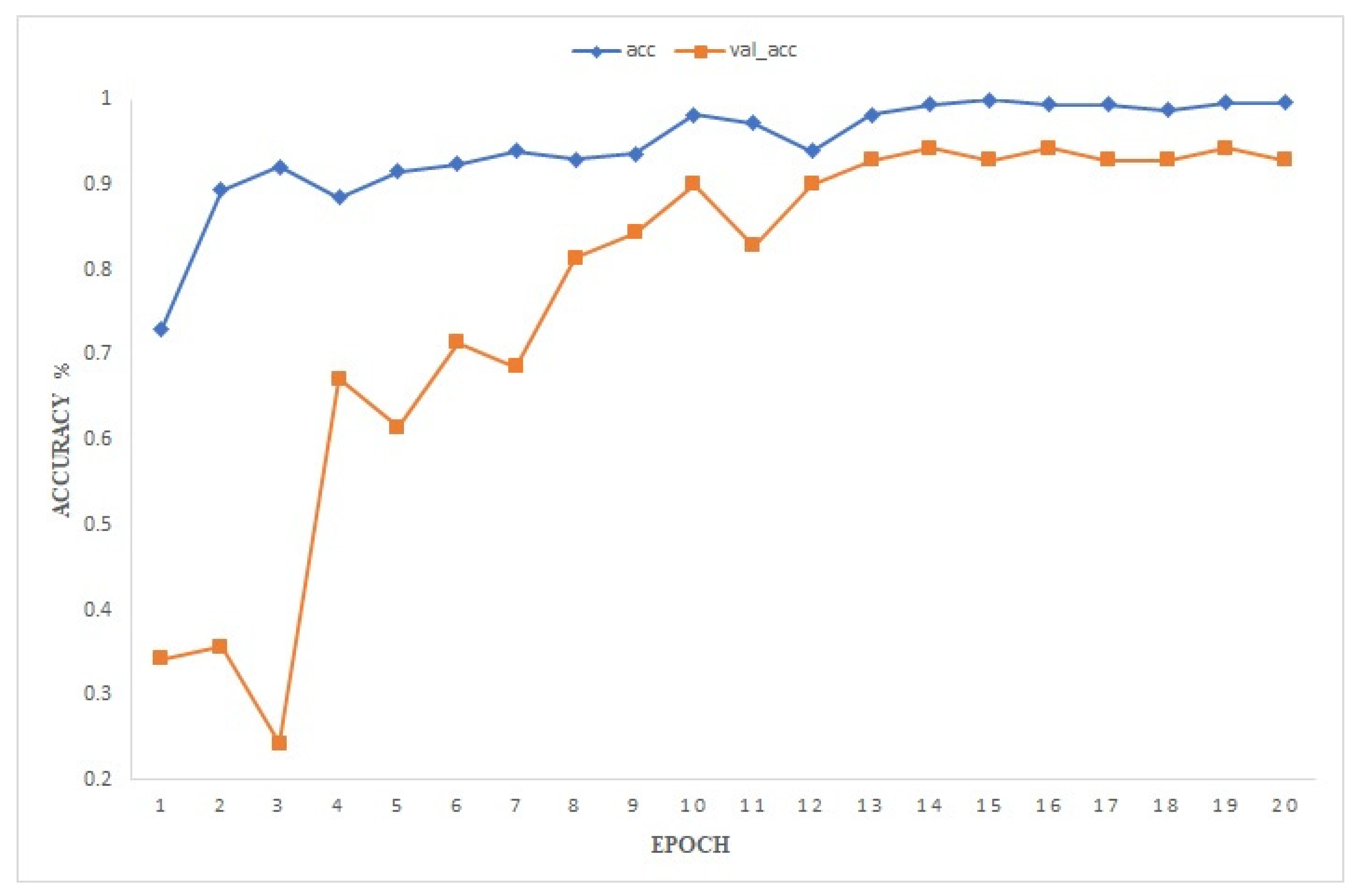
• Accuracy: There are many evaluation indicators to measure the model performance, and recognition accuracy is often used as the standard of model evaluation.

  $$ACC=\frac{TP+TN}{TP+TN+FN+FP}$$

  (7)

  where, TP represents a positive sample predicted by the model to be positive, TN represents a negative sample predicted by the model to be negative, FP represents a negative sample predicted by the model to be positive, and FN is a positive sample predicted by the model to be negative.

The traditional neural network feeds back the classification error to the hidden layer indiscriminately each time it is trained, so it cannot accurately strengthen the influence of the main component features on the network training. The EfficientNet algorithm can adjust the weight of the model according to the sample classification error, and then backpropagate to enhance or reduce the corresponding hidden layer parameters and bias to achieve the purpose of targeted training on the corresponding features, thereby effectively enhancing the main component. The influence of features on network training reduces the interference of invalid features on network training, continuously improves the accuracy of classification results, optimizes the convergence effect, and improves the sample recognition rate.

This section mainly analyzes the convergence and recognition effect of the EfficientNet algorithm. Analysis results show that the weight adjustment and integration model can improve the algorithm’s convergence, conduct training on large error characteristics, and improve classification accuracy. In order to further verify the application effect of the algorithm proposed in this article, the next chapter compares the EfficientNet algorithm with the same structure network algorithm.

3.3. Experiment Analysis

In order to verify the effectiveness of the model based on the visibility classification dataset, three factors, the convergence coefficient, model complexity, and accuracy, were evaluated, respectively. The specific settings were as follows to maintain the fairness of the experiment.

(1)

The EfficientNet and the algorithm of the traditional neural networks were tested twice utilizing a visibility dataset, and the number of iteration periods of the two algorithms under convergence conditions was compared and analyzed.

(2)

This method was compared with VGG19 [21], ResNet [22,23], and Senet [24] based on the visibility dataset. Repeated experiments were carried out to analyze the confusion matrix results of EfficientNet and other algorithms, as well as the overall recognition accuracy.

3.3.1. Convergence Analysis

According to the self-built dataset, the EfficientNet algorithm and the traditional neural network with the same structure were repeatedly trained twice, where the initial iteration period was set to 200 times. The number of training iteration times were compared when the two algorithms stop training. The curve between convergence indicator and training period was obtained through experimental analysis, as shown in Figure 9.

Figure 9 shows the training convergence curve of EfficientNet twice and the traditional network with the same structure. Figure 9a is the first training result. It can be seen from the figure that the EfficientNet training cycle reaches the convergence condition at about 80, then the training stops. The traditional network with the same structure needs to be trained for about 140 cycles to reach the convergence condition, then the training stops. Figure 9b is the second training result. It can be seen from the figure that the two training shows that EfficientNet basically reaches the convergence condition of about 80 when the training stops; the traditional neural network of the same structure needs to reach the convergence condition at about 130 iterations. Therefore, compared with the traditional neural network, the EfficientNet algorithm reaches the convergence condition 60 iterations earlier than the traditional neural network under the same conditions, indicating that the EfficientNet algorithm can effectively accelerate the convergence of the algorithm.

3.3.2. Overall Accuracy Analysis

In order to prove that this method is more suitable for visibility grading, the method was compared with VGG19, ResNet, and SEnet. Firstly, the whole sample training set was used as the model training data to construct the visibility recognition model. Then, the following five methods are verified by experiments based on the trained visibility recognition model. Finally, five repeated experimental results of EfficientNet, VGG19, ResNet, and SEnet under the overall sample were acquired through experimental comparison. The experimental results are shown in Figure 10.

Figure 10 also demonstrates the results of five experiments of EfficientNet, VGG19, ResNet, and SEnet. According to the figure, the five-times recognition accuracy of EfficientNet is about 90%. The recognition accuracy of VGG19 is about 73%, the recognition accuracy of SEnet is about 80%, and the recognition accuracy of ResNet is about 76%. According to the experimental results, several algorithms have good stability and low volatility for mass fog visibility recognition. Therefore, EfficientNet has a high accuracy, which shows that the algorithm in this paper can solve the slow training speed of large-scale data and maintain a high recognition effect.

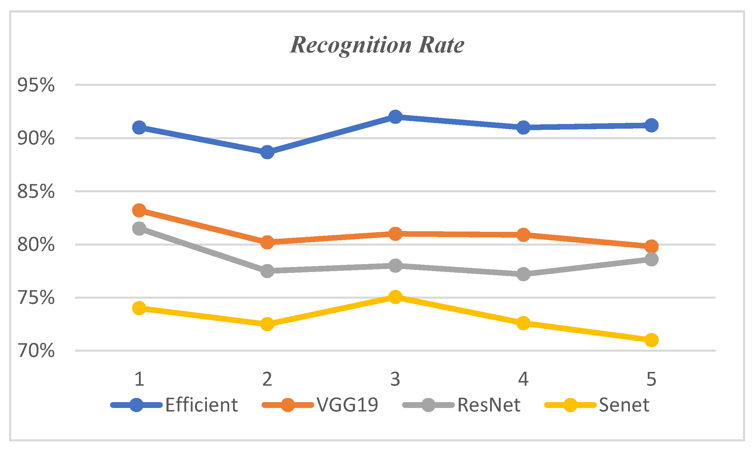
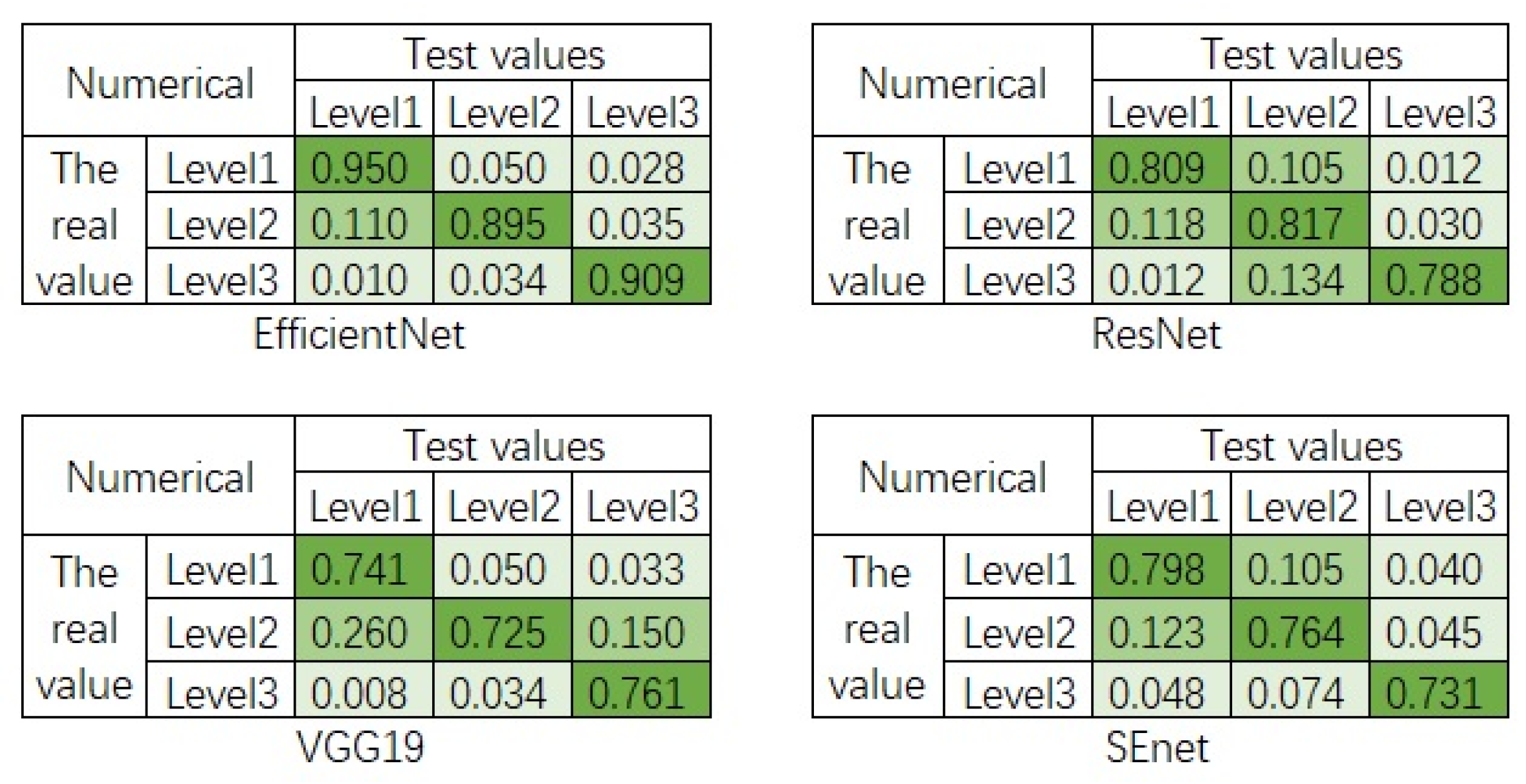
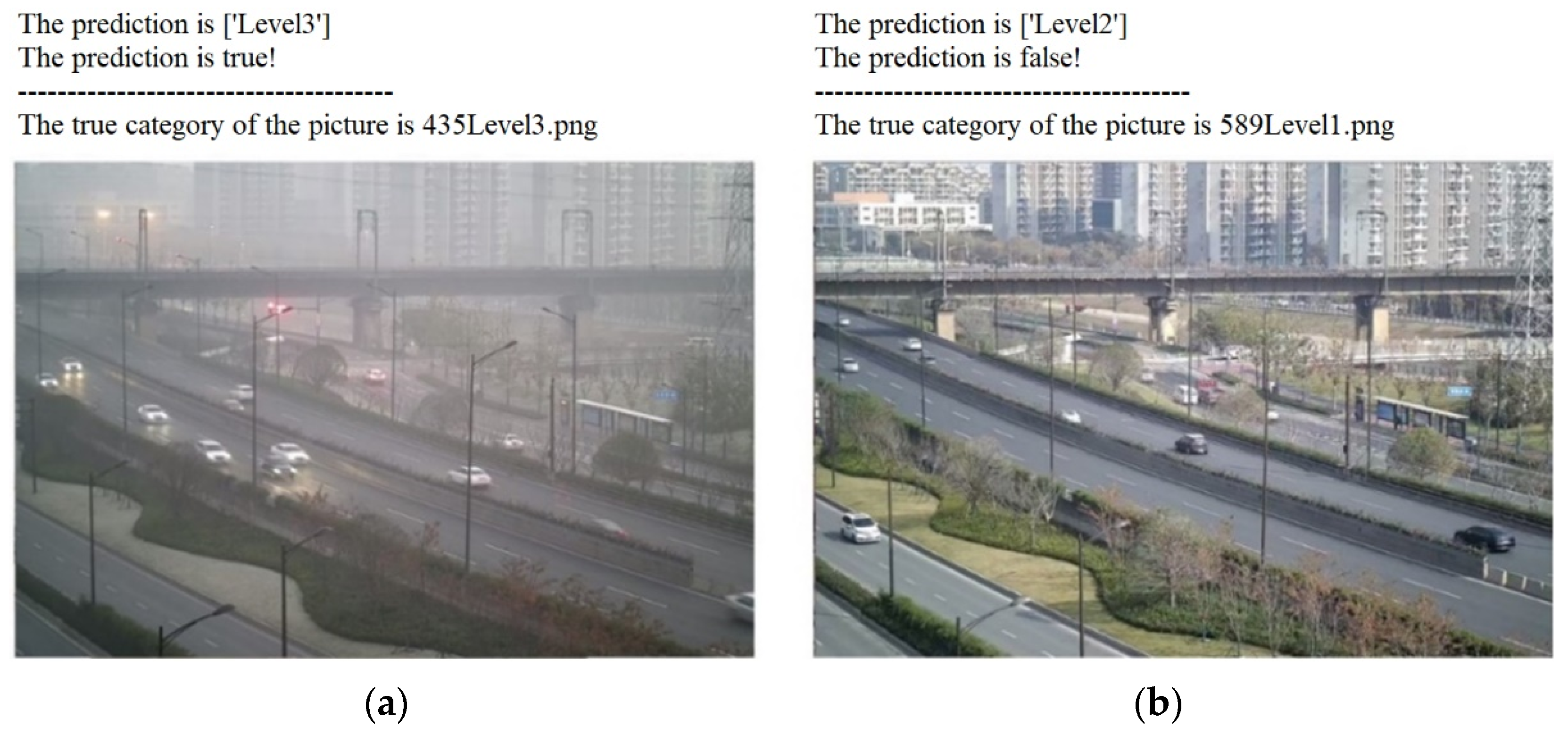
3.3.3. Analysis of Recognition Accuracy

In the experiment, the overall sample set was applied to train the model, and the performance of the model was analyzed according to the recognition results of each visibility level test set. Firstly, the training set was input to construct the visibility recognition model. Then, the corresponding mass fog visibility level test set was used to verify based on the trained visibility detection model. Finally, the identification results of EfficientNet, VGG19, ResNet, and SEnet under each level were obtained by comparison.

It can be seen from Figure 11 that the recognition accuracy of EfficientNet at three visibility levels reaches 95.00%, 89.45%, and 90.91%, respectively, and the recognition accuracy rate is above 90%. The recognition accuracy rate at different visibility levels is higher than that of VGG19, ResNet, and SEnet, indicating that EffcientNet has high recognition accuracy.

In addition, it can be seen from Figure 11 of the confusion matrix that EfficientNet is better than VGG19, ResNet, and SEnet in the recognition accuracy of each level. It shows that EfficientNet can recognize the visibility level of mass fog well under the condition of accelerating the operation speed, which meets the requirements of real-time monitoring of an expressway.

4. Conclusions

(1)

At present, deep learning has been widely used in the field of image processing, and it is easy to operate and has considerably high accuracy among many methods, which has received extensive attention from researchers. Particularly, EfficientNet is a deep neural network model that can be applied to small datasets and maintain high accuracy. It has shown good performance on the image datasets we collected in the experiment.

(2)

The SWA method ensures that the model can converge faster during the training process. On the other hand, it achieves the self-ensemble of the deep learning model, that is, the deep neural network with the same model architecture, but different weights are ensembled. Therefore, the detection accuracy is significantly improved.

(3)

An atmospheric visibility detection model based on EfficientNet and ensemble learning has been built in this paper. Three atmospheric visibility levels can be detected and classified by training a deep learning model and integrating the obtained deep neural network with the same model architecture but different model weights. According to the performance of the model in the experiment, it can be concluded that the detection accuracy of the three atmospheric visibility levels of Level 1, Level 2, and Level 3 are 95.00%, 89.45%, and 90.91%, respectively, with an average detection rate of 91.79%. The model proposed in this paper can more accurately grade atmospheric visibility. In addition, the proposed method can only maintain high accuracy in an experimental environment with good light characteristics, and the experimental data set needs to be further improved.

References

1. Palvanov, A.; Cho, Y.I. Visnet: Deep convolutional neural networks for forecasting atmospheric visibility. Sensors 2019, 19, 1343. [Google Scholar] [CrossRef] [PubMed] [Green Version]
2. Park, S.; Lee, D.H.; Kim, Y.G. In Development of a transmissometer for meteorological visibility measurement. In Proceedings of the 2015 Conference on Lasers and Electro-Optics Pacific Rim, Busan, Korea, 24–28 August 2015. [Google Scholar]
3. Hautiére, N.; Babari, R.; Dumont, É.; Brémond, R.; Paparoditis, N. In Estimating meteorological visibility using cameras: A probabilistic model-driven approach. In Proceedings of the Asian Conference on Computer Vision, Queenstown, New Zealand, 8–12 November 2010. [Google Scholar]
4. Song, H.; Gao, Y.; Chen, Y. Traffic estimation based on camera calibration visibility dynamic. Chin. J. Comput. 2015, 38, 1172–1187. [Google Scholar]
5. Chen, A.; Xia, J.; Chen, Y.; Tang, L. Research on visibility inversion technique based on digital photography. Comput. Simul. 2018, 35, 252–256. [Google Scholar]
6. Tang, S.; Li, Q.; Hu, L.; Ma, Q.; Gu, D. A visibility detection method based on transfer learning. Comput. Eng. 2019, 45, 242–247. [Google Scholar]
7. Bosse, S.; Maniry, D.; Muller, K.R.; Wiegand, T.; Samek, W. Deep neural networks for no-reference and full-reference image quality assessment. IEEE Trans. Image Process. 2018, 27, 206–219. [Google Scholar] [CrossRef] [PubMed] [Green Version]
8. You, Y.; Lu, C.; Wang, W.; Tang, C.K. Relative CNN-RNN: Learning relative atmospheric visibility from images. IEEE Trans. Image Process. 2019, 28, 45–55. [Google Scholar] [CrossRef] [PubMed]
9. Graves, N.; Newsam, S. Camera-based visibility estimation: Incorporating multiple regions and unlabeled observations. Ecol. Inform. 2014, 23, 62–68. [Google Scholar] [CrossRef]
10. Zheng, N.; Luo, M.; Zou, X.; Qiu, X.; Lu, J.; Han, J.; Wang, S.; Wei, Y.; Zhang, S.; Yao, H. A novel method for the recognition of air visibility level based on the optimal binary tree support vector machine. Atmosphere 2018, 9, 481. [Google Scholar] [CrossRef] [Green Version]
11. Tan, M.; Le, Q.V. In Efficientnet: Rethinking model scaling for convolutional neural networks. In Proceedings of the 36 th International Conference on Machine Learning, Long Beach, CA, USA, 9–15 June 2019. [Google Scholar]
12. Chen, Y.; Kang, X.; Shi, Y.Q.; Wang, Z.J. A multi-purpose image forensic method using densely connected convolutional neural networks. J. Real-Time Image Process 2019, 16, 725–740. [Google Scholar] [CrossRef]
13. Xiang, W.; Xiao, J.; Wang, C.; Liu, Y. In A new model for daytime visibility index estimation fused average Sobel gradient and dark channel ratio. In Proceedings of the 2013 3rd International Conference on Computer Science and Network Technology, Dalian, China, 12–13 October 2013. [Google Scholar]
14. Chaabani, H.; Werghi, N.; Kamoun, F.; Taha, B.; Outay, F. Estimating meteorological visibility range under foggy weather conditions: A deep learning approach. Proced. Comput. Sci. 2018, 141, 478–483. [Google Scholar] [CrossRef]
15. Yao, Y.; Wang, H. Optimal subsampling for softmax regression. Stat. Pap. 2019, 60, 235–249. [Google Scholar] [CrossRef]
16. Cheng, X.; Yang, B.; Liu, G.; Olofsson, T.; Li, H. A total bounded variation approach to low visibility estimation on expressways. Sensors 2018, 18, 392. [Google Scholar]
17. Alhichri, H.; Bazi, Y.; Alajlan, N.; Bin Jdira, B. Helping the visually impaired see via image multi-labeling based on squeezenet CNN. Appl. Sci. 2019, 9, 4656. [Google Scholar] [CrossRef] [Green Version]
18. Lu, Z.; Xia, J.; Wang, M.; Nie, Q.; Ou, J. Short-term traffic flow forecasting via multi-regime modeling and ensemble learning. Appl. Sci. 2020, 10, 356. [Google Scholar] [CrossRef] [Green Version]
19. Zheng, C.; Wang, C.; Jia, N. An ensemble model for multi-level speech emotion recognition. Appl. Sci. 2019, 10, 205. [Google Scholar] [CrossRef] [Green Version]
20. Izmailov, P.; Podoprikhin, D.; Garipov, T.; Vetrov, D.; Wilson, A.G. In Averaging weights leads to wider optima and better generalization. In Proceedings of the 34th Conference on Uncertainty in Artificial Intelligence, Monterey, CA, USA, 6–10 August 2018. [Google Scholar]
21. Long, M.; Zhu, H.; Wang, J.; Jordan, M.I. In Deep transfer learning with joint adaptation networks. In Proceedings of the 34th International Conference on Machine Learning, Sydney, Australia, 6–11 August 2017. [Google Scholar]
22. Wu, Z.; Shen, C.; Hengel, A.V.D. Wider or deeper: Revisiting the ResNet model for visual recognition. Pattern Recognit. 2019, 90, 119–133. [Google Scholar] [CrossRef] [Green Version]
23. Szegedy, C.; Ioffe, S.; Vanhoucke, V.; Alemi, A.A. In Inception-v4, inception-ResNet and the impact of residual connections on learning. In Proceedings of the Thirty-First AAAI Conference on Artificial Intelligence, San Francisco, CA, USA, 4–9 February 2017. [Google Scholar]
24. Hu, J.; Shen, L.; Albanie, S.; Sun, G.; Wu, E. Squeeze-and-Excitation Networks. IEEE Trans. Pattern Anal. Mach. Intell. 2019, 42, 2011–2023. [Google Scholar] [CrossRef] [PubMed] [Green Version]
Figure 1. Overview of image acquisition device with 1. case, 2. screen, 3. control host, 4. camera, 5. computer, 6. WIFI, 7. solar battery.
Atmosphere 12 00869 g001
Figure 2. Part of the acquired visibility images and their corresponding air quality: (a) good, (b) moderate, (c) poor.
Atmosphere 12 00869 g002
Figure 3. Flow chart of atmospheric visibility classification.
Atmosphere 12 00869 g003
Figure 4. The flow chart of visibility level grading is based on deep neural network EfficientNet and ensemble learning upon stochastic weight average.
Atmosphere 12 00869 g004
Figure 5. Schematic diagram of the simple three-classification networks and the classification process.
Atmosphere 12 00869 g005
Figure 6. Feature extraction using a pre-trained EfficientNet-B0 baseline network model.
Atmosphere 12 00869 g006
Figure 7. Accuracy of the model. The blue curse represents the accuracy of the performance on the model training set. The orange one shows the accuracy of the validation set.
Atmosphere 12 00869 g007
Figure 8. The model grading and determination instance: (a) The result of the model grading is consistent with the file name and the judgment is correct; (b) The result of the model grading is inconsistent with the file name, and the judgment is false.
Atmosphere 12 00869 g008
Figure 9. Convergence curve comparison chart: (a) the first training convergence curve; (b) the second training convergence curve.
Atmosphere 12 00869 g009
Figure 10. The recognition accuracy of each neural network, including EfficientNet, VGG19, ResNet, and SEnet.
Atmosphere 12 00869 g010
Figure 11. The confusion matrix diagram of the recognition results of each network.
Atmosphere 12 00869 g011