
Atlantic Niño/Niña Prediction Skills in NMME Models


Abstract
1. Introduction
2. Models and Data
3. Results
3.1. An Overview of the Atlantic Niño/Niña Prediction Skill in the Deterministic Sense
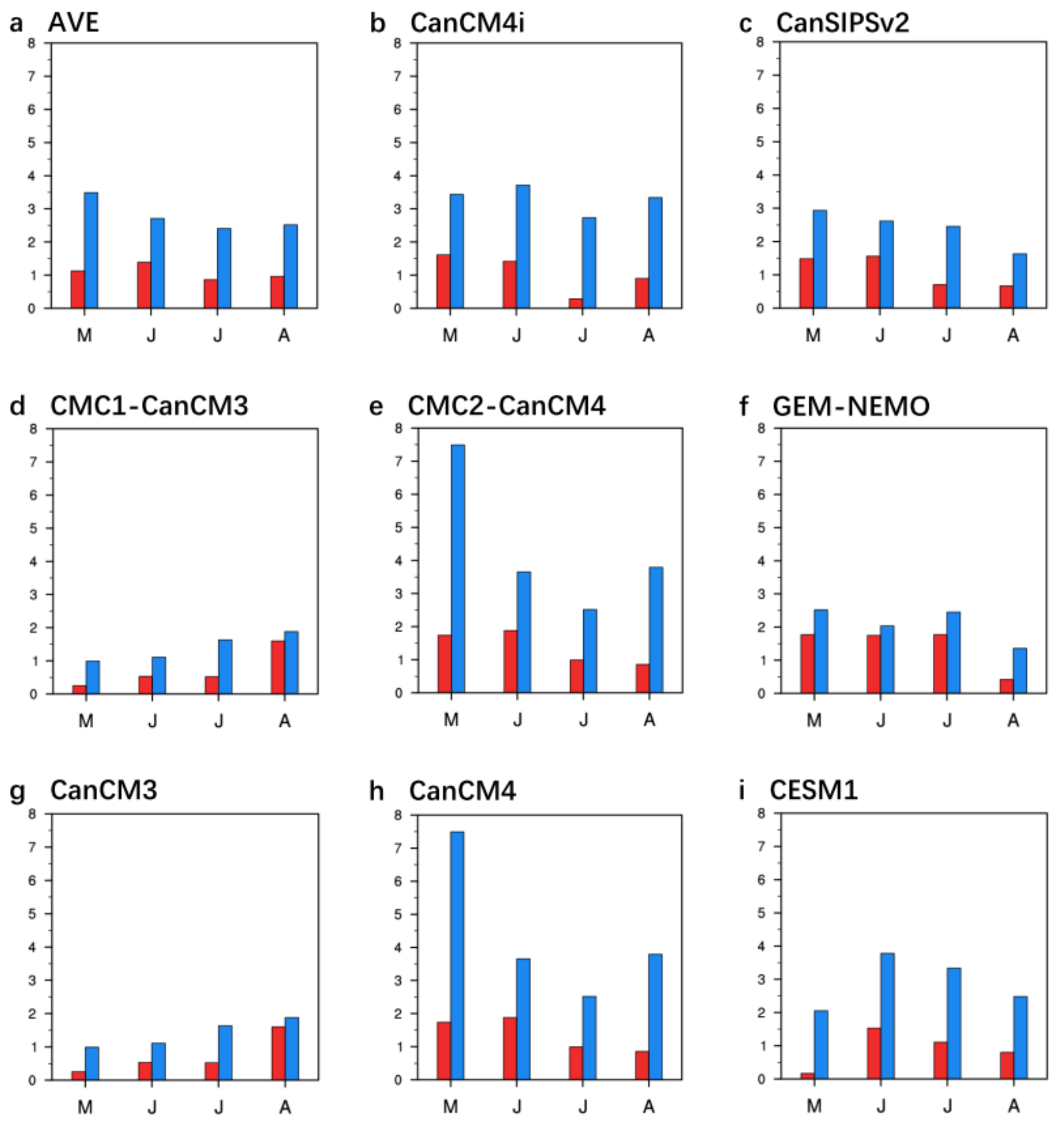
3.2. Seasonal Dependence of the Atlantic Niño/Niña Prediction Skill
3.3. Comparisons for the Atlantic Niño and Niña Prediction Skills
3.4. Overall Probability Forecast Skill
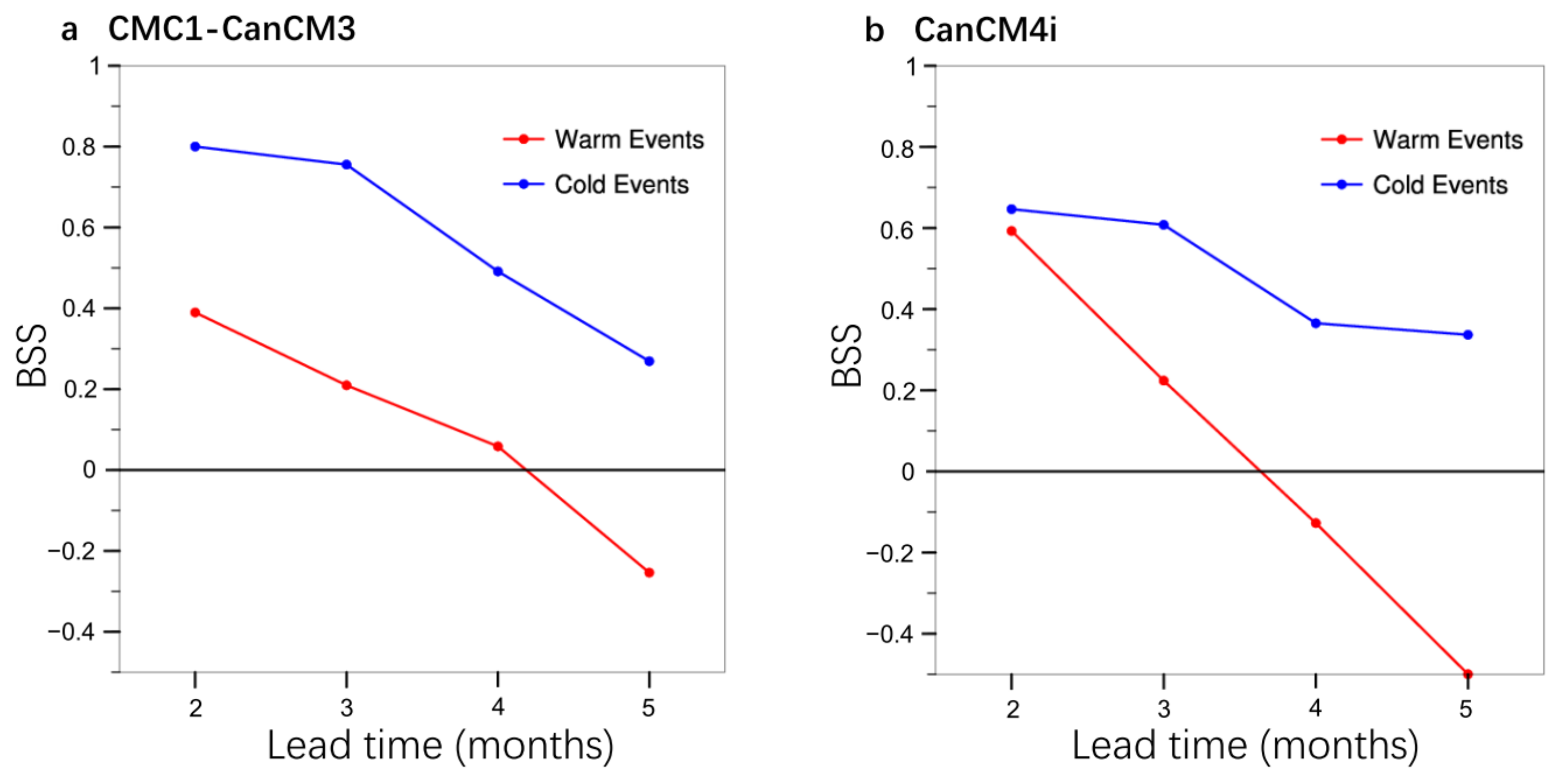
3.4.1. BSS
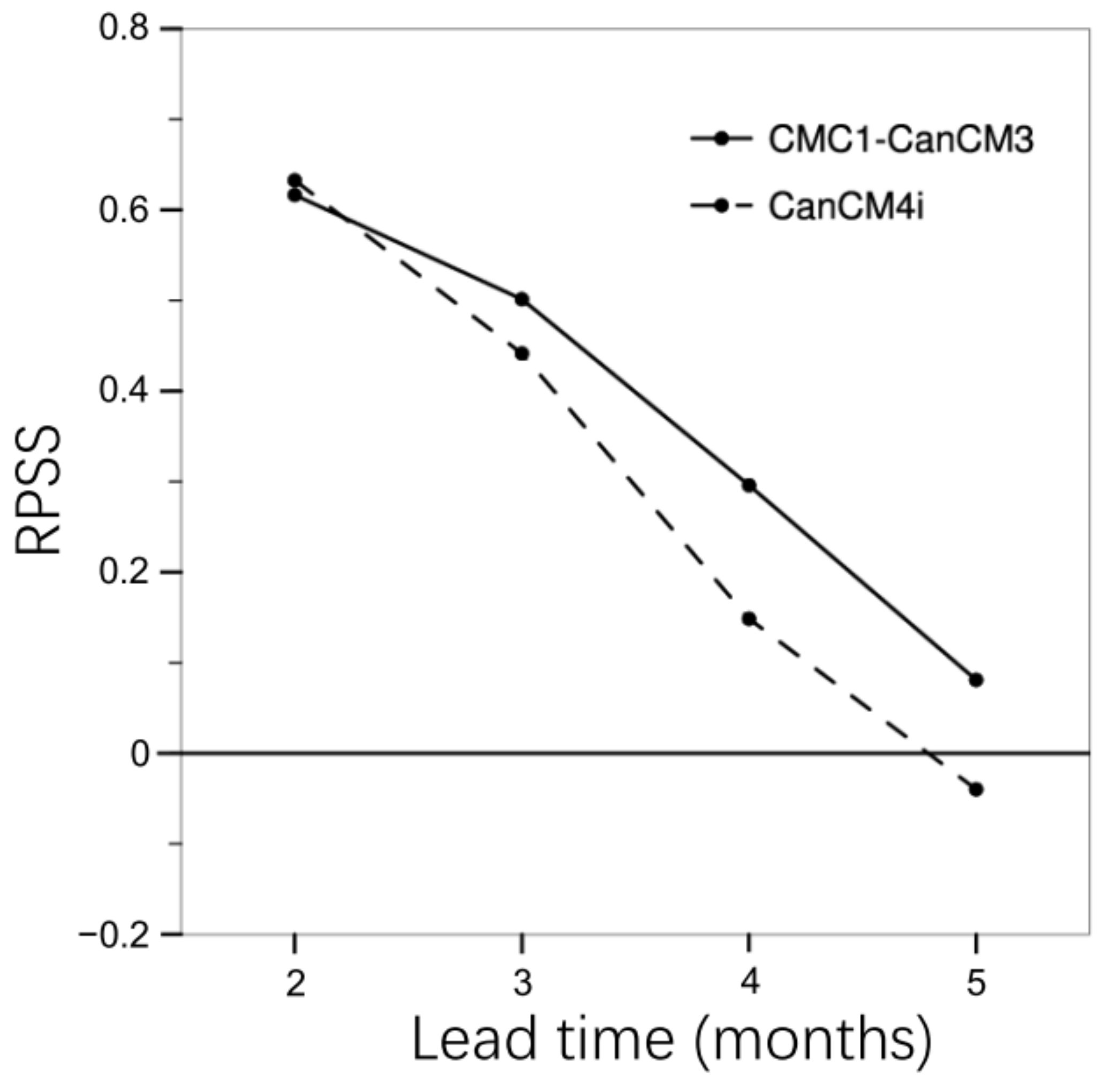
3.4.2. RPSS
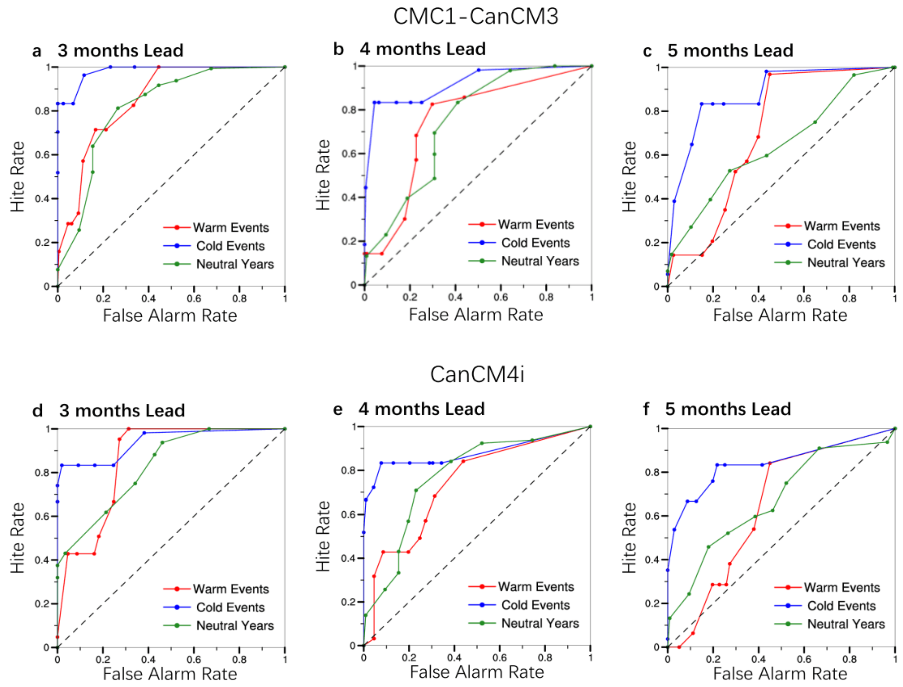
3.4.3. ROC
4. Possible Factors Responsible for the Atlantic Niño/Niña Forecast Errors
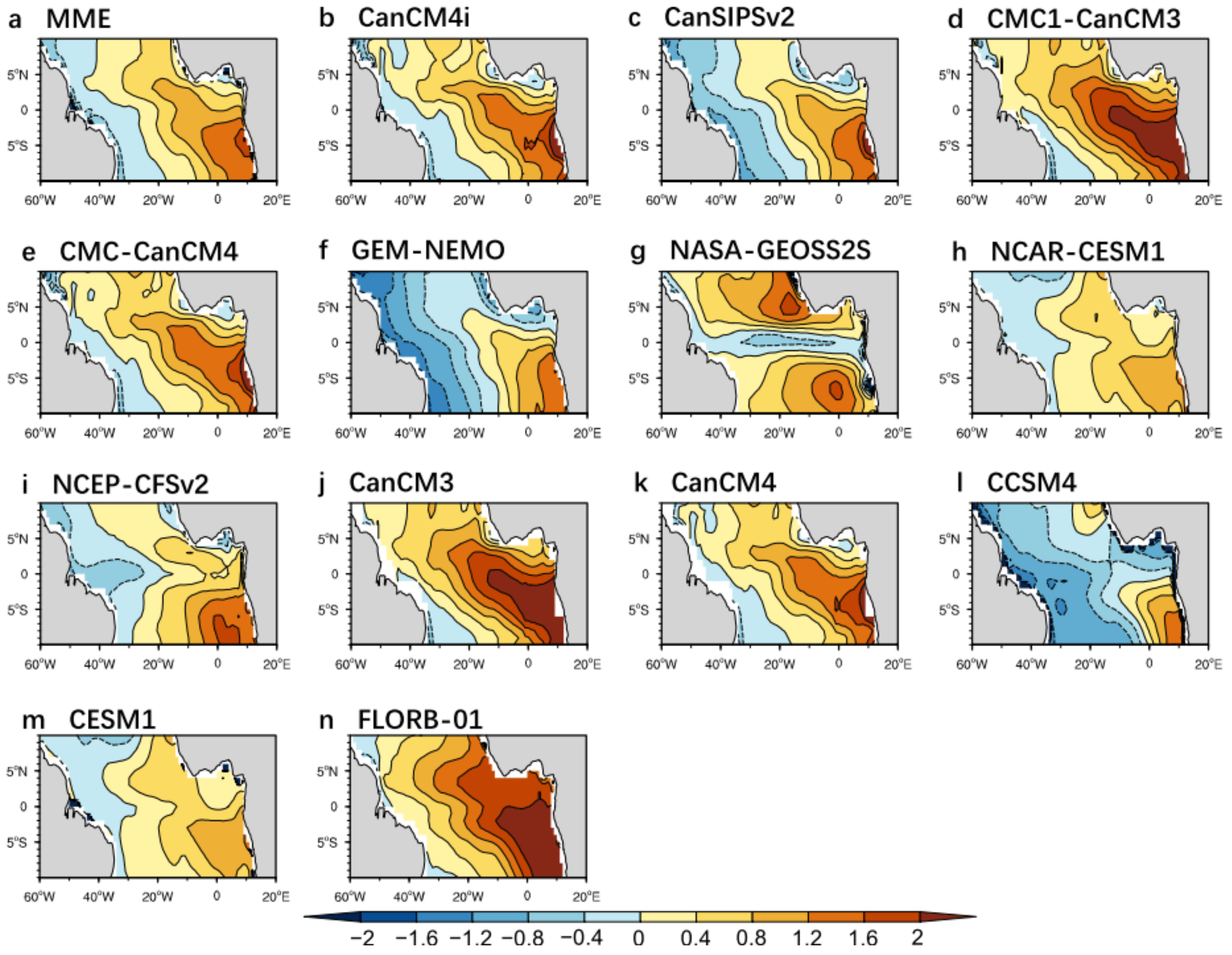
4.1. Mean State Biases in Equatorial Atlantic Sector
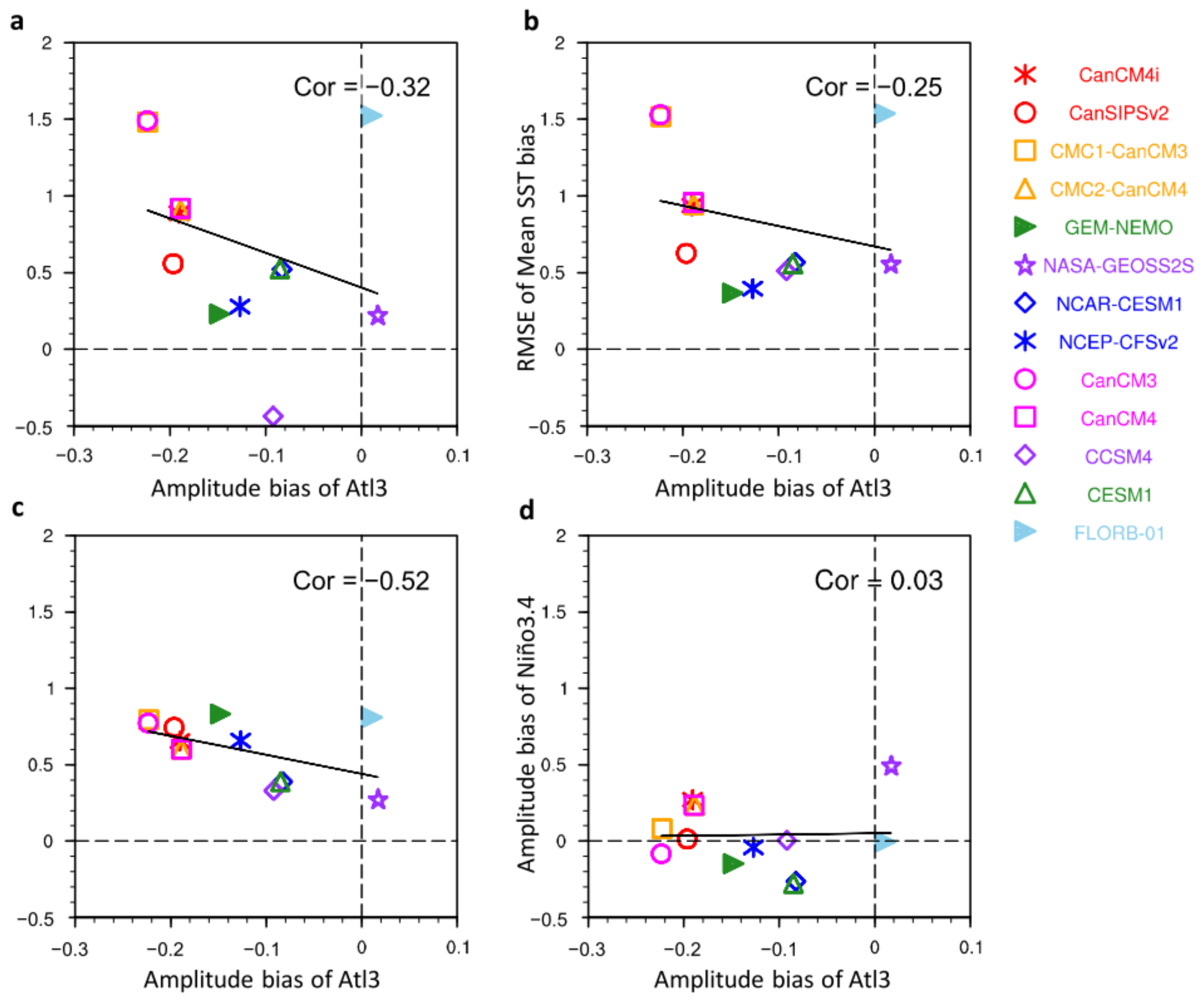
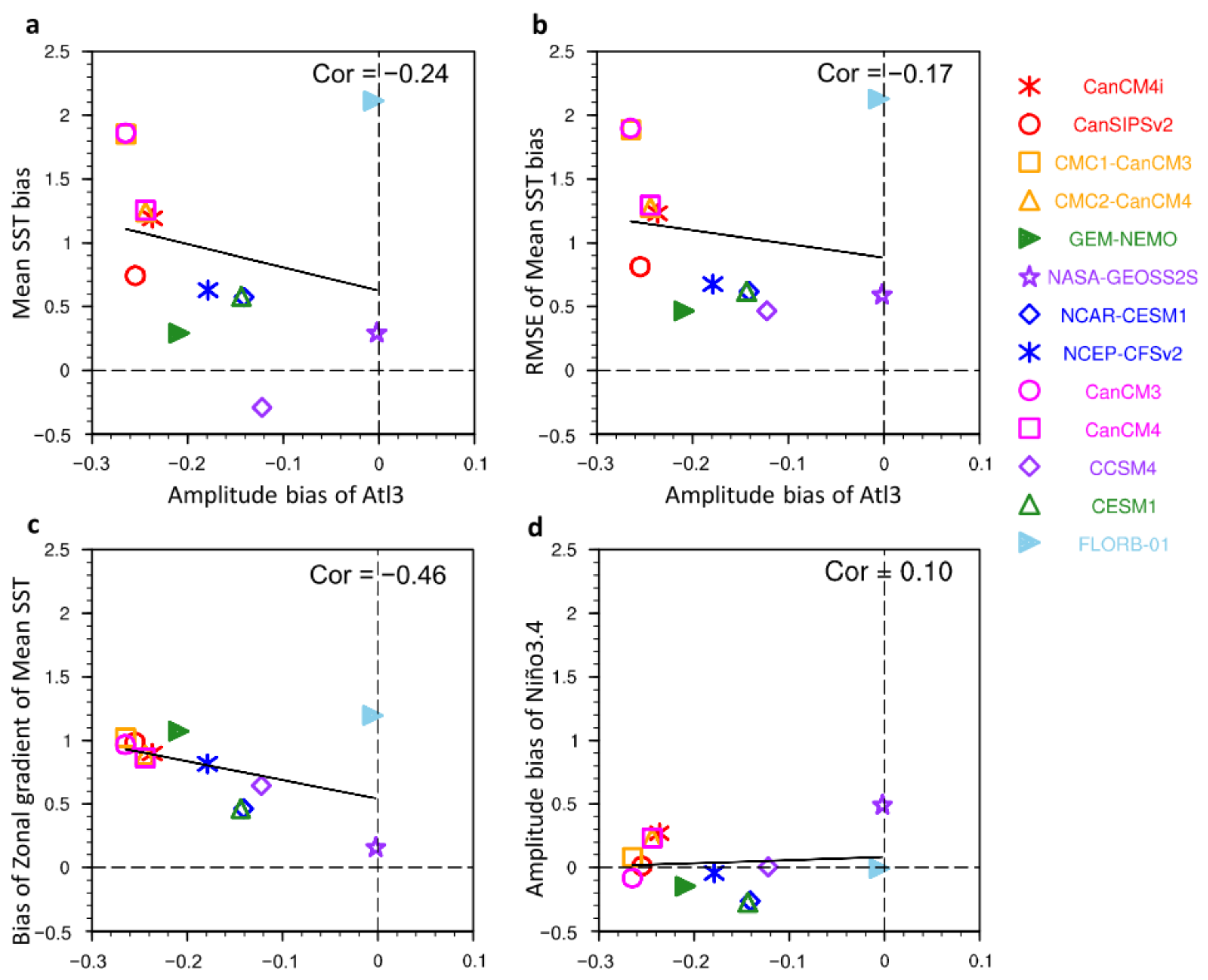
4.2. Factors Responsible for the Amplitude Bias of Atlantic Niño/Niña Prediction
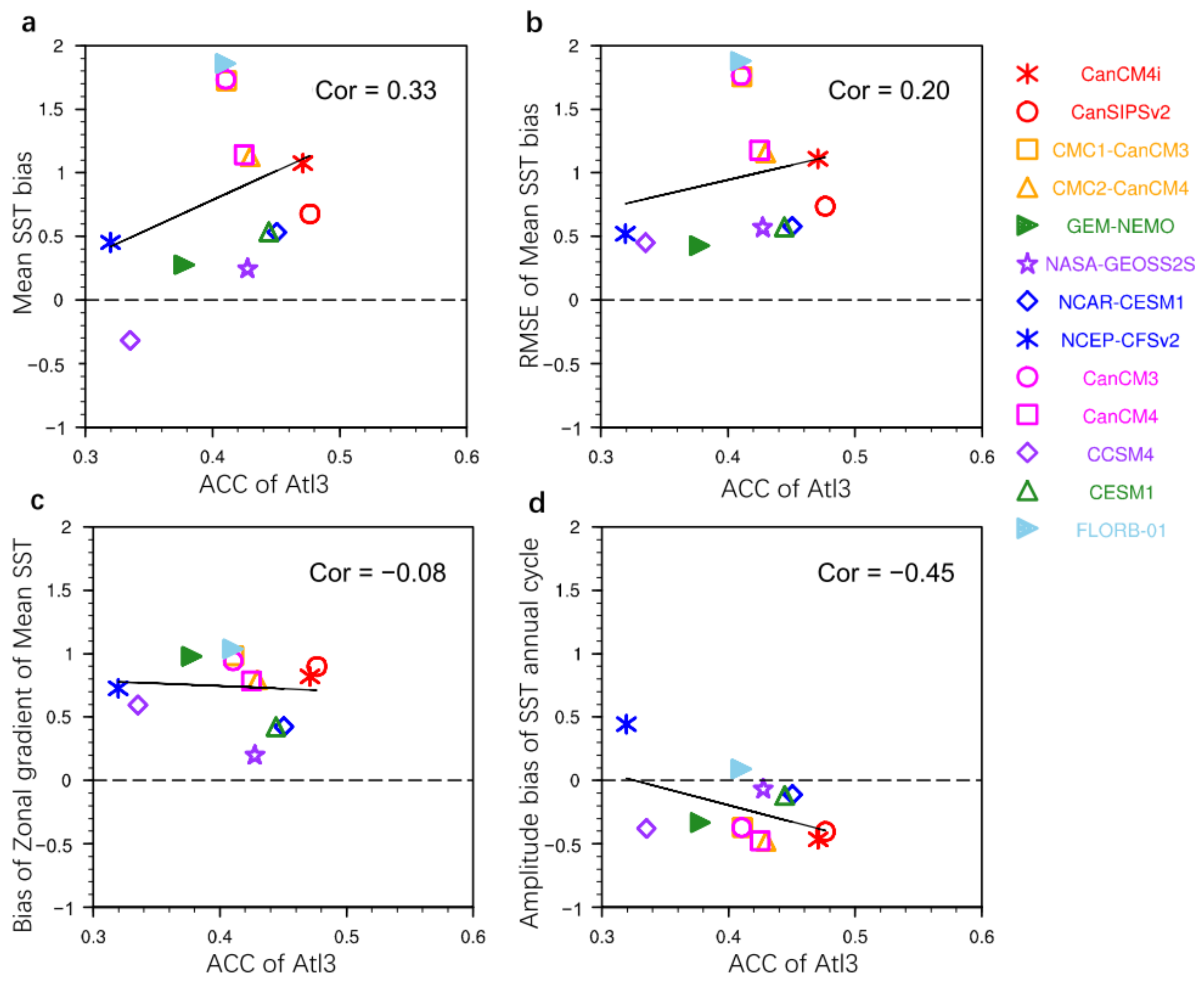
4.3. Factors Responsible for the Prediction Skills Based on ACC
5. Conclusions
- (1)
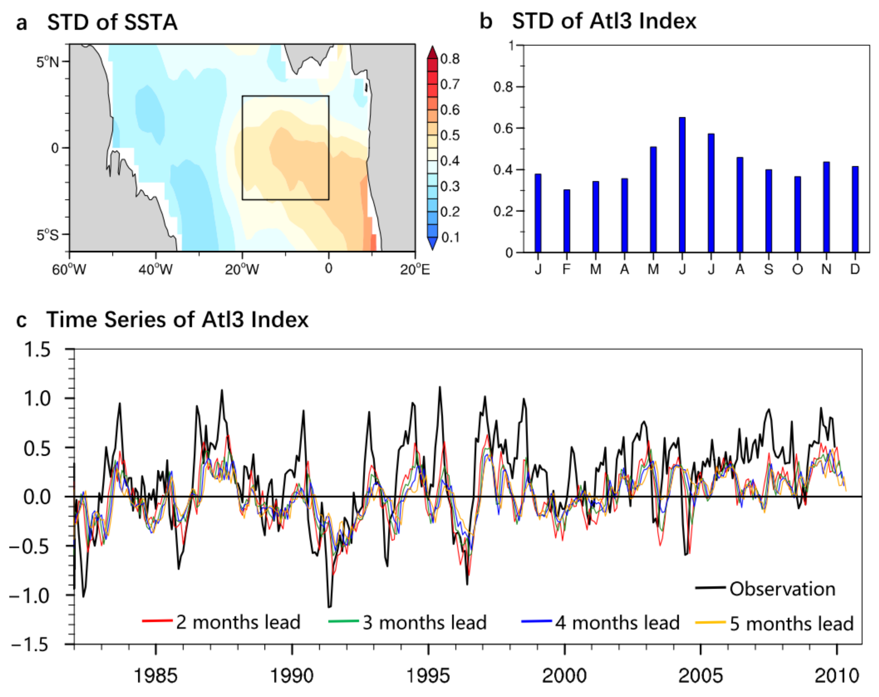
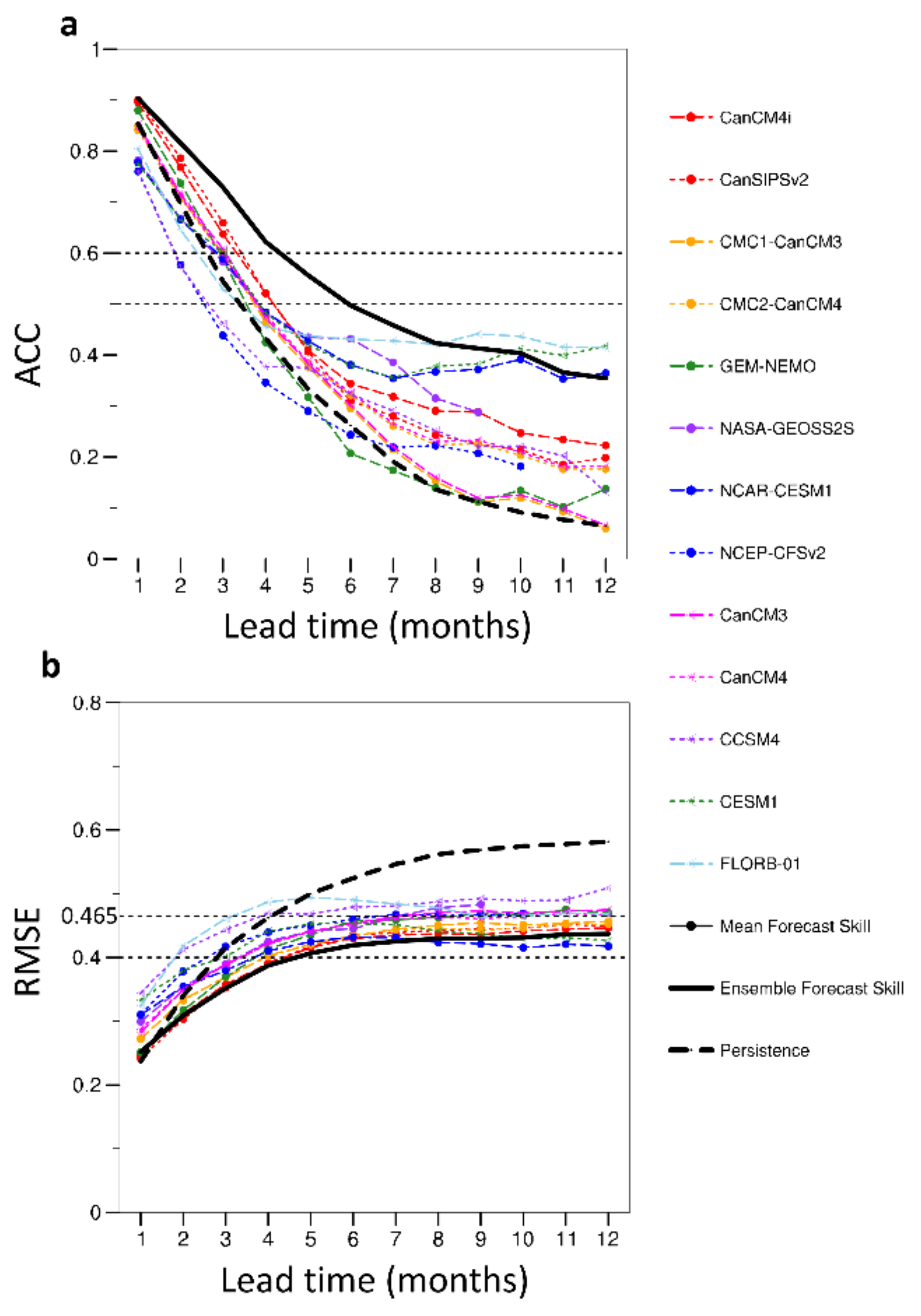
- Almost all the NMME models have underestimated the amplitude of Atlantic Niño/Niña, and the amplitude bias generally increases with the increasing lead time. From the perspective of the individual models, the prediction skill of Atlantic Niño/Niña for the majority of the NMME models can reach three months. Specifically, most of the models are capable to predict Atlantic Niño/Niña at three-month-lead with the RMSE less than 0.4. Particularly, four models (CanCM4i, CanSIPSv2, CMC1-CanCM3, and CMC2-CanCM4) show the RMSE results below 0.4 at 4-month-lead. When one STD of the observed Atl3 index is chose as the threshold value, most of the models have the ability to predict Atl3 index at seven-month-lead or even 12-month-lead. When 0.6 is chose as the cut off value for ACC, the prediction skills in half of the NMME models can reach three months. Among the NMME models, CanCM4i and CanSIPSv2 show the best skill in predicting Atlantic Niño/Niña. Two representative models are selected for further assessing the prediction skill in a probabilistic sense. The results based on the probabilistic measures (BSS, RPSS and ROC) agree with each other, and are generally consistent with those based on the deterministic measures.
- (2)
- The MME made by the NMME models shows better prediction skills than any of individual models. Specifically, the prediction skill for the MME reaches 6 (more than 4) months when 0.5 (0.6) is chose as the cut off value for ACC. As to the RMSE, the MME result keeps far below one STD of the observed Atl3 index for even 12-month-lead forecast, and the prediction skill for the MME result can reach nearly five months when 0.4 is chose as the threshold value. Therefore, the prediction skill for the MME can reach around five months, indicating that the MME method is an effective approach for reducing forecast errors.
- (3)
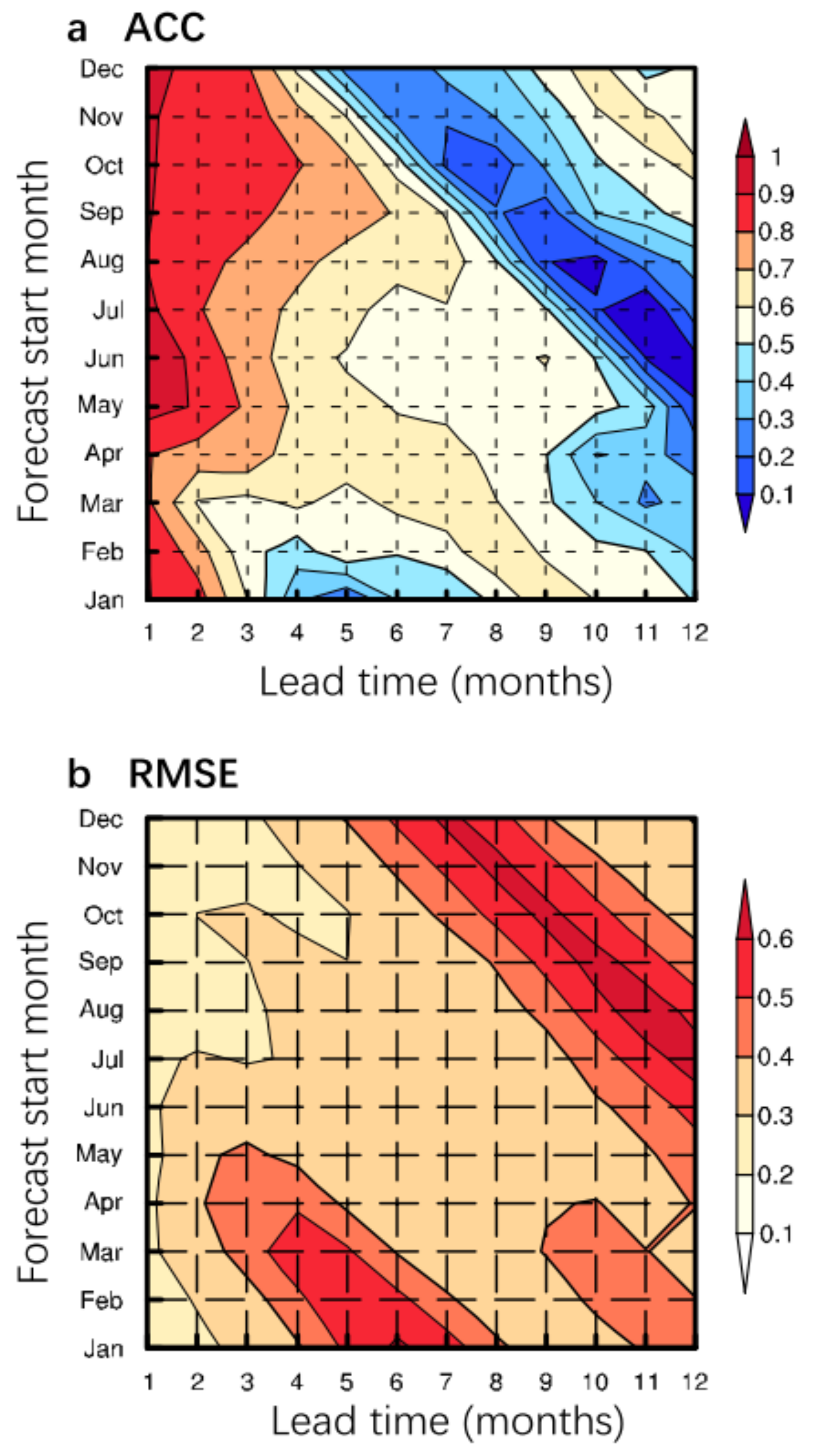
- It is further found that the prediction skill of Atlantic Niño/Niña shows clear seasonality. Both ACC and RMSE results show that the prediction skill of Atlantic Niño/Niña generally reaches more than six months for the forecasts starting from May to November, but is limited within four months for the forecasts starting in boreal winter. As the prediction skill shows a marked dip across the boreal spring, it is suggested that the prediction of Atlantic Niño/Niña in NMME models suffers a “spring predictability barrier”.
- (4)
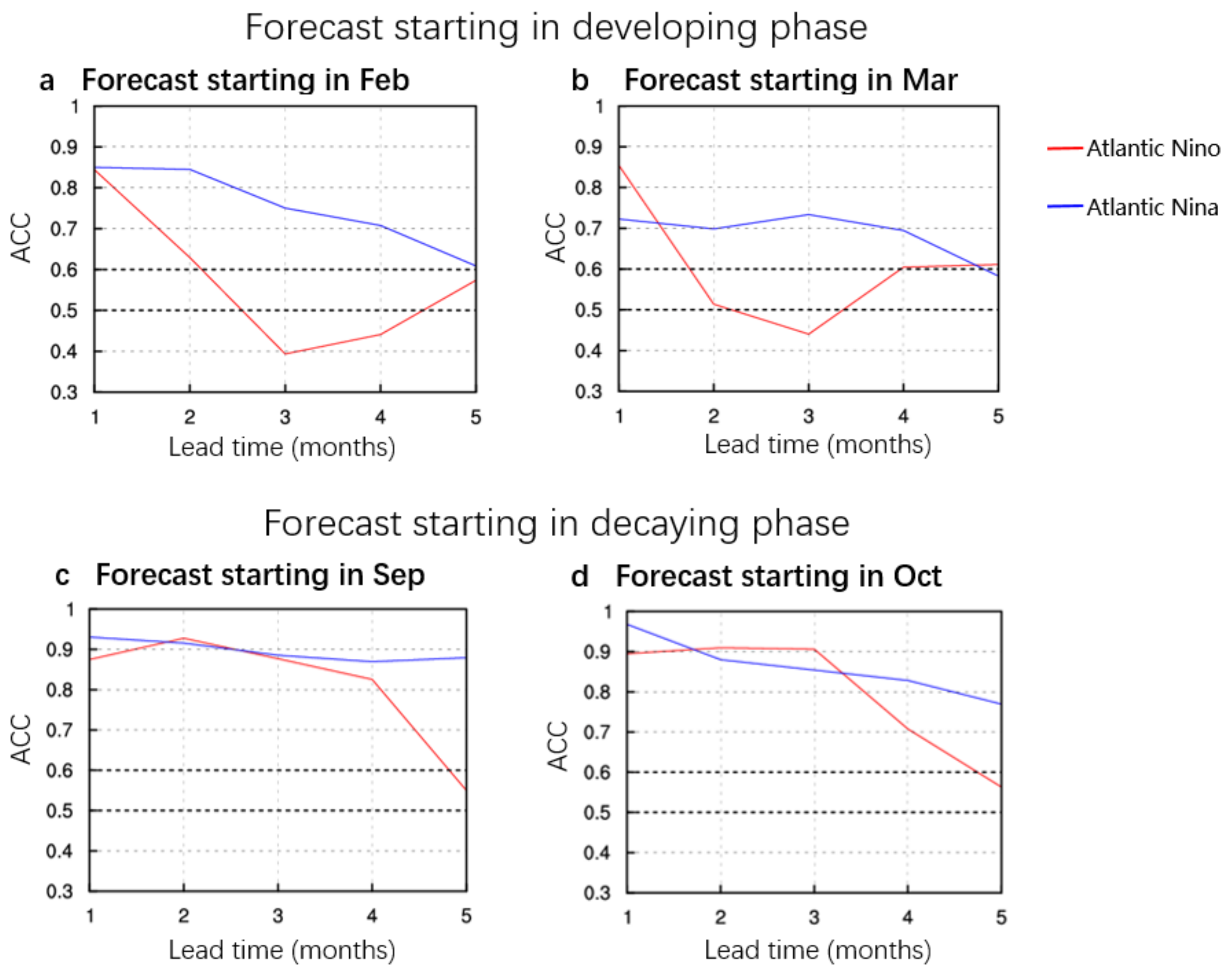
- The more detailed assessments document that the prediction skill for Atlantic Niña is higher than that for Atlantic Niño, and the prediction skill in the developing phase is better than that in the decaying phase. A preliminary analysis reveals that all the models show that the SNR for the Atlantic Niña prediction is obviously larger than the SNR for the Atlantic Niño prediction, indicating that the Atlantic Niña is more predictable than Atlantic Niño. The contrasting potential predictability estimated by SNR may partly explain why the prediction skill of Atlantic Niña is higher than that of Atlantic Niño in NMME models.
- (5)
- Our further analysis show that the amplitude bias of the predicted Atlantic Niño/Niña is primarily attributed to the amplitude bias of the annual cycle of SST, while the mean state bias (e.g., mean SST bias in Atl3 region) and the amplitude bias of Niño3.4 index are not the common factors among the models. Generally speaking, a weak annual cycle of SST corresponds to an underestimation of the Atlantic Niño/Niña variability, and vice versa. The detailed reason behind this needs further investigation in the future. From the perspective of ACC scores, we found that the prediction skill for the Atlantic Niño/Niña events, to a large extent, relies on the prediction skill for the preceding boreal winter (December–February) averaged Niño3.4 index (or the preceding ENSO).
Author Contributions
Funding
Institutional Review Board Statement
Informed Consent Statement
Data Availability Statement
Acknowledgments
Conflicts of Interest
References
- Li, X.; Xie, S.-P.; Gille, S.T.; Yoo, C. Atlantic-induced pan-tropical climate change over the past three decades. Nat. Clim. Chang. 2016, 6, 275–279. [Google Scholar] [CrossRef]
- Jin, E.K.; Kinter, J.L.; Wang, B.; Park, C.-K.; Kang, I.-S.; Kirtman, B.P.; Kug, J.-S.; Kumar, A.; Luo, J.-J.; Schemm, J.; et al. Current status of ENSO prediction skill in coupled ocean—Atmosphere models. Clim. Dyn. 2008, 31, 647–664. [Google Scholar] [CrossRef]
- Wang, C.; Kucharski, F.; Barimalala, R.; Bracco, A. Teleconnections of the tropical Atlantic to the tropical Indian and Pacific Oceans: A review of recent findings. Meteorol. Z. 2009, 18, 445–454. [Google Scholar] [CrossRef]
- Lübbecke, J.F.; Rodríguez-Fonseca, B.; Richter, I.; Martín-Rey, M.; Losada, T.; Polo, I.; Keenlyside, N.S. Equatorial Atlantic variability—Modes, mechanisms, and global teleconnections. Wiley Interdiscip. Rev. Clim. Chang. 2018, 9, e527. [Google Scholar] [CrossRef]
- Tang, Y.; Zhang, R.-H.; Liu, T.; Duan, W.; Yang, D.; Zheng, F.; Ren, H.; Lian, T.; Gao, C.; Chen, D.; et al. Progress in ENSO prediction and predictability study. Natl. Sci. Rev. 2018, 5, 826–839. [Google Scholar] [CrossRef]
- Nobre, P.; Shukla, J. Variations of Sea Surface Temperature, Wind Stress, and Rainfall over the Tropical Atlantic and South America. J. Clim. 1996, 9, 2464–2479. [Google Scholar] [CrossRef]
- Folland, C.K.; Colman, A.W.; Rowell, D.P.; Davey, M.K. Predictability of Northeast Brazil Rainfall and Real-Time Forecast Skill, 1987–98. J. Clim. 2001, 14, 1937–1958. [Google Scholar] [CrossRef]
- Giannini, A.; Saravanan, R.; Chang, P. The preconditioning role of Tropical Atlantic Variability in the development of the ENSO teleconnection: Implications for the prediction of Nordeste rainfall. Clim. Dyn. 2004, 22, 839–855. [Google Scholar] [CrossRef]
- Wang, C. Three-ocean interactions and climate variability: A review and perspective. Clim. Dyn. 2019, 53, 5119–5136. [Google Scholar] [CrossRef]
- Zebiak, S.E. Air–Sea Interaction in the Equatorial Atlantic Region. J. Clim. 1993, 6, 1567–1586. [Google Scholar] [CrossRef]
- Murtugudde, R.G.; Beauchamp, J.; Busalacchi, A.J.; Ballabrera-Poy, J. Relationship between zonal and meridional modes in the tropical Atlantic. Geophys. Res. Lett. 2001, 28, 4463–4466. [Google Scholar] [CrossRef]
- Polo, I.; Rodríguez-Fonseca, B.; Losada, T.; García-Serrano, J. Tropical Atlantic Variability Modes (1979–2002). Part I: Time-Evolving SST Modes Related to West African Rainfall. J. Clim. 2008, 21, 6457–6475. [Google Scholar] [CrossRef]
- Xie, S.-P.; Carton, J.A.; Wang, C. Tropical Atlantic Variability: Patterns, Mechanisms, and Impacts. Large Igneous Prov. 2013, 147, 121–142. [Google Scholar] [CrossRef]
- Chang, P.; Fang, Y.; Saravanan, R.; Ji, L.; Seidel, H. The cause of the fragile relationship between the Pacific El Niño and the Atlantic Niño. Nature 2006, 443, 324–328. [Google Scholar] [CrossRef]
- Keenlyside, N.S.; Latif, M. Understanding Equatorial Atlantic Interannual Variability. J. Clim. 2007, 20, 131–142. [Google Scholar] [CrossRef]
- Lübbecke, J.F.; McPhaden, M.J. On the Inconsistent Relationship between Pacific and Atlantic Niños. J. Clim. 2012, 25, 4294–4303. [Google Scholar] [CrossRef]
- Richter, I.; Xie, S.-P.; Morioka, Y.; Doi, T.; Taguchi, B.; Behera, S. Phase locking of equatorial Atlantic variability through the seasonal migration of the ITCZ. Clim. Dyn. 2017, 48, 3615–3629. [Google Scholar] [CrossRef]
- Carton, J.A.; Huang, B. Warm Events in the Tropical Atlantic. J. Phys. Oceanogr. 1994, 24, 888–903. [Google Scholar] [CrossRef]
- Wang, B.; Xiang, B.; Lee, J.-Y. Subtropical High predictability establishes a promising way for monsoon and tropical storm predictions. Proc. Natl. Acad. Sci. USA 2013, 110, 2718–2722. [Google Scholar] [CrossRef] [PubMed]
- Luo, J.-J.; Masson, S.; Behera, S.K.; Yamagata, T. Extended ENSO Predictions Using a Fully Coupled Ocean–Atmosphere Model. J. Clim. 2008, 21, 84–93. [Google Scholar] [CrossRef]
- Wang, B.; Lee, J.-J.; Kang, I.-S.; Shukla, J.; Park, C.-K.; Kumar, A.; Schemm, J.; Cocke, S.; Kug, J.-S.; Luo, J.-J.; et al. Advance and prospectus of seasonal prediction: Assessment of the APCC/ CliPAS 14-model ensemble retrospective seasonal prediction (1980–2004). Clim. Dyn. 2009, 33, 93–117. [Google Scholar] [CrossRef]
- Kumar, A.; Hu, Z.-Z.; Jha, B.; Peng, P. Estimating ENSO predictability based on multi-model hindcasts. Clim. Dyn. 2017, 48, 39–51. [Google Scholar] [CrossRef]
- Zheng, F.; Zhu, J.; Wang, H.; Zhang, R.-H. Ensemble hindcasts of ENSO events over the past 120 years using a large number of ensembles. Adv. Atmospheric Sci. 2009, 26, 359–372. [Google Scholar] [CrossRef]
- Zheng, F.; Zhu, J. Improved ensemble-mean forecasting of ENSO events by a zero-mean stochastic error model of an intermediate coupled model. Clim. Dyn. 2016, 47, 3901–3915. [Google Scholar] [CrossRef]
- Zhang, R.-H.; Yu, Y.; Song, Z.; Ren, H.-L.; Tang, Y.; Qiao, F.; Wu, T.; Gao, C.; Hu, J.; Tian, F.; et al. A review of progress in coupled ocean-atmosphere model developments for ENSO studies in China. J. Oceanol. Limnol. 2020, 38, 930–961. [Google Scholar] [CrossRef]
- Zhang, R.-H.; Gao, C. The IOCAS intermediate coupled model (IOCAS ICM) and its real-time predictions of the 2015–2016 El Niño event. Sci. Bull. 2016, 61, 1061–1070. [Google Scholar] [CrossRef]
- Luo, J.-J.; Masson, S.; Behera, S.; Yamagata, T. Experimental Forecasts of the Indian Ocean Dipole Using a Coupled OAGCM. J. Clim. 2007, 20, 2178–2190. [Google Scholar] [CrossRef]
- Liu, H.; Tang, Y.; Chen, D.; Lian, T. Predictability of the Indian Ocean Dipole in the coupled models. Clim. Dyn. 2016, 48, 2005–2024. [Google Scholar] [CrossRef]
- Tan, X.; Tang, Y.; Lian, T.; Zhang, S.; Liu, T.; Chen, D. Effects of Semistochastic Westerly Wind Bursts on ENSO Predictability. Geophys. Res. Lett. 2020, 47, 086828. [Google Scholar] [CrossRef]
- Doi, T.; Storto, A.; Behera, S.K.; Navarra, A.; Yamagata, T. Improved Prediction of the Indian Ocean Dipole Mode by Use of Subsurface Ocean Observations. J. Clim. 2017, 30, 7953–7970. [Google Scholar] [CrossRef]
- Wang, F.; Chang, P. A Linear Stability Analysis of Coupled Tropical Atlantic Variability. J. Clim. 2008, 21, 2421–2436. [Google Scholar] [CrossRef]
- Thompson, C.J.; Battisti, D.S. A Linear Stochastic Dynamical Model of ENSO. Part I: Model Development. J. Clim. 2000, 13, 2818–2832. [Google Scholar] [CrossRef]
- Thompson, C.J.; Battisti, D.S. A Linear Stochastic Dynamical Model of ENSO. Part II: Analysis. J. Clim. 2001, 14, 445–466. [Google Scholar] [CrossRef]
- Li, X.; Bordbar, M.H.; Latif, M.; Park, W.; Harlaß, J. Monthly to seasonal prediction of tropical Atlantic sea surface temperature with statistical models constructed from observations and data from the Kiel Climate Model. Clim. Dyn. 2020, 54, 1829–1850. [Google Scholar] [CrossRef]
- Stockdale, T.N.; Balmaseda, M.A.; Vidard, A. Tropical Atlantic SST Prediction with Coupled Ocean–Atmosphere GCMs. J. Clim. 2006, 19, 6047–6061. [Google Scholar] [CrossRef]
- Hu, Z.-Z.; Huang, B. The Predictive Skill and the Most Predictable Pattern in the Tropical Atlantic: The Effect of ENSO. Mon. Weather Rev. 2007, 135, 1786–1806. [Google Scholar] [CrossRef]
- Kirtman, B.P.; Min, D.; Infanti, J.M.; Kinter, J.L.; Paolino, D.A.; Zhang, Q.; Dool, H.V.D.; Saha, S.; Mendez, M.P.; Becker, E.; et al. The North American Multimodel Ensemble: Phase-1 Seasonal-to-Interannual Prediction; Phase-2 toward Developing Intraseasonal Prediction. Bull. Am. Meteorol. Soc. 2014, 95, 585–601. [Google Scholar] [CrossRef]
- Becker, E.; Dool, H.V.D.; Zhang, Q. Predictability and Forecast Skill in NMME. J. Clim. 2014, 27, 5891–5906. [Google Scholar] [CrossRef]
- Chen, L.C.; Huug, V.D.D.; Becker, E.; Zhang, Q. ENSO Precipitation and Temperature Forecasts in the North American Multi-Model Ensemble: Composite Analysis and Validation. Am. Meteorol. Soc. 2017, 30, 1103–1125. [Google Scholar]
- Zhang, W.; Villarini, G.; Slater, L.; Vecchi, G.; Bradley, A. Improved ENSO Forecasting Using Bayesian Updating and the North American Multimodel Ensemble (NMME). J. Clim. 2017, 30, 9007–9025. [Google Scholar] [CrossRef]
- Wu, Y.; Tang, Y. Seasonal predictability of the tropical Indian Ocean SST in the North American multimodel ensemble. Clim. Dyn. 2019, 53, 3361–3372. [Google Scholar] [CrossRef]
- Pillai, P.A.; Rao, S.A.; Ramu, D.A.; Pradhan, M.; George, G. Seasonal prediction skill of Indian summer monsoon rainfall in NMME models and monsoon mission CFSv2. Int. J. Clim. 2018, 38, e847–e861. [Google Scholar] [CrossRef]
- Singh, B.; Cash, B.; Iii, J.L.K. Indian summer monsoon variability forecasts in the North American multimodel ensemble. Clim. Dyn. 2019, 53, 7321–7334. [Google Scholar] [CrossRef]
- Hua, L.; Su, J. Southeastern Pacific error leads to failed El Niño forecasts. Geophys. Res. Lett. 2020, 47, 088764. [Google Scholar] [CrossRef]
- Newman, M.; Sardeshmukh, P.D. Are we near the predictability limit of tropical Indo-Pacific sea surface temperatures? Geophys. Res. Lett. 2017, 44, 8520–8529. [Google Scholar] [CrossRef]
- Lee, D.E.; Chapman, D.; Henderson, N.; Chen, C.; Cane, M.A. Multilevel vector autoregressive prediction of sea surface temperature in the North Tropical Atlantic Ocean and the Caribbean Sea. Clim. Dyn. 2016, 47, 95–106. [Google Scholar] [CrossRef]
- Harnos, D.S.; Schemm, J.-K.E.; Wang, H.; Finan, C.A. NMME-based hybrid prediction of Atlantic hurricane season activity. Clim. Dyn. 2017, 53, 7267–7285. [Google Scholar] [CrossRef]
- Richter, I.; Doi, T.; Behera, S.K.; Keenlyside, N. On the link between mean state biases and prediction skill in the tropics: An atmospheric perspective. Clim. Dyn. 2018, 50, 3355–3374. [Google Scholar] [CrossRef]
- Penland, C.; Matrosova, L. Prediction of Tropical Atlantic Sea Surface Temperatures Using Linear Inverse Modeling. J. Clim. 1998, 11, 483–496. [Google Scholar] [CrossRef]
- Xu, Z.; Chang, P.; Richter, I.; Kim, W.; Tang, G. Diagnosing southeast tropical Atlantic SST and ocean circulation biases in the CMIP5 ensemble. Clim. Dyn. 2014, 43, 3123–3145. [Google Scholar] [CrossRef]
- Richter, I.; Xie, S.-P.; Behera, S.K.; Doi, T.; Masumoto, Y. Equatorial Atlantic variability and its relation to mean state biases in CMIP5. Clim. Dyn. 2014, 42, 171–188. [Google Scholar] [CrossRef]
- Huang, B.; Schopf, P.S.; Shukla, J. Intrinsic Ocean–Atmosphere Variability of the Tropical Atlantic Ocean. J. Clim. 2004, 17, 2058–2077. [Google Scholar] [CrossRef]
- Exarchou, E.; Prodhomme, C.; Brodeau, L.; Guemas, V.; Doblas-Reyes, F. Origin of the warm eastern tropical Atlantic SST bias in a climate model. Clim. Dyn. 2017, 51, 1819–1840. [Google Scholar] [CrossRef]
- Vallès-Casanova, I.; Lee, S.; Foltz, G.R.; Pelegrí, J.L. On the Spatiotemporal Diversity of Atlantic Niño and Associated Rainfall Variability Over West Africa and South America. Geophys. Res. Lett. 2020, 47, 087108. [Google Scholar] [CrossRef]
- Rayner, N.A.; Parker, D.E.; Horton, E.B.; Folland, C.K.; Alexander, L.V.; Rowell, D.P.; Kent, E.; Kaplan, A.L. Global analyses of sea surface temperature, sea ice, and night marine air temperature since the late nineteenth century. J. Geophys. Res. Space Phys. 2003, 108, 108. [Google Scholar] [CrossRef]
- Luo, J.-J.; Behera, S.K.; Masumoto, Y.; Yamagata, T. Impact of Global Ocean Surface Warming on Seasonal-to-Interannual Climate Prediction. J. Clim. 2011, 24, 1626–1646. [Google Scholar] [CrossRef]
- Kirtman, B.P.; Huang, B.; Zhu, Z.; Schneider, E.K. Multi-seasonal prediction with a coupled tropical ocean—Global at-mosphere system. Am. Meteorol. Soc. 1997, 125, 789–808. [Google Scholar]
- Ham, Y.-G.; Kim, J.-H.; Luo, J.-J. Deep learning for multi-year ENSO forecasts. Nat. Cell Biol. 2019, 573, 568–572. [Google Scholar] [CrossRef]
- Luo, J.-J.; Masson, S.; Behera, S.K.; Shingu, S.; Yamagata, T. Seasonal Climate Predictability in a Coupled OAGCM Using a Different Approach for Ensemble Forecasts. J. Clim. 2005, 18, 4474–4497. [Google Scholar] [CrossRef]
- Zhao, S.; Stuecker, M.F.; Jin, F.-F.; Feng, J.; Ren, H.-L.; Zhang, W.; Li, J. Improved Predictability of the Indian Ocean Dipole Using a Stochastic Dynamical Model Compared to the North American Multimodel Ensemble Forecast. Weather Forecast. 2020, 35, 379–399. [Google Scholar] [CrossRef]
- Latif, M.; Barnett, T.P.; Cane, M.A.; Flügel, M.; Graham, N.E.; von Storch, H.; Xu, J.-S.; Zebiak, S.E. A review of ENSO prediction studies. Clim. Dyn. 1994, 9, 167–179. [Google Scholar] [CrossRef]
- Webster, P.J.M. The annual cycle and the predictability of the tropical coupled ocean-atmosphere system. Meteorol. Atmos. Phys. 1995, 56, 33–55. [Google Scholar] [CrossRef]
- Lopez, H.; Kirtman, B.P. WWBs, ENSO predictability, the spring barrier and extreme events. J. Geophys. Res. Atmos. 2014, 119, 10–114. [Google Scholar] [CrossRef]
- Larson, S.M.; Pegion, K. Do asymmetries in ENSO predictability arise from different recharged states? Clim. Dyn. 2019, 54, 1507–1522. [Google Scholar] [CrossRef]
- Hu, Z.-Z.; Kumar, A.; Zhu, J. Dominant modes of ensemble mean signal and noise in seasonal forecasts of SST. Clim. Dyn. 2021, 56, 1251–1264. [Google Scholar] [CrossRef]
- Tippett, M.K.; Ranganathan, M.; L’Heureux, M.; Barnston, A.G.; Delsole, T. Assessing probabilistic predictions of ENSO phase and intensity from the North American Multimodel Ensemble. Clim. Dyn. 2017, 53, 7497–7518. [Google Scholar] [CrossRef]
- Kirtman, B.P. The COLA Anomaly Coupled Model: Ensemble ENSO Prediction. Mon. Weather Rev. 2003, 131, 2324–2341. [Google Scholar] [CrossRef]
- Liu, T.; Tang, Y.; Yang, D.; Cheng, Y.; Song, X.; Hou, Z.; Shen, Z.; Gao, Y.; Wu, Y.; Li, X.; et al. The relationship among probabilistic, deterministic and potential skills in predicting the ENSO for the past 161 years. Clim. Dyn. 2019, 53, 6947–6960. [Google Scholar] [CrossRef]
- Li, T.; Philander, S.G.H. On the Seasonal Cycle of the Equatorial Atlantic Ocean. J. Clim. 1997, 10, 813–817. [Google Scholar] [CrossRef][Green Version]
- Ding, H.; Keenlyside, N.; Latif, M.; Park, W.; Wahl, S. The impact of mean state errors on equatorial A tlantic interannual variability in a climate model. J. Geophys. Res. Oceans 2015, 120, 1133–1151. [Google Scholar] [CrossRef]
- Lee, J.-Y.; Wang, B.; Kang, I.-S.; Shukla, J.; Kumar, A.; Kug, J.-S.; Schemm, J.K.E.; Luo, J.-J.; Yamagata, T.; Fu, X.; et al. How are seasonal prediction skills related to models’ performance on mean state and annual cycle? Clim. Dyn. 2010, 35, 267–283. [Google Scholar] [CrossRef]
- Cai, W.; Wu, L.; Lengaigne, M.; Li, T.; McGregor, S.; Kug, J.-S.; Yu, J.-Y.; Stuecker, M.F.; Santoso, A.; Li, X.; et al. Pantropical climate interactions. Science 2019, 363, eaav4236. [Google Scholar] [CrossRef]
- Wang, C. ENSO, Atlantic Climate Variability, and the Walker and Hadley Circulations. In The Hadley Circulation: Present, Past and Future; Springer: Dordrecht, The Netherlands, 2004; Volume 21, pp. 173–202. [Google Scholar]
- Wang, C. An overlooked feature of tropical climate: Inter-Pacific-Atlantic variability. Geophys. Res. Lett. 2006, 33, 12702. [Google Scholar] [CrossRef]


| NMME Partner | Model Name | AGCM | OGCM | Max Lead (Months) | Ensemble Members | Hindcast Period | |
|---|---|---|---|---|---|---|---|
| NMME-Phase 1 | CanCM4i * | CanAM4 T63 L31 | CanOM4 L40 0.94° Eq | 12 | 10 | 1981–2010 | |
| CanSIPSv2 * | CanAM4 T63 L35 | CanOM4 1.4° × 0.94° L40 | 12 | 20 | 1981–2010 | ||
| CMC1-CanCM3 * | CanAM3 T63 L31 | CanOM4 L40 0.94° Eq | 12 | 10 | 1981–2010 | ||
| CMC2-CanCM4 * | CanAM4 T63 L35 | CanOM4 L40 0.94° Eq | 12 | 10 | 1981–2010 | ||
| GEM-NEMO * | GEM 256 × 128 (1.4°) | NEMO 1° × 1° 1/3° Eq | 12 | 10 | 1981–2010 | ||
| NASA-GEOSS2S | GEOS5 AGCM 0.5° L72 | MOM5 L40 0.5° Eq | 10 | 10 | 1981–2016 | ||
| NCAR-CESM1 | 0.9° × 1.25° L30 | POP L60 0.25° Eq | 12 | 10 | 1982–2010 | ||
| NCEP-CFSv2 | GFS T12 L64 | MOM4 L40 0.25° Eq | 10 | 24 | 1982–2010 | ||
| NMME-Phase 2 | CanCM3 * | CanAM3 T63 L31 | CanOM4 L40 | 12 | 10 | 1981–2011 | |
| CanCM4 * | CanAM4 T63 L35 | CanOM4 L40 | 12 | 10 | 1981–2011 | ||
| CCSM4 | 1.25° × 0.9° L26 | L60 1.13° × 0.27° Eq | 12 | 10 | 1982–2010 | ||
| CESM1 * | 1.25° × 0.9° L30 | L60 1.13° × 0.27° Eq | 12 | 10 | 1980–2010 | ||
| FLORB-01 | CM2.5 0.5° L32 | CM2.1 1° × 1°, 0.333° Eq | 12 | 10 | 1980–2013 | ||
| STD of Atl3 Index | |
|---|---|
| Observation (198201–201012) | 0.465 |
| Two-month-lead MME (198202–201101) | 0.296 |
| Three-month-lead MME (198203–201102) | 0.245 |
| Four-month-lead MME (198204–201103) | 0.213 |
| Five-month-lead MME (198205–201104) | 0.192 |
Publisher’s Note: MDPI stays neutral with regard to jurisdictional claims in published maps and institutional affiliations. |
© 2021 by the authors. Licensee MDPI, Basel, Switzerland. This article is an open access article distributed under the terms and conditions of the Creative Commons Attribution (CC BY) license (https://creativecommons.org/licenses/by/4.0/).
Share and Cite
Wang, R.; Chen, L.; Li, T.; Luo, J.-J. Atlantic Niño/Niña Prediction Skills in NMME Models. Atmosphere 2021, 12, 803. https://doi.org/10.3390/atmos12070803
Wang R, Chen L, Li T, Luo J-J. Atlantic Niño/Niña Prediction Skills in NMME Models. Atmosphere. 2021; 12(7):803. https://doi.org/10.3390/atmos12070803
Chicago/Turabian StyleWang, Ran, Lin Chen, Tim Li, and Jing-Jia Luo. 2021. "Atlantic Niño/Niña Prediction Skills in NMME Models" Atmosphere 12, no. 7: 803. https://doi.org/10.3390/atmos12070803
APA StyleWang, R., Chen, L., Li, T., & Luo, J.-J. (2021). Atlantic Niño/Niña Prediction Skills in NMME Models. Atmosphere, 12(7), 803. https://doi.org/10.3390/atmos12070803