Article

Assessment of the Urban Impact on Surface and Screen-Level Temperature in the ALADIN-Climate Driven SURFEX Land Surface Model for Budapest

by
Gabriella Zsebeházi
1,* and
Sándor István Mahó
2
1
Hungarian Meteorological Service, 1024 Budapest, Hungary
2
Department of Physics, University of Helsinki, 00014 Helsinki, Finnland
*
Author to whom correspondence should be addressed.
Atmosphere 2021, 12(6), 709; https://doi.org/10.3390/atmos12060709
Submission received: 31 March 2021 / Revised: 10 May 2021 / Accepted: 28 May 2021 / Published: 31 May 2021

Abstract

:
Land surface models with detailed urban parameterization schemes provide adequate tools to estimate the impact of climate change in cities, because they rely on the results of the regional climate model, while operating on km scale at low cost. In this paper, the SURFEX land surface model driven by the evaluation and control runs of ALADIN-Climate regional climate model is validated over Budapest from the aspect of urban impact on temperature. First, surface temperature of SURFEX with forcings from ERA-Interim driven ALADIN-Climate was compared against the MODIS land surface temperature for a 3-year period. Second, the impact of the ARPEGE global climate model driven ALADIN-Climate was assessed on the 2 m temperature of SURFEX and was validated against measurements of a suburban station for 30 years. The spatial extent of surface urban heat island (SUHI) is exaggerated in SURFEX from spring to autumn, because the urbanized gridcells are generally warmer than their rural vicinity, while the observed SUHI extent is more variable. The model reasonably simulates the seasonal means and diurnal cycle of the 2 m temperature in the suburban gridpoint, except summer when strong positive bias occurs. However, comparing the two experiments from the aspect of nocturnal UHI, only minor differences arose. The thorough validation underpins the applicability of SURFEX driven by ALADIN-Climate for future urban climate projections.

1. Introduction

Urbanized surfaces are characterized by highly different surface properties (e.g., imperviousness, large roughness, large heat capacity, and heat admittance of materials) from natural surfaces, that leads to altered energy budget components and boundary layer properties. One of the most studied and well-known manifestations of these differences is the higher surface, subsurface and air temperature in the city, forming the urban heat island (UHI) [1]. More than half of the world’s population lives now in urban settlements, although the impervious surfaces occupy less than 0.5% of the Earth [2]. Such high population density can be observed in Hungary as well; for example, the Budapest urban agglomeration occupies 2.7% of the territory of Hungary, while its 2.5 million inhabitants represent one quarter of the whole country’s population [3]. As a consequence of the high population density and elevated temperatures, cities are exposed to more severe heat related risks compared to rural areas. With climate change, this exposure may be further exacerbated, negatively affecting for example human health, environment and energy demand [4].
By the increasing resolution and complexity of global and regional climate models (GCMs and RCMs), urban processes tend to be parameterized, giving a first approximation about the impact of climate change on cities [5]. For example, it was shown that global climate models with urban parameterization schemes portray urban heat island and altered surface fluxes over the cities [6,7]. In [8,9] a slab model (i.e., cities are represented by rocks) and the town energy balance (TEB) urban canopy model implemented in the climate version of the Aire Limitée Adaptation dynamique Dévéloppement INternational (ALADIN-Climate) RCM and the ALadin-AROme (ALARO, where AROME stands for Application of Research to Operations at MEsoscale) limited area numerical weather prediction model, respectively, were compared and found that the more complex parameterization improves the UHI representation. A subset of the Euro-CORDEX (the European branch of the COordinated Regional Downscaling EXperiment) 0.11° resolution regional climate models (which approximate urban processes with bulk formulas) were evaluated from the aspect of temperature and humidity over Berlin and demonstrated that the models are capable of resulting in substantially drier and warmer conditions over the city compared to rural areas [10]. Despite the positive impact of urban parameterization in global and regional climate models, these models cannot necessarily resolve the intra-urban and subdaily features of urban climate (e.g., daily humidity cycle) due to their relatively coarse resolution and in some cases due to the simple bulk formulas [10].
In contrast, convection permitting climate models resolve urban climate processes on km scale and show added value on simulating cities’ feedback to the atmosphere. For example, the UHI impact on precipitation using the Weather Research Forecast (WRF) model was investigated over northern Taiwan [11]. The drawback of such fine scale models is that they require vast computer capacity. Therefore, to date it is hardly possible to apply them on transient mode or downscale a large number of GCMs.
The offline land surface models (LSMs) that comprise detailed urban parameterization scheme [12,13,14] provide adequate tools to eliminate the abovementioned drawbacks. These models are directly forced by the RCM outputs, therefore they can simulate the long-term impact of climate change on cities at high resolution (a couple of hundred meters to a couple of km) but at low cost. In this paper, the SURFace EXternalisée (SURFEX) land surface model that uses the TEB scheme over urbanized surfaces is evaluated for temperature and UHI, following the classical validation process applied in regional climate modelling. For this reason, SURFEX is forced by an evaluation and a control experiment of an RCM (in which case the RCM is driven by a reanalysis and a GCM, respectively).
The traditional method for climate model validation is to compare the simulation results with gridded dataset constructed from in situ observations [15]. Nevertheless, this approach is not representative enough for urban areas, since the resolution of the available gridded observational datasets are generally not more than 10 km (e.g., E-OBS [16]; CarpatClim-Hu [17]). Therefore, a very dense station network would be needed for the validation, which can represent different built-up classes within a city and the spatial characteristics of urban climate [18,19]. This need has been recognized and a number of measurement initiatives have been started in recent years [20,21,22]. In Hungary such an observation network has been operating since 2014 in Szeged, although its measurement period does not intersect with the common evaluation period of climate models that ends before 2005. Therefore, two alternatives can be used to evaluate fine scale urban simulations. (1) Satellite land surface temperature (LST) products have become widely available since the 2000s having appropriate spatial resolution for reflecting urban atmospheric characteristics [23] and global coverage [24]. (2) A few station measurements from the city and from the suburban region are available for assessment the temporal characteristics of the urban impact in the LSM on climate timescale [25].
The aim of the present study is to evaluate the SURFEX LSM over Budapest and its rural surrounding. SURFEX is driven by the ALADIN-Climate RCM that was driven by the ERA-Interim and the Action de Recherche Petite Echelle Grande Echelle (ARPEGE), that is the atmospheric component of the Centre National de Recherches Météorologiques Coupled global climate Model (CNRM-CM) GCM. The focus of this paper is to scrutinize SURFEX from the aspect of urban surface impact on 2 m and surface temperature, and the spatial and temporal characteristics of urban climate. Therefore, the model simulations are validated against Moderate Resolution Imaging Spectroradiometer Sensor (MODIS) LST data on a 3 year period and against the synoptic station measurement on a 30 year period. Section 2 presents the SURFEX model, the evaluation and control simulation of the ALADIN-Climate providing forcings for SURFEX, the considered observations and the evaluation methods and measures. Section 3 is dedicated to presenting the spatial characteristics of LST and surface UHI (SUHI), and the temporal characteristics of urban climate in one suburban gridpoint. The results are discussed in Section 4 and finally, Section 5 summarizes our conclusions and presents future perspectives of our research.

2. Data and Methods

2.1. The SURFEX Land Surface Model

SURFEX [26] describes land surface processes in the lower 10% (a few 10 m) of the planetary boundary layer, called surface layer. The surface heterogeneity is handled by the tiling method, i.e., in each grid cell, the fractions of sea, inland water, town and natural land surface are given, and for each surface type (i.e., tile) a dedicated scheme computes the prognostic variables and turbulent fluxes. The total flux of the grid box is resulted by addition of the individual fluxes over the composing tiles. The land cover information is provided for the model by the first version of the ECOCLIMAP database [27]. From urban climate perspective, the continental cities and their vicinity can be described dominantly by the town and natural land surface types, therefore the schemes applied for them are presented hereinafter.
Over natural land surfaces the 3-layer Interaction Soil Biosphere Atmosphere scheme (ISBA-3L) [28] is used, that computes the surface and soil temperature and moisture with the force-restore method. This scheme divides the soil into three layers (a thin layer representing the surface, and two thicker layers for middle and deep soil), and the prognostic evolution of the temperature and moisture is described with a relatively simple formula.
The urban physical properties are calculated with the TEB scheme [29] that approximates the complexity of urban morphology with street canyons. Prognostic equations for the roof, wall and road specify the surface temperature and (except for wall) water content. The surfaces are divided into three layers in order to consider heat conductivity. Only domestic heating was considered as the source of anthropogenic heat flux by preventing the indoor temperature to fall below 19 °C. Note that in SURFEX there is a simple building energy model that can simulate the interaction of internal building temperature and the outdoor temperature. The near surface variables (e.g., 2 m temperature, humidity, 10 m wind speed) are calculated with the surface boundary layer (SBL) scheme [30,31] that divides the surface layer into six sub-layers and prognostically computes the temperature, humidity, wind and turbulence, taking into account the canopy and canyon effect and drag forces.

2.2. The Driving ALADIN-Climate Model

The atmospheric forcings of SURFEX are temperature, humidity, wind speed and wind direction at a few 10 m above ground level, downward shortwave and longwave radiation, surface pressure, snow and rain. In our case the forcings are provided by the ALADIN-Climate version 5.2 [32] hydrostatic spectral RCM. The physical parameterization package of ALADIN-Climate is derived from the ARPEGE-Climat version 5 [33] atmospheric GCM. The longwave radiation transfer is described by the Rapid Radiation Transfer Model (RRTM) scheme [34], while the shortwave radiation transfer is parameterized according to Fouquart and Bonnel [35]. The large-scale precipitation is determined by the Smith scheme [36], and the convective cloud and precipitation formation are described according to Bougeault [37]. The surface scheme of ALADIN is SURFEX version 5, in which ISBA-3L was applied over natural land surfaces. The vertical profile of temperature, humidity and windspeed in the surface layer is parameterized according to Geleyn [38]. Urbanized areas are substituted with rocks and the physical processes are described by the ISBA scheme.

2.3. Experimental Design

In this study, two urban climate simulations are performed with the 5.1 version of SURFEX for Budapest driven by the evaluation and control run of ALADIN-Climate 5.2 RCM. The ALADIN-Climate simulations were achieved at 10 km horizontal resolution on a domain covering Central and South-Eastern Europe (Figure 1). First, a 10-year long simulation was performed for 1996–2005 with SURFEX, where the lateral boundary conditions for ALADIN-Climate were derived from ERA-Interim [39]. This experiment allows to examine the RCM model’s influences on the behavior of SURFEX (hereinafter the RCM and LSM simulations are referred to ALADIN-EI and SURFEX-EI, respectively). Then, SURFEX was driven by the control simulation of ALADIN-Climate for 1960–2005 to evaluate SURFEX from a climate perspective. In this case, the lateral boundary conditions of ALADIN-Climate were the CNRM-CM5 GCM (hereinafter the RCM and LSM simulations are referred to ALADIN-ARP and SURFEX-ARP, respectively).
The SURFEX domain covers Budapest and its vicinity (Figure 1). It consists of 61 × 61 gridpoints with 1 km horizontal resolution. The main urban cover types over the domain are dense urban, temperate suburban, industrial and commercial areas, mineral extractions and construction sites, sport facilities, urban parks and airport according to ECOCLIMAP. The dominant natural cover types are Central European crops and temperate woodlands. 3 hourly outputs of ALADIN-Climate simulations derived at 30 m above ground level are considered as forcings. The ALADIN simulations are interpolated from 10 km to 1 km resolution using the 927 configuration of ALADIN-Climate (in general this configuration is used to prepare lateral boundary conditions for the RCM). The advantage of this method–in contrast to simply multiplying the gridpoints in each 10 km × 10 km gridcell–is that it takes into account the orography effect during interpolation, and it is crucial for a hilly domain. The integration timestep of SURFEX is 300 s, to which the 3 h forcings are linearly interpolated.

2.4. Observations

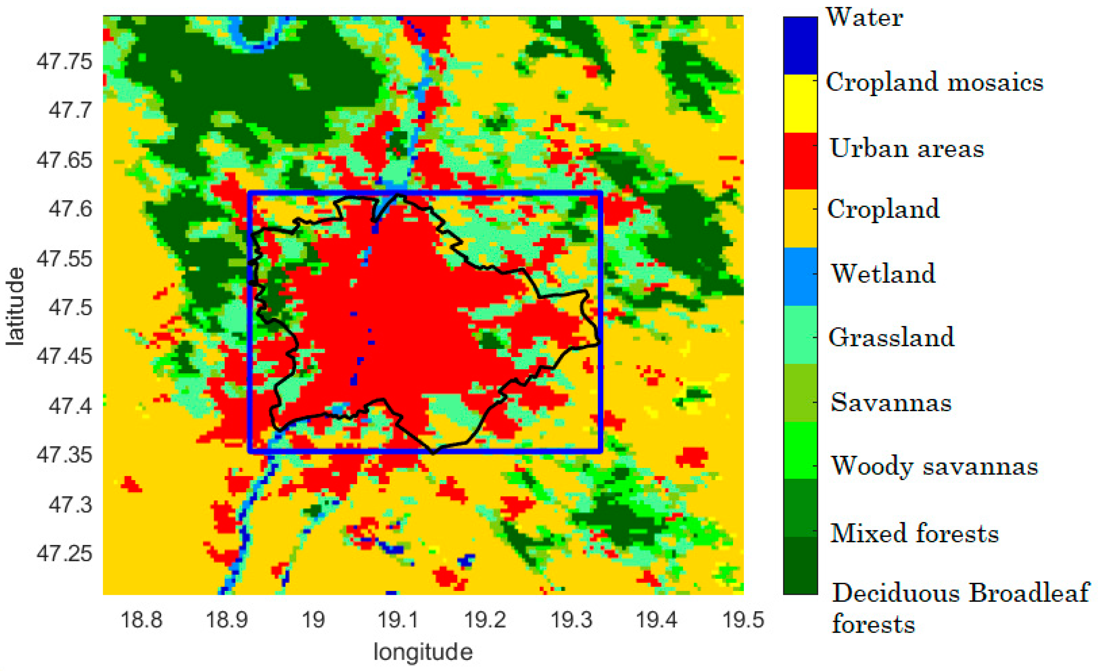
2.4.1. MODIS LST Product

Simulated surface temperature and SUHI over Budapest is studied against the MODIS Terra (from 1999) and Aqua (from 2000) LST product (version 6 of MOD11A1 and MYD11A1, respectively) [40,41]. The two polar orbit satellites acquire data in 36 spectral bands from 0.4 to 14.4 μm wavelengths [42]. The LST products are produced by the split-window method based on 7 spectral bands 4 times a day [43]. Table 1 shows the averaged satellite overpass time in UTC for Aqua and Terra over Budapest. The spatial resolution of the retrieved LST images are 1 km [19], which coincides with the spatial resolution of SURFEX LST fields.
The satellite observation data was first cleaned from the cloud contaminated grid cells in the following way: those times were excluded where the cloudy cells coverage exceeded 25 per cent of the whole domain. This filtering was applied for the SURFEX data as well using the mean total cloud cover of ALADIN-EI over Budapest, in order to keep the cloud-free cases only.
Finally, we applied the MODIS Terra + Aqua Combined Land Cover product [44,45] that includes the IGBP (International Geosphere-Biosphere Programme) land-use classification system which enabled us to select urban and non-urban grid cells in the MODIS LST analysis.

2.4.2. Gridded Observational Dataset and Station Measurements of 2 m Temperature

The 2 m temperature of SURFEX and ALADIN is evaluated against gridded and synoptic station measurements. The CarpatClim-Hu [17] gridded observation dataset was constructed based on homogenized and interpolated station measurements, and widely used for regional climate model evaluation for Hungary. Note that due to its 10 km resolution and the missing urban stations, urbanized areas are not emerging with higher temperatures in this dataset.
One station was chosen for pointwise validation based on the criteria of being continuously operated since 1970 and located in urbanized area. This station is situated in the Southeastern agglomeration area of Budapest (in Pestszentlőrinc) at 19°10′56″ E, 47°25′45″ N and at 139 m above sea level. The vicinity of the synoptic station is covered by grass, but the observatory is surrounded by houses with gardens except from south that is covered by forest (Figure 1). According to ECOCLIMAP, the closest gridpoint to the station is classified as temperate suburban, which consists of 60% urban area and 40% natural area.
In order to eliminate temporal inhomogeneities (originated from e.g., station relocation or change of instruments or measurement methods), the daily observation data was homogenized with the Multiple Analysis of Series for Homogenization (MASH) method [46].

2.5. Evaluation Methods

2.5.1. Surface Temperature and SUHI in SURFEX-EI

Since four measurements per day are available from the end of 2002 in MODIS (Table 2), we considered only the SURFEX-EI experiment on the period of 2003–2005 on a domain containing mainly urbanized and cropland areas (Figure 2).
SURFEX-ARP cannot be evaluated for such a short period, because it does not reflect the observed characteristics of the individual years (since it is driven by a GCM, in which only the observed greenhouse gas concentration describes the past reality, see Figure 8).
To compare the simulated value with the satellite data, the gridcell average surface temperature had to be computed beforehand, because it is not given by SURFEX v5. The mean surface temperature (LSTSURFEX) was derived based on the Stefan-Boltzmann law. Therefore, the emitted longwave radiations (LW) given by the TEB and ISBA schemes were taken (roof, wall and road values were averaged in TEB) using the same emissivity values (ε) as the model. Emissivity is constant in time and identical (0.97) for all natural land cover types, and for roof, wall and road as well (0.90, 0.85 and 0.94, respectively). Radiative surface temperature was produced for TEB and ISBA separately and the results were linearly combined according to the fraction of urban and nature land cover (xurban and 1 − xurban, respectively; Equation (1):
L S T S U R F E X = x u r b a n L W T E B ¯ σ ε ¯ T E B 4 + ( 1 x u r b a n ) L W I S B A σ ε I S B A 4
First, SURFEX simulations at 0 and 12 UTC–representing nighttime and daytime cases–were considered and compared with measurements of the Aqua satellite. Note that the measurements happen 30 min earlier around noon and 43 min later at night. We analyzed the seasonal mean daytime and nighttime LST and its variability to investigate how SURFEX is able to describe the spatial and temporal distribution of surface temperature over the urban and rural areas.
Afterwards SUHI affected area was determined based on the method of Zhang and Whang [47], which statistically defines the size of the area, which significantly differs in temperature from its environment. Following the method, we calculated the spatial mean surface temperature ( T ¯   in   ° C ) and standard deviation across gridpoints (σ in °C) in each timestep. Then, LST (T) in each gridpoint and timestep was categorized based on Equation (2):
{ T T ¯ + σ ,         S U H I   a f f e c t e d   g r i d p o i n t T < T ¯ + σ ,                                     o m i t t e d   g r i d p o i n t
Therefore, we identified those gridpoints as affected by SUHI where the temperature was higher than T ¯ + σ . The sum of the gridpoints, which fulfill this criterium were taken and divided by the number of all gridpoints for each timestep. This gave the relative SUHI affected area. In this analysis we considered a smaller domain bounded by the administrative border of Budapest (blue rectangle on Figure 2), because otherwise the relative SUHI affected area values (i.e., the proportion of SUHI affected gridcells and the all gridpoints of the domain) would be too low. The observed and modelled daily values are compared on histograms.
Finally, the seasonal mean diurnal cycle of SUHI and its variability was studied. SURFEX results were compared to all four measurements of Aqua and Terra, and SUHI was computed in the following way: in every timestep and in every gridpoint the LST was subtracted from the mean rural temperature. The mean rural temperature was determined as the average temperature of pure rural grid cells according to ECOCLIMAP in SURFEX and IGBP in MODIS.

2.5.2. 2 m Temperature in SURFEX-ARP

Besides short-term validation focusing on the urban surface temperature, the ability of SURFEX to reproduce long-term climate characteristics is assessed based on the SURFEX-ARP experiment. First, the temperature bias of ALADIN, and the interaction between ALADIN and SURFEX is briefly validated on 10 km resolution considering CarpatClim-Hu as reference (Table 2). Moreover, the performance of SURFEX is studied in one gridpoint, closest to the synoptic meteorological station in Pestszentlőrinc (Table 2). Measurements of 3-hourly and daily mean temperature were used to validate SURFEX in the period of 1971–2000. Annual and seasonal yearly mean values, distribution of daily mean temperatures and the mean diurnal cycle of 3 h temperature were assessed.

2.5.3. UHI in SURFEX-EI and SURFEX-ARP

Finally, SURFEX-EI and SURFEX-ARP was jointly evaluated and compared against each other, considering spatial distribution and seasonal mean diurnal cycle of UHI, and seasonal mean diurnal cycle of surface energy fluxes on a common 10-year period (1996–2005). The UHI were computed following the same method as was presented for SUHI in Section 2.5.1.

3. Results

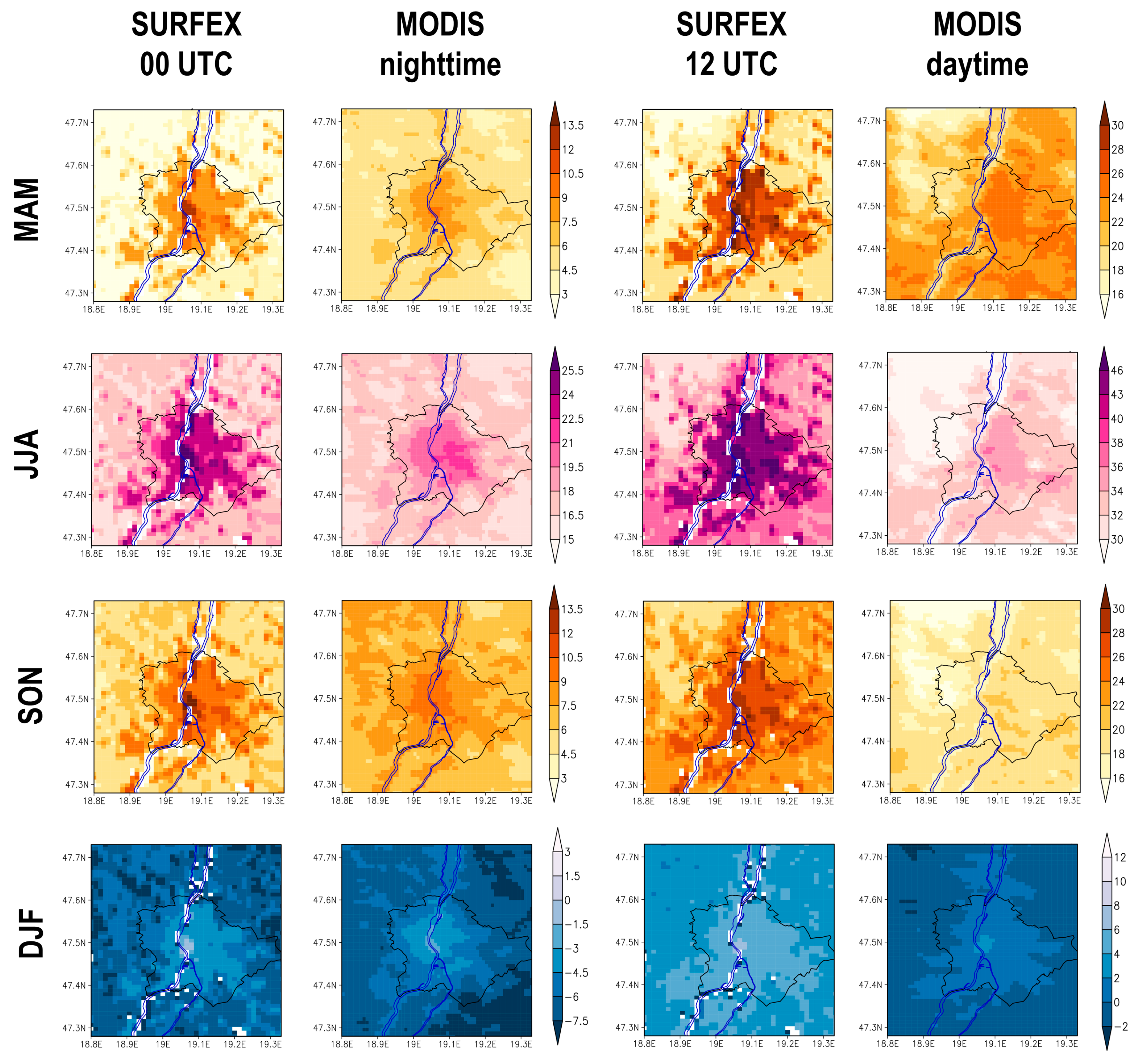
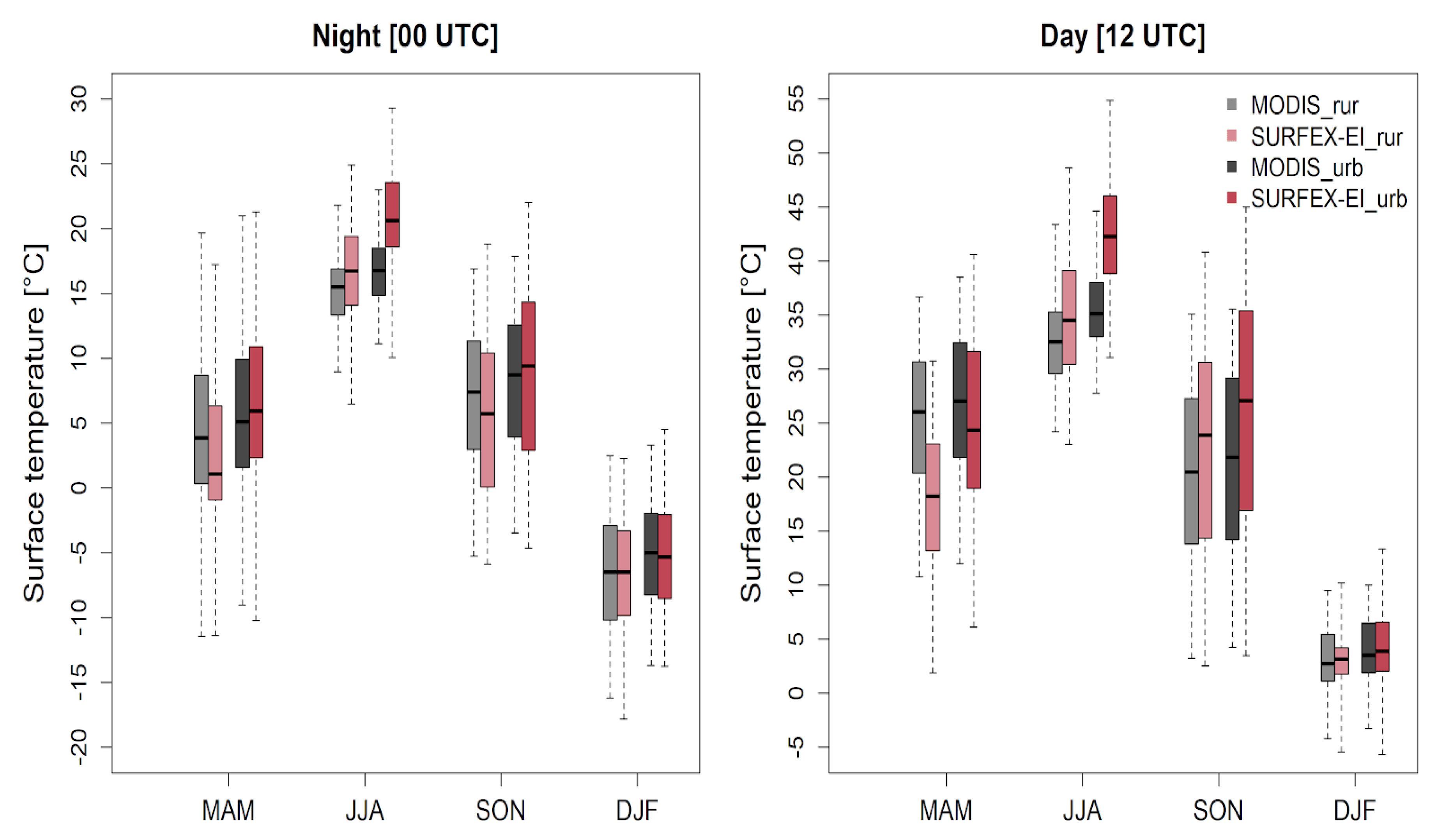
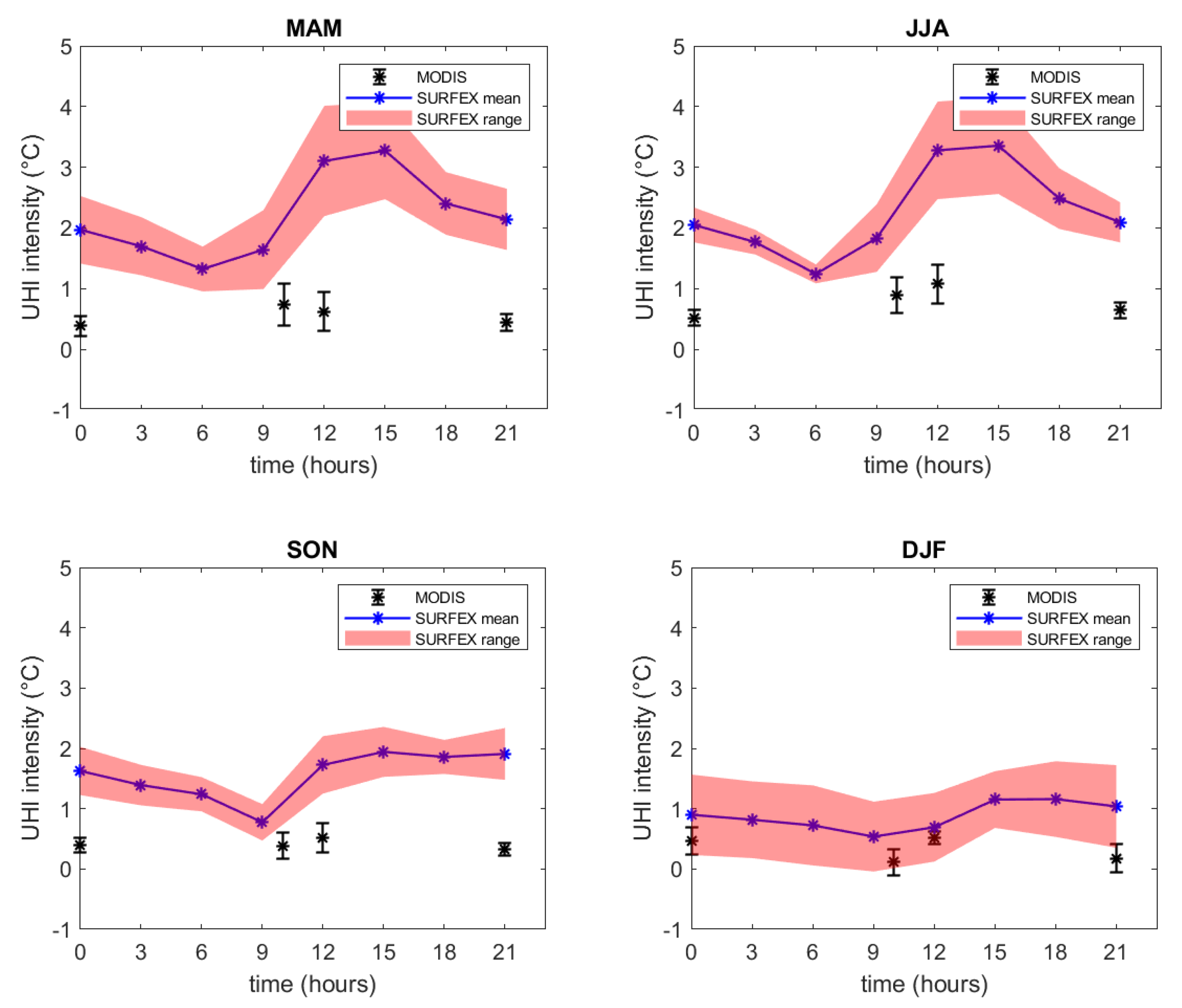
3.1. Surface Temperature and SUHI

Figure 3 shows the seasonal mean surface temperature in MODIS and in SURFEX-EI in daytime and nighttime (12 and 0 UTC in SURFEX, respectively).
Note that the surface temperature over the river is prescribed and kept constant throughout the simulation, therefore these gridpoints were masked out. Considering the nighttime results, the core of the city is emerging with the highest temperature in all seasons in SURFEX. This pattern can be detected in the observation too; however, it has different magnitude and shape. Generally, the isotherm lines portray roughly concentric circles around the downtown in the MODIS, while in SURFEX, except the warmest downtown area, the rest of the city is approximately equally warm. The spatial pattern of the observed daily SUHI largely differs from the nocturnal results, and the differences between the model and observation are larger as well. In MODIS, the hilly area of the domain (west from the Danube, mainly forests) is much colder than the plain areas from spring to autumn. The influence of topography and partly the cooling effect of trees on the daytime surface temperature can be seen in SURFEX as well, however over a smaller area, not propagating into the western edge of the city. Due to this orographic and land cover effect, the warmest area is observed over the Pest side of Budapest (east from the Danube), while in SURFEX almost the overall urban area is significantly warmer than its environment.
The daytime and nighttime land surface temperatures averaged over the urban and rural areas are seasonally shown on boxplots for SURFEX and MODIS (Figure 4) and temporally averaged values are shown in Table 3. The urban LST is overestimated almost in all seasons and in daytime and nighttime as well (as it was suggested earlier); while in winter, the model performs the best over the whole domain. The rural temperatures are colder in spring and autumn at night and in spring at noon in SURFEX than in MODIS, which-in line with the exaggerated urban temperatures-leads to stronger simulated SUHI. It can be also mentioned that variability is well described by the model with slightly overestimated variability of the mean urban temperature.
The SUHI-affected area was investigated and validated following the method of Zhang and Wang [47]. Figure 5 shows the seasonal distribution of the relative area of SUHI affected gridpoints (the sum of the gridpoints where T > T ¯ + σ ) over the city of Budapest. In MODIS at night the histograms are skewed left in each season except winter (when it is rather symmetric) with the most frequent values of 25–30%. The general overestimation of SUHI extent in SURFEX is obvious, because except winter the histogram is shifted towards the larger values. The most frequent SUHI area is between 35–40%, which occurs in the great majority of time in spring and summer. However, in winter, the histogram of SURFEX has a bimodal shape and most often the SUHI area is below 5%, therefore in this season MODIS shows a more developed SUHI area. At daytime, SURFEX shows a similar distribution to nighttime results both in the shape and most frequent SUHI relative area. While the histogram of observed value portrays different shape than at nighttime, because they are rather symmetric except summer (when it is skewed left). The most frequent areas are 10–30% that is lower than of SURFEX again. In winter the same can be observed, SURFEX underestimates the SUHI affected area. Based on this analysis we can conclude that there is much smaller variability in the SUHI affected area in SURFEX both at day and at night in all seasons compared to MODIS measurement.
Finally, the seasonal mean daily cycle of SUHI is shown in Figure 6. It is obvious that besides the general overestimation in SURFEX, there is a much larger intraday variability in LST compared to MODIS, especially in spring and summer. SUHI varies between 1 °C and 4 °C in spring and summer, 0.5 °C and 2 °C in autumn and 0.5 °C and 1 °C in winter in SURFEX, while in MODIS it does not exceed 1.5 °C in any seasons. The best agreement is found in winter at 12 and 0 UTC compared to the Aqua results.

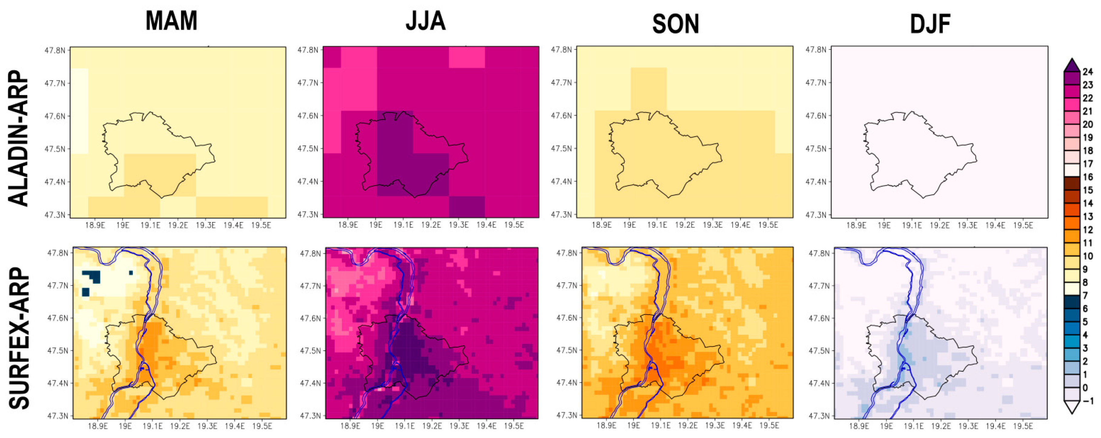
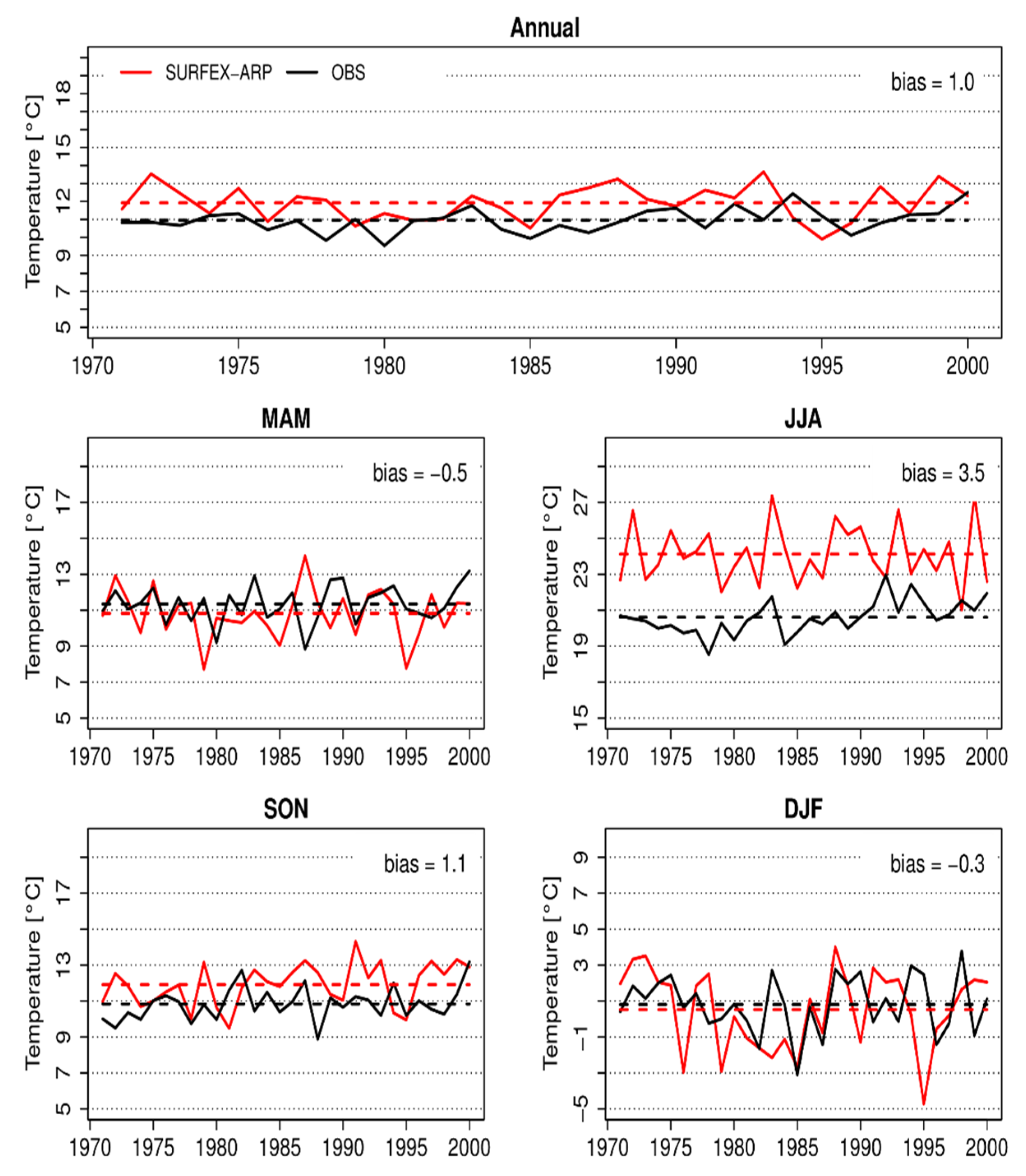
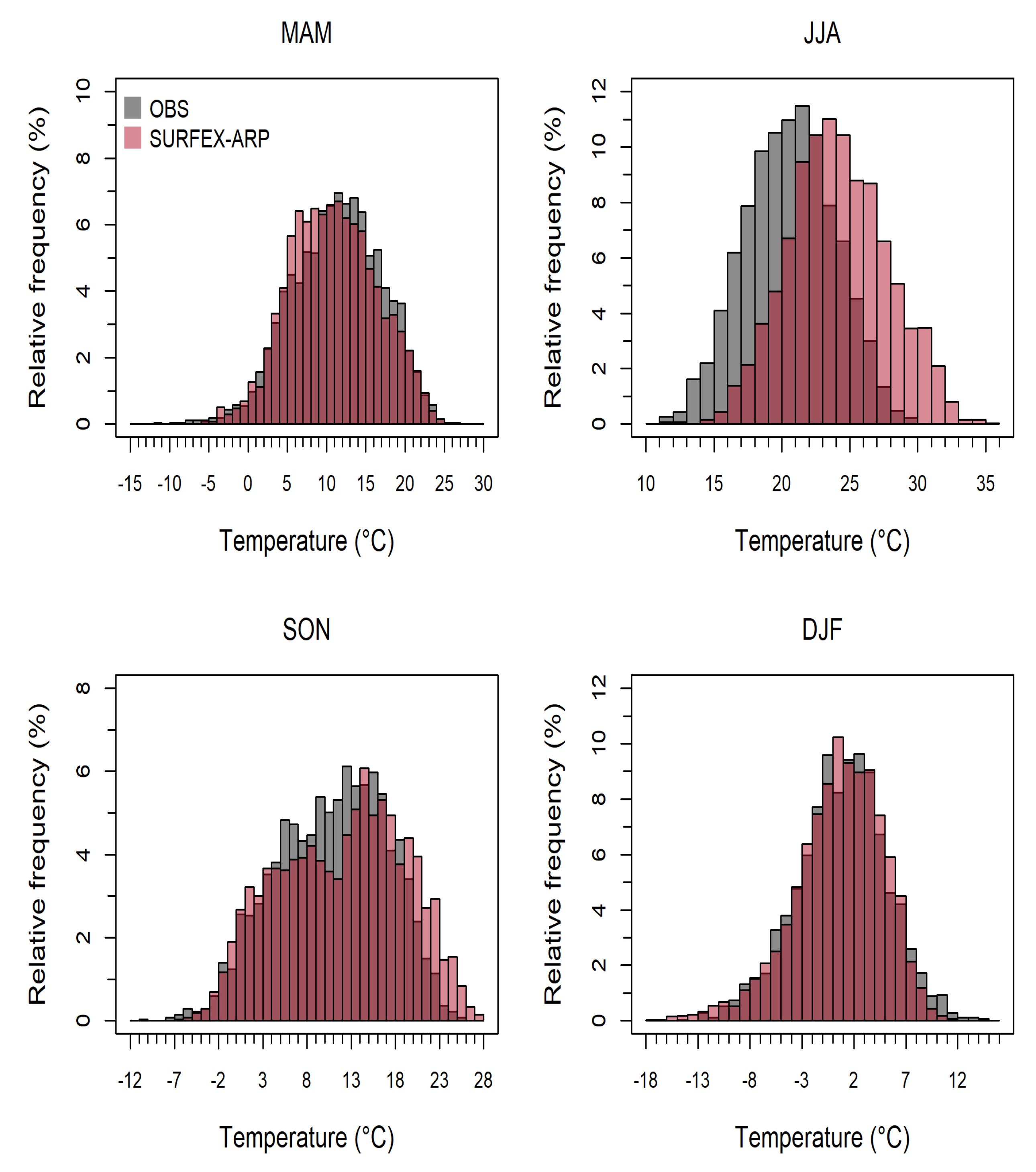
3.2. 2-m Temperature and UHI Climatology

In the following, 2 m temperature simulated by SURFEX-ARP is studied and compared in one suburban gridpoint with station measurements in the period of 1971–2000. Before the SURFEX results are assessed, it can be mentioned that the ALADIN (providing forcings to SURFEX) largely (with 2.9 °C) overestimates the 2 m temperature in summer, while underestimates it in the rest of the year over the SURFEX domain with respect to the 10 km resolution CarpatClim-Hu gridpoint dataset (Table 4).
Comparison of the 2 m temperature in ALADIN and SURFEX reveals that SURFEX heats not only the urban gridpoints (due to the detailed land cover and parameterization), but in autumn and in winter the lower elevated rural gridpoints are warmer as well (Figure 7). In the gridpoint nearest to the station located in the suburban area, SURFEX overestimates the measured value in summer and autumn, with 3.5 °C and 1.1 °C respectively (Figure 8). In spring and in winter smaller underestimation can be observed. The variance of the mean values are similar in SURFEX than the observation in the 30 year period, apart from summer, when SURFEX overestimates the interannual variability of the mean temperature (Table 5).
The seasonal distribution of daily temperatures is presented on histograms (Figure 9). In spring and winter the distributions of the simulated and observed temperature are in good agreement. In summer, the systematic overestimation is clear: the histogram based on SURFEX outputs has the same shape as the one based on the observations, but it is shifted towards higher values. The largest inconsistency is in autumn, when the model values show bimodal distribution, which (i.e., the lower occurrence of the values between the most frequent values) is not visible in the observation. The underestimation of the mean values can be explained with the higher frequency of higher temperature values.
The diurnal evolution of 2 m temperature in the suburban area is best simulated in spring and winter (Figure 10), especially at 0 and 12 UTC. However, in the morning hours the temperature is slightly underestimated, while in winter in the afternoon hours overestimation occurs too. In summer in addition to the general overestimation, the temperature after 15 UTC does not drop as fast as in the observation. Moreover, the lowest temperature is simulated to occur later at 6 UTC instead of 3 UTC (note, that data was available in 3 h frequency for both the observation and the simulation) and it increases faster in the morning compared to observations. In autumn a smaller overestimation is detected from noon to 6 UTC.

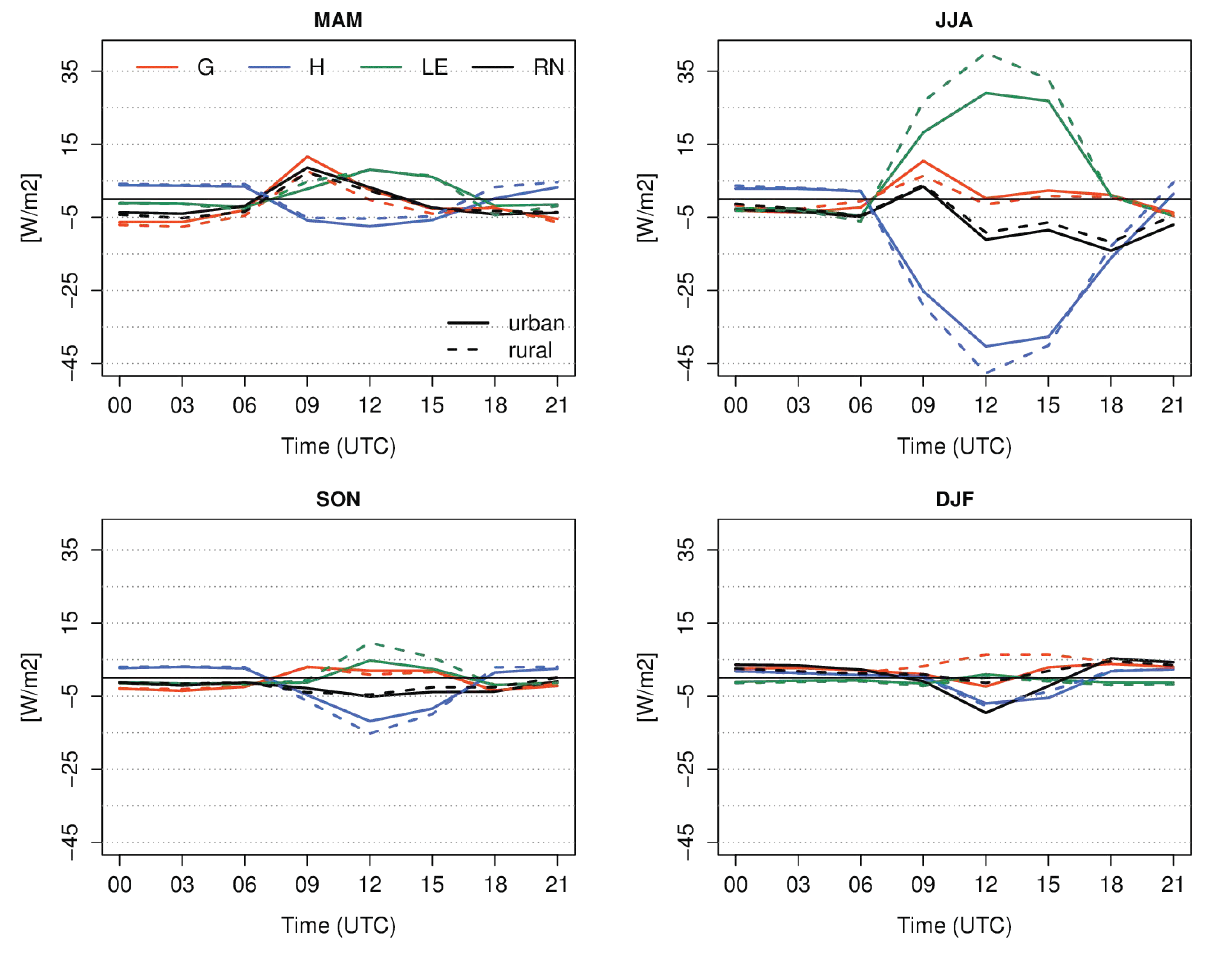
3.3. Comparison of SURFEX-EI and SURFEX-ARP for Simulating the UHI

Finally, the two experiments are compared on a common period (1996–2005) from the aspect of simulating UHI. Figure 11 presents the seasonal mean UHI at 0 UTC in SURFEX-EI and SURFEX-ARP. The differences are not large between the two simulations, however the GCM driven model gives stronger temperature surplus (with 0.1–0.2 °C) over the city than its reanalysis driven counterpart. Note that the differences for the 2-m temperature are much higher (e.g., the 2 m temperature bias is 1.1 °C and 2.5 °C for SURFEX-EI and SURFEX-ARP, respectively, compared to CarpatClim-HU over Budapest; not shown), but the subtraction in UHI eliminates the great majority of the systematic bias.
The reasons behind the stronger UHI in SURFEX-ARP can be explained by comparing the surface energy budget components (Figure 12). The ground heat flux over the urban surfaces is larger in SURFEX-ARP in the morning hours, while it is smaller during the night than in SURFEX-EI in all seasons except winter. Therefore, in the GCM driven experiment the city absorbs more heat during the day and emits more during the night that explains the stronger UHI. Moreover, less sensible heat and more latent heat are emitted in SURFEX-ARP than SURFEX-EI.

4. Discussion

The first part of this study focuses on the spatial and temporal characteristics of surface temperature and SUHI simulated by SURFEX-EI, considering the MODIS LST product as reference. The seasonal mean surface temperature is substantially warmer over the whole city than the ambient rural areas from spring to autumn, resulting in large SUHI extent and magnitude both at day and night. In contrast, MODIS shows that the highest temperature surplus of the city concentrates in the core of the city at night and in the Pest side (to the east of the Danube) by day. The less realistic variability and extent of SUHI in SURFEX can be explained partly by the lack of modelling the full boundary layer and its dynamics. Moreover, in the suburbs the canyon concept is less representative for the family houses than in the downtown area of the city. To solve this problem, the Local Climate Zone approach has been developed that classifies the urban areas based on compactness and height of buildings [48].
On the Buda side (west of Danube), the city is hilly and very green. Studies demonstrate that implementing trees in the urban canopy scheme can reduce surface temperature overestimation with several degrees [49,50]. These suggests that the strong summer and autumn surface temperature overestimation over the city (8.3 °C and 5.4 °C, respectively over the urbanized gridcells) and especially over Buda and the suburbs may be significantly lowered with a more explicit modelling of street trees’ effect.
The best agreement between the model and observation was found in winter, when surface temperature bias remains below 1 °C for urban and rural areas both at day and night. The small biases may be explained by that we only considered cloudy-free cases and in winter there is no leafy vegetation.
Upon SURFEX limitations, it is worth noting that satellite LST products are burdened with some considerable uncertainties [19,51] as well. For example, LST observations are valid only during clear-sky conditions, that limits the meteorological conditions to be potentially studied. In addition, satellite cloud-screening algorithms are often imperfect, causing biases in LST estimation [19]. Moreover, large viewing angles enhance atmospheric radiation extinction that can result in biases in observed LST [19,51,52]. Lastly, the anisotropy of LST (caused by the high level of surface heterogeneity particularly in urban areas) modifies the viewing angle of the satellite sensor above certain objects, hence leads to the uncertainty of observation as well [19]. Finally, it must be also mentioned, that since SURFEX results are saved 3-hourly, there is a 30–45 min difference between the compared simulation and the Aqua satellite’s observation time, that may contribute to a certain proportion of bias, especially during the day. Despite these limitations, the satellite observations provide important reference to assess the model’s ability to simulate spatial characteristics of urban temperature.
After the surface temperature and SUHI analysis in SURFEX-EI on shorter timescale, the 2 m temperature was studied in SURFEX-ARP for 30 years. The behavior of the driving ALADIN model strongly affects the results of SURFEX, i.e., the strong positive summer bias is dominantly caused by the 2.9 °C overestimation of ALADIN-Climate over the model domain. According to [49] the more explicit parameterization of street trees does not improve significantly the 2 m temperature overestimation of the LSM.
It was also found, that SURFEX heats not only the urbanized gridpoints, but in autumn and in winter the lower elevated rural areas as well. The surface scheme of ALADIN is also SURFEX version 5, but TEB and the SBL scheme was not activated in the climate change runs. Instead, the screen level values were computed by the Geleyn diagnostic formula [38]. One advantage of the SBL scheme is that it does not let the 2 m temperature cool too much in very stable situations, in order to prevent the decoupling of the surface model and the atmospheric component [31]. It was found in short term sensitivity studies that the minimum temperatures computed with the SBL scheme are higher compared to the diagnostic formula (not shown).
Apart from summer, the ALADIN-Climate is too cold compared to CarpatClim-HU. The majority of this cold bias was eliminated by SURFEX resulting smaller underestimation in spring and winter (less than 1.5 °C) and small positive bias in autumn (less than 1 °C) over the domain. The validation in the suburban gridpoint suggests that SURFEX is able to sufficiently describe the seasonal distribution of the daily mean temperature and the seasonal mean diurnal cycle. However, it must be mentioned that these investigations were achieved only in one gridpoint and more long term station measurement is needed to justify our results.
The limitations of ECOCLIMAP—i.e., it is a static database based on land cover data from the mid-90s—can also explain parts of the mean 2-m temperature bias of SURFEX-ARP. The importance of built-up fraction was studied in short sensitivity tests and was found that the bias originated from the driving model is more important. e.g., if the temperature is overestimated, reducing the urban fraction in the gridcell could moder-ate the bias; however, in other periods when the model is too cold, a smaller built-up ratio caused larger underestimation.
Comparing SURFEX-EI and SURFEX-ARP from the aspect of seasonal mean diurnal cycle of UHI, it can be stated that the systematic bias of the land surface model (and therefore the influence of the driving model) largely diminishes in the UHI.

5. Conclusions

The aim of this study was a thorough validation of the SURFEX LSM from the aspect of simulating surface and 2 m temperature and the corresponding UHI over Budapest. SURFEX was first forced by the ERA-Interim re-analysis driven ALADIN-Climate regional climate model, in order to reveal how the ALADIN-Climate model itself influences the LSM. Due to the strong correlation with observations, only a shorter 10-year past period was modelled, and the results were compared to the MODIS satellite LST observations for 2003–2005. It was found that the spatial extent of warmer area and even the location of heat island much more varies seasonally and between day and night in MODIS than in SURFEX. The surface temperature of SURFEX is much warmer over all the urban gridpoints than the measurement, resulting in larger SUHI extent from spring to autumn both at day and night. It was statistically underpinned that the daily variability of SUHI affected area is smaller than observed.
SURFEX was also forced by the GCM driven ALADIN-Climate model in the period of 1960–2005. The RCM was evaluated against the CarpatClim-Hu gridded observational dataset over the SUREX domain and 2 m temperature of SURFEX in one suburban gridpoint was validated with respect to station measurement for the period of 1971–2000. The main goal of this research was to assess the capability of SURFEX to simulate urban climate on decadal timescale. It was found that over the Budapest domain the ARPEGE driven ALADIN-Climate largely overestimates the temperature in summer, while underestimates it in the other seasons. This summer positive bias is inherited in SURFEX as well, leading to 3.5 °C warmer summer temperature compared to station measurement. In other seasons the difference between the land surface model and observation does not exceed 1.5 °C. The daily cycle of 2 m temperature is reasonably simulated and only smaller differences were found in each season except the systematic bias of summer. The long term gridpoint validation results of SURFEX are very promising, although to get more robust information a dense measurement network would be important.
Finally, the two experiments were compared on a common 10-year period from the aspect of simulating UHI. The spatial distribution and magnitude of UHI does not differ too much, because the majority of the systematic model bias is eliminated in the UHI calculation. However, small differences were found in the magnitude of the ground heat flux, that explains the small differences in the temperature excess over the city.

Author Contributions

Conceptualization, G.Z.; methodology, G.Z. and S.I.M.; formal analysis, G.Z. and S.I.M.; investigation, G.Z. and S.I.M.; data curation, G.Z. and S.I.M.; writing—original draft preparation, G.Z. and S.I.M.; writing—review and editing, G.Z. and S.I.M.; visualization, G.Z. and S.I.M.; project administration, G.Z.; funding acquisition, G.Z. All authors have read and agreed to the published version of the manuscript.

Funding

This research was funded by the KLIMADAT, grant number KEHOP-1.1.0-15-2015-00001 project.

Institutional Review Board Statement

Not applicable.

Informed Consent Statement

Not applicable.

Data Availability Statement

The ALADIN and SURFEX simulation data used in this study are stored locally at the Hungarian Meteorological Service and can be provided upon request. The CarpatClim-Hu dataset and the station measurements are available at http://odp.met.hu. MODIS Aqua, Terra and IGBP products were retrieved from NASA’s Land Processes Distributed Active Archive Center (https://lpdaac.usgs.gov/).

Acknowledgments

The ALADIN-Climate simulations were performed within the framework of the RCMGiS (EEA-C13-10) project. We acknowledge the use of MODIS Aqua and Terra land surface temperature imagery from NASA’s Land Processes Distributed Active Archive Center. We wish to say thanks to the Climate Division of the Hungarian Meteorological Service for providing the CarpatClim-Hu and station measurements. Great thanks are also dedicated for Gabriella Szépszó, who improved this paper with useful recommendations. Last but not least, the authors would like to express their gratitude to the three anonym reviewers for their detailed and valuable reviews.

Conflicts of Interest

The authors declare no conflict of interest. The funders had no role in the design of the study; in the collection, analyses, and interpretation of data; in the writing of the manuscript, and in the decision to publish the results.

References

  1. Oke, T.R. The energetic basis of the urban heat island. Q. J. R. Soc. Meteorol. Soc. 1982, 108, 1–24. [Google Scholar] [CrossRef]
  2. Elvidge, C.D.; Tuttle, B.T.; Sutton, P.C.; Baugh, K.E.; Howard, A.T.; Milesi, C.; Bhaduri, B.; Nemani, R. Global Distribution and Density of Constructed Impervious Surfaces. Sensors 2007, 7, 1962–1979. [Google Scholar] [CrossRef] [PubMed]
  3. Finta, S.; Maczák, J.; Kovács, B.; Mátrai, R. Budapest 2030; Long term urban development plan (in Hungarian). Municipality of Budapest Mayor’s Office: Budapest, Hungary, 2013. [Google Scholar]
  4. Revi, A.; Satterthwaite, D.E.; Aragón-Durand, F.; Corfee-Morlot, J.; Kiunsi, R.B.R.; Pelling, M.; Roberts, D.C.; Solecki, W. Urban areas. In Climate Change 2014: Impacts, Adaptation, and Vulnerability; Field, C.B., Barros, V.R., Dokken, D.J., Mach, K.J., Mastrandrea, M.D., Bilir, T.E., Chatterjee, M., Ebi, K.L., Estrada, Y.O., Genova, R.C., et al., Eds.; Part A: Global and Sectoral Aspects. Contribution of Working Group II to the Fifth Assessment Report of the Intergovernmental Panel on Climate Change; Cambridge University Press: Cambridge, UK; New York, NY, USA, 2014; pp. 535–612. [Google Scholar]
  5. Hoegh-Guldberg, O.; Jacob, D.; Taylor, M.; Bindi, M.; Brown, S.; Camilloni, I.; Diedhiou, A.; Djalante, R.; Ebi, K.L.; Engelbrecht, F.; et al. Impacts of 1.5 °C Global Warming on Natural and Human Systems. In Global Warming of 1.5 °C; An IPCC Special Report on the Impacts of Global Warming of 1.5 °C above Pre-Industrial Levels and Related Global Greenhouse Gas Emission Pathways, in the Context of Strengthening the Global Response to the Threat of Climate Change, Sustainable Development, and Efforts to Eradicate Poverty; Masson-Delmotte, V., Zhai, P., Pörtner, H.-O., Roberts, D., Skea, J., Shukla, P.R., Pirani, A., Moufouma-Okia, W., Péan, C., Pidcock, R., et al., Eds.; IPCC: Geneva, Switzerland, 2018. [Google Scholar]
  6. Oleson, K.W.; Bonan, G.B.; Feddema, J.; Jackson, T. An examination of urban heat island characteristics in a global climate model. Int. J. Climatol. 2011, 31, 1848–1865. [Google Scholar] [CrossRef] [Green Version]
  7. Katzfey, J.; Schlünzen, H.; Hoffmann, P.; Thatcher, M. How an urban parameterization affects a high-resolution global climate simulation. Q. J. R. Meteorol. Soc. 2020, 146, 3808–3829. [Google Scholar] [CrossRef]
  8. Daniel, M.; Lemonsu, A.; Déqué, M.; Somot, S.; Alias, A.; Masson, V. Benefits of explicit urban parameterization in regional climate modeling to study climate and city interactions. Clim. Dyn. 2019, 52, 2745–2764. [Google Scholar] [CrossRef] [Green Version]
  9. Hamdi, R.; Van de Vyver, H.; De Troch, R.; Termonia, P. Assessment of three dynamical urban climate downscaling methods: Brussels’s future urban heat island under an A1B emission scenario: Brussels’ future urban heat island. Int. J. Climatol. 2014, 34, 978–999. [Google Scholar] [CrossRef]
  10. Langendijk, G.S.; Rechid, D.; Jacob, D. Urban Areas and Urban–Rural Contrasts under Climate Change: What Does the EURO-CORDEX Ensemble Tell Us?—Investigating near Surface Humidity in Berlin and Its Surroundings. Atmosphere 2019, 10, 730. [Google Scholar] [CrossRef] [Green Version]
  11. Lin, C.-Y.; Chen, W.-C.; Chang, P.-L.; Sheng, Y.-F. Impact of the Urban Heat Island Effect on Precipitation over a Complex Geographic Environment in Northern Taiwan. J. Appl. Meteorol. Clim. 2011, 50, 339–353. [Google Scholar] [CrossRef]
  12. Grimmond, C.S.B.; Blackett, M.; Best, M.J.; Barlow, J.; Baik, J.-J.; Belcher, S.E.; Bohnenstengel, S.I.; Calmet, I.; Chen, F.; Dandou, A.; et al. The International Urban Energy Balance Models Comparison Project: First Results from Phase 1. J. Appl. Meteorol. Clim. 2010, 49, 1268–1292. [Google Scholar] [CrossRef]
  13. Hamdi, R.; Giot, O.; De Troch, R.; Deckmyn, A.; Termonia, P. Future climate of Brussels and Paris for the 2050s under the A1B scenario. Urban Clim. 2015, 12, 160–182. [Google Scholar] [CrossRef]
  14. Zsebeházi, G.; Szépszó, G. Modeling the urban climate of Budapest using the SURFEX land surface model driven by the ALADIN-Climate regional climate model results. Időjárás 2020, 124, 191–207. [Google Scholar] [CrossRef]
  15. Kotlarski, S.; Keuler, K.; Christensen, O.B.; Colette, A.; Déqué, M.; Gobiet, A.; Goergen, K.; Jacob, D.; Lüthi, D.; Van Meijgaard, E.; et al. Regional climate modeling on European scales: A joint standard evaluation of the EURO-CORDEX RCM ensemble. Geosci. Model Dev. 2014, 7, 1297–1333. [Google Scholar] [CrossRef] [Green Version]
  16. Cornes, R.C.; van der Schrier, G.; van den Besselaar, E.J.; Jones, P.D. An ensemble version of the E-OBS temperature and precipitation data sets. J. Geophys. Res. Atmos. 2018, 123, 9391–9409. [Google Scholar] [CrossRef] [Green Version]
  17. Bihari, Z.; Lakatos, M.; Szentimrey, T. Gridded observational datasets based on surface observations at the Hungarian Meteorological Service (in Hungarian). Légkör 2017, 62, 148–151. [Google Scholar]
  18. Oke, T.R. Initial guidance to obtain representative meteorological observations at urban sites. In WMO Instruments and Observing Methods; WMO/TD-No. 1250; IOM Report-No. 81; World Meteorological Organisation: Geneva, Switzerland, 2006. [Google Scholar]
  19. Hu, L.; Brunsell, N.A.; Monaghan, A.J.; Barlage, M.; Wilhelmi, O.V. How can we use MODIS land surface temperature to validate long-term urban model simulations? J. Geophyss. Res. Atmos. 2014, 119, 3185–3201. [Google Scholar] [CrossRef] [Green Version]
  20. Caluwaerts, S.; Hamdi, R.; Top, S.; Lauwaet, D.; Berckmans, J.; Degrauwe, D.; Dejonghe, H.; De Ridder, K.; De Troch, R.; Duchêne, F.; et al. The Urban Climate of Ghent, Belgium: A Case Study Combining a High-Accuracy Monitoring Network with Numerical Simulations. Urban Clim. 2020, 31, 100565. [Google Scholar] [CrossRef]
  21. Muller, C.L.; Chapman, L.; Grimmond, C.S.B.; Young, D.T.; Cai, X. Sensors and the city: A review of urban meteorological networks. Int. J. Climatol. 2013, 33, 1585–1600. [Google Scholar] [CrossRef]
  22. Unger, J.; Savic, S.; Gál, T.; Milosevic, D. Urban Climate and Monitoring Network System in Central European Cities; European Union: Novi Sad, Serbia, 2014; 101p, ISBN 987-86-7031-341-5. [Google Scholar]
  23. Le Roy, B.; Lemonsu, A.; Kounkou-Arnaud, R.; Brion, D.; Masson, V. Long time series spatialized data for urban climatological studies: A case study of Paris, France. Int. J. Climatol. 2020, 40, 3567–3584. [Google Scholar] [CrossRef]
  24. Tomlinson, C.J.; Chapman, L.; Thornes, J.E.; Baker, C. Remote sensing land surface temperature for meteorology and climatology: A review. Meteorol. App. 2011, 18, 296–306. [Google Scholar] [CrossRef] [Green Version]
  25. Hamdi, R.; Van de Vyver, H. Estimating urban heat island effects on near-surface air temperature records of Uccle (Brussels, Belgium): An observational and modeling study. Adv. Sci. Res. 2011, 6, 27–34. [Google Scholar] [CrossRef] [Green Version]
  26. Masson, V.; Le Moigne, P.; Martin, E.; Faroux, S.; Alias, A.; Alkama, R.; Belamari, S.; Barbu, A.; Boone, A.; Bouyssel, F.; et al. The SURFEXv7.2 Land and Ocean Surface Platform for Coupled or Offline Simulation of Earth Surface Variables and Fluxes. Geosci. Model Dev. 2013, 6, 929–960. [Google Scholar] [CrossRef] [Green Version]
  27. Masson, V.; Champeaux, J.-L.; Chauvin, F.; Meriguet, C.; Lacaze, R. A Global Database of Land Surface Parameters at 1-Km Resolution in Meteorological and Climate Models. J. Clim. 2003, 16, 1261–1282. [Google Scholar] [CrossRef]
  28. Boone, A.; Calvet, J.-C.; Noilhan, J. Inclusion of a Third Soil Layer in a Land Surface Scheme Using the Force–Restore Method. J. Appl. Meteorol. 1999, 38, 1611–1630. [Google Scholar] [CrossRef]
  29. Masson, V. A Physically-Based Scheme for The Urban Energy Budget In Atmospheric Models. Bound. Lay. Meteorol. 2000, 94, 357–397. [Google Scholar] [CrossRef]
  30. Hamdi, R.; Masson, V. Inclusion of a Drag Approach in the Town Energy Balance (TEB) Scheme: Offline 1D Evaluation in a Street Canyon. J. Appl. Meteorol. Clim. 2008, 47, 2627–2644. [Google Scholar] [CrossRef] [Green Version]
  31. Masson, V.; Seity, Y. Including Atmospheric Layers in Vegetation and Urban Offline Surface Schemes. J. Appl. Meteorol. Clim. 2009, 48, 1377–1397. [Google Scholar] [CrossRef]
  32. Colin, J.; Déqué, M.; Radu, R.; Somot, S. Sensitivity Study of Heavy Precipitation in Limited Area Model Climate Simulations: Influence of the Size of the Domain and the Use of the Spectral Nudging Technique. Tellus A 2010, 62, 591–604. [Google Scholar] [CrossRef] [Green Version]
  33. Voldoire, A.; Sanchez-Gomez, E.; Salas y Mélia, D.; Decharme, B.; Cassou, C.; Sénési, S.; Valcke, S.; Beau, I.; Alias, A.; Chevallier, M.; et al. The CNRM-CM5.1 Global Climate Model: Description and Basic Evaluation. Clim. Dyn. 2013, 40, 2091–2121. [Google Scholar] [CrossRef] [Green Version]
  34. Mlawer, E.J.; Taubman, S.J.; Brown, P.D.; Iacono, M.J.; Clough, S.A. Radiative Transfer for Inhomogeneous Atmospheres: RRTM, a Validated Correlated-k Model for the Longwave. J. Geophys. Res. 1997, 102, 16663–16682. [Google Scholar] [CrossRef] [Green Version]
  35. Fouquart, Y.; Bonnel, B. Computations of solar heating of the earth’s atmosphere: A new parameterization. Beitr. Phys. Atmosph. 1980, 53, 35–62. [Google Scholar]
  36. Smith, R.N.B. Scheme for Predicting Layer Clouds and Their Water Content in a General Circulation Model. Q. J. R. Meteorol. Soc. 1990, 116, 435–460. [Google Scholar] [CrossRef]
  37. Bougeault, P. A Simple Parameterization of the Large-Scale Effects of Cumulus Convection. Mon. Weather Rev. 1985, 113, 2108–2121. [Google Scholar] [CrossRef] [Green Version]
  38. Geleyn, J.-F. Interpolation of Wind, Temperature and Humidity Values from Model Levels to the Height of Measurement. Tellus A 1988, 40A, 347–351. [Google Scholar] [CrossRef]
  39. Dee, D.P.; Uppala, S.M.; Simmons, A.J.; Berrisford, P.; Poli, P.; Kobayashi, S.; Andrae, U.; Balmaseda, M.A.; Balsamo, G.; Bauer, P.; et al. The ERA-Interim Reanalysis: Configuration and Performance of the Data Assimilation System. Q. J. R. Meteorol. Soc. 2011, 137, 553–597. [Google Scholar] [CrossRef]
  40. Wan, Z.; Hook, S.; Hulley, G. MOD11A1 MODIS/Terra Land Surface Temperature/Emissivity Daily L3 Global 1 km SIN Grid V006 LST_Day_1km, Day_View_Time, LST_Night_1km, Night_view_time. NASA EOSDIS Land Process DAAC 2015. [Google Scholar] [CrossRef]
  41. Wan, Z.; Hook, S.; Hulley, G. MYD11A1 MODIS/Aqua Land Surface Temperature/Emissivity Daily L3 Global 1km SIN Grid V006 LST_Day_1km, Day_View_Time, LST_Night_1km, Night_view_time. NASA EOSDIS Land Processes DAAC 2015. [Google Scholar] [CrossRef]
  42. Justice, C.O.; Townshend, J.R.G.; Vermote, E.F.; Masuoka, E.; Wolfe, R.E.; Saleous, N.; Roy, D.P.; Morisette, J.T. An overview of MODIS Land data processing and product status. Remote Sens. Environ. 2002, 83, 3–15. [Google Scholar] [CrossRef]
  43. Wan, Z.; Dozier, J. A generalized split-window algorithm for retrieving land-surface temperature from space. IEEE T. Geosci. Remote 1996, 34, 892–905. [Google Scholar] [CrossRef] [Green Version]
  44. Cover, M.L.; Change, L.C. MODIS Land Cover Product Algorithm Theoretical Basis Document (ATBD) Version 5.0. MODIS Documentation; Boston University: Boston, MA, USA, 1999; pp. 42–47. [Google Scholar]
  45. Friedl, M.; Sulla-Menashe, D. MCD12Q1 MODIS/Terra+Aqua Land Cover Type Yearly L3 Global 500m SIN Grid V006 LC_Type1. NASA EOSDIS Land Processes DAAC 2019. Available online: https://doi.org/10.5067/MODIS/MCD12Q1.006 (accessed on 28 July 2020).
  46. Szentimrey, T. Development of MASH homogenization procedure for daily data. In Proceedings of the Fifth Seminar for Homogenization and Quality Control in Climatological Databases, Budapest, Hungary, 29 May–2 June 2006. [Google Scholar]
  47. Zhang, J.; Wang, Y. Study of the Relationships between the Spatial Extent of Surface Urban Heat Islands and Urban Characteristic Factors Based on Landsat ETM+ Data. Sensors 2008, 8, 7453–7468. [Google Scholar] [CrossRef]
  48. Stewart, I.D.; Oke, T.R. Local Climate Zones for Urban Temperature Studies. Bull. Am. Meteorol. Soc. 2012, 93, 1879–1900. [Google Scholar] [CrossRef]
  49. Redon, E.; Lemonsu, A.; Masson, V. An urban trees parameterization for modeling microclimatic variables and thermal comfort conditions at street level with the Town Energy Balance model (TEB-SURFEX v8.0). Geosci. Model Dev. 2020, 13, 385–399. [Google Scholar] [CrossRef] [Green Version]
  50. Wang, C.; Wang, Z.-H.; Ryu, Y.-H. A single-layer urban canopy model with transmissive radiation exchange between trees and street canyons. Build. Environ. 2021, 191, 107593. [Google Scholar] [CrossRef]
  51. Ghent, D.; Veal, K.; Trent, T.; Dodd, E.; Sembhi, H.; Remedios, J. A new approach to defining uncertainties for MODIS land surface temperature. Remote Sens. 2019, 11, 1021. [Google Scholar] [CrossRef] [Green Version]
  52. Freitas, S.C.; Trigo, I.F.; Bioucas-Dias, J.M.; Gottsche, F.M. Quantifying the uncertainty of land surface temperature retrievals from SEVIRI/Meteosat. IEEE Trans. Geosci. Remote Sens. 2009, 48, 523–534. [Google Scholar] [CrossRef] [Green Version]
Figure 1. Flow chart about the use of SURFEX. Upper panel: domain and orography of the 10 km resolution ALADIN-Climate and its selected part covering Budapest, for which model fields are interpolated to 1 km resolution. Lower panel: land cover types according to the ECOCLIMAP database for the Budapest domain. Black X marks the closest gridpoint to the considered station measurement, which is also shown on orthophoto on the lower left corner (Google Earth image).
Atmosphere 12 00709 g001
Figure 2. Land-use types for Budapest metropolitan area based on MODIS Land Cover Products. Blue rectangle represents the area that was considered for computing the SUHI affected area.
Atmosphere 12 00709 g002
Figure 3. Seasonal mean land surface temperature (°C) in MODIS and radiative temperature in ALAD-EI driven SURFEX at 00 and 12 UTC in 2003–2005. Surface temperature over the Danube is masked out in the SURFEX results.
Atmosphere 12 00709 g003
Figure 4. Box-whisker diagram of nighttime and daytime LST (°C) averaged over the urban and rural gridpoints in MODIS and SURFEX. Period: 2003–2005. The lower and upper boundaries of the boxes represent the lower and upper quartiles of the distribution, while the extent of the whiskers shows the minimum and maximum values. The median is represented by horizontal lines inside the boxes.
Atmosphere 12 00709 g004
Figure 5. Histogram of relative SUHI affected area (compared to the total domain) at nighttime (top) and daytime (bottom) in each season in 2003–2005 over the city of Budapest.
Atmosphere 12 00709 g005
Figure 6. Seasonal mean SUHI (°C, black and blue dots) daily cycle based on 3 h data of SURFEX and 4 measurements of MODIS per day in 2003–2005. The standard deviation of the daily values is indicated with whiskers for MODIS and pink band for SURFEX.
Atmosphere 12 00709 g006
Figure 7. Seasonal mean 2 m temperature (°C) in ALADIN-ARP (first row) and SURFEX-ARP (second row) for the period of 1971–2000.
Atmosphere 12 00709 g007
Figure 8. Annual and seasonal 2 m temperature (°C) of SURFEX-ARP in the suburban gridpoint and of the suburban station (Pestszentlőrinc) between 1971 and 2000. The 30 year average is marked with dashed lines and the mean bias indicated in the upper right corner.
Atmosphere 12 00709 g008
Figure 9. Histogram of daily 2-m temperature (°C) in each season according to SURFEX-ARP and station measurement in 1971–2000.
Atmosphere 12 00709 g009
Figure 10. Seasonal mean daily cycle of 2 m temperature (°C) according to SURFEX (red line) and observation (black line with dots). The pink area and the black vertical lines represent the standard deviation computed from the yearly values. Period: 1971–2000.
Atmosphere 12 00709 g010
Figure 11. Seasonal mean urban heat island intensity (°C) based on SURFEX-EI and SURFEX-ARP for the period of 1996–2005. The spatial averages of the urban gridpoints are indicated above the corresponding maps.
Atmosphere 12 00709 g011
Figure 12. Difference (W/m2) of the seasonal mean diurnal cycle of surface energy budget components (RN: net radiation, H: sensible heat flux, LE: latent heat flux, G: ground heat flux) for the urban and rural grid points between the SURFEX-ARP and SURFEX-EI experiment. Period: 1996–2005.
Atmosphere 12 00709 g012
Table 1. The overpass time in UTC of MODIS satellites.
AquaTerra
Day11:309:54
Night0:4320:42
Table 2. Main characteristics of the different reference datasets used for validation.
ReferenceResolutionTemporal FrequencyInvestigation PeriodValidated Variable
MODIS1 km4 times/day2003–2005LST, SUHI
CarpatClim-Hu10 kmdaily1971–20002 m temperature
Station measurement-daily, 3 h1971–20002 m temperature
Table 3. Seasonal mean urban and rural temperature (°C) in MODIS and SURFEX at nighttime and daytime in 2003–2005.
Nighttime (around 00 UTC)Daytime (around 12 UTC)
MAMJJASONDJFMAMJJASONDJF
RuralMODIS3.414.45.9−7.924.631.918.71.7
SURFEX2.816.95.3−7.118.635.722.02.6
UrbanMODIS4.715.77.0−6.426.334.720.02.5
SURFEX6.821.08.4−5.925.543.025.43.3
Table 4. Seasonal mean temperature bias (°C) of ALADIN-ARP and SURFEX-ARP with respect to the CarpatClim-Hu database on the SURFEX domain. All datasets were interpolated to the 10 km resolution CarpatClim-Hu grid. Period: 1971–2000.
AnnualMAMJJASONDJF
ALADIN-ARP−0.4−2.02.9−0.7−2.0
SURFEX-ARP0.4−1.23.00.6−0.7
Table 5. Standard deviation (°C) of annual and seasonal yearly 2 m temperature of SURFEX-ARP and of the suburban station measurement (Pestszentlőrinc) in 1971–2000.
AnnualMAMJJASONDJF
Observation0.71.00.90.91.6
SURFEX-ARP1.01.41.71.21.7
Publisher’s Note: MDPI stays neutral with regard to jurisdictional claims in published maps and institutional affiliations.

