Impact of Ragweed Pollen Daily Release Intensity on Long-Range Transport in Western Europe

Abstract

This study is dedicated to improving the daily release of ragweed pollen emission in the context of deterministic regional modelling for analysis and forecast. First, correlations are calculated between daily modelled meteorological variables (wind speed, temperature, humidity, precipitation, surface fluxes) and daily pollen counts at nine stations in Hungary, Croatia and France between 2005 and 2011. The 2 m temperature is the most correlated parameter, followed by convective velocity and incoming shortwave radiation, while precipitation rate and 2 m specific humidity act as limiting factors. Using these results, a ragweed pollen daily release formulation is proposed. This formulation is implemented in the CHIMERE chemistry-transport model and tested during the whole year of 2010. Results are compared to observations, and it is shown that the new formulation provides a more realistic day-to-day variability: the spatio-temporal correlation between surface measurements and modelled concentrations is 0.77, greater than two other known emission schemes.

1. Introduction

The Ambrosia artemisiifolia L. or common ragweed is an invasive weed, recognised for its atopic properties. For both event analysis and operational forecast, numerous efforts have been devoted to model its emission and transport. A recent overview of ragweed studies [1] showed that ragweed modelling is conducted using local statistical models (using observed meteorological data, for example), trajectories models, multi-parameter regression analyses, as well as regional models. While the physics of birch and ragweed pollen emissions is completely different, some models use the same physical basis to estimate these two different release terms, as in [2], for example.

Assessing and predicting ragweed pollen emissions is challenging because they are sensitive to many different biological and meteorological factors. First, even though major efforts are currently made (see, e.g., refs. [3,4]), the location of ragweed plants is difficult to establish, as presented in ref. [5] for France, in ref. [6] for Serbia, refs. [7,8] in Western Europe. Second, for an area with clearly identified ragweed, seasonal weather conditions determine the phenology of the plant and its pollen production. Depending on these seasonal conditions, the yearly amount of pollen may be very different from one year to another [9]. Finally, if the plants are present and climate conditions are favourable to the plant growth and flowering, hourly meteorological variability strongly influences the pollen release. A wealth of observational data were analysed to better understand the physical mechanisms underlying pollen emissions. One of the first foundational works is [10] studying pollen release in the common ragweed. A few years later, Holmes et al. [11] made measurements of hourly ragweed pollen concentrations during the summer of 1961 in Ottawa. For the first time, meteorological variables (relative humidity and air temperature) were measured together with ragweed pollen concentrations. It was shown that concentrations exhibited a diurnal peak during the morning when relative humidity suddenly decreased and temperature increased, except for the rainy days. No significant relationship with wind speed was found. The diurnal cycle of ragweed pollen was also studied by ref. [12].

What are the main drivers for ragweed pollen emissions? To answer this question, several studies were conducted in the last few decades. Laaidi et al. [13] analysed the ragweed pollen concentration data in Lyon (France) during the long-term period of 1987 to 1999. Using a statistical approach to relate meteorology and concentrations using a multi-parameter regression, they were able to predict the pollen season start with an error of 3 days at the maximum, and the duration of the pollen season with an error of 7 days at the maximum. The temperature range seems to be an important control factor, indicating the dehydration of pollens during the day, losing mass and thus more likely to be emitted under specific wind conditions. Makra et al. [14] also analysed observational data and studied a possible relationship between ragweed pollen and meteorology for the period of 1997 to 2001 and in the city of Szeged (Hungary). They used 11 meteorological variables and proposed a complex relation to fit their data. A similar approach is presented in ref. [15] over Rzeszow (Poland), quantifying the impact of temperature and wind speed on ragweed emissions. The strength of such studies is that they are close to the processes and are able to evaluate emissions taking into account the spatial representativeness of the measured concentrations. More recently, Matyasovszky et al. [7] conducted a statistical study to identify the main drivers leading to ragweed pollen emissions, more precisely, the season start and end in Europe. They found a clear relationship between the date of the last frost day and the maximum amount of emitted pollen grains.

Regional modelling was initiated to better understand, quantify and predict the individual processes driving concentration variability (emission fluxes, long-range transport, deposition). It has motivated the development of pollen emission parameterizations. Over recent years, a few schemes have been proposed to estimate the pollen emission fluxes. Helbig et al. [16] proposed a scheme for pollen emission and re-suspension with the KAMM/DRAIS model. In their model, pollen emissions are computed using a “characteristic” concentration (the sum of grains measured over one season), the leaf area index of the corresponding model grid cell and the friction velocity u${}_{*}$ acting as a limiting factor. Pollen emissions are considered as a threshold process, similar to the saltation of mineral dust over arid areas. That is why resistances based on relative humidity and wind speed are included. Zink et al. [17] used the Consortium for Small-scale Modelling (COSMO-ART) model to analyse a pollen episode observed over northern Germany in September 2006. They compared the local contribution and the import from Hungary (one of the European countries most exposed to ragweed spread) and found that at least 20% of the pollen counts could be attributed to transboundary inflow. Makra et al. [18] found that the annual ragweed pollen amount transported by the atmospheric circulation is 27.8% of the annual total pollen at Szeged (Hungary). From this quantity, 7.5% is added to (due to transport), while 20.3% is subtracted from (e.g., because of wash-out by frontal rainfalls going towards Szeged) local sources. Sofiev et al. [19] presented the first birch pollen forecast model, integrated into the SILAM model (System for Integrated Modelling of Atmospheric Composition) and applied it over the whole of Western Europe. The emissions were statistically prescribed. A few years later, Sofiev et al. [20] presented a deterministic emission module, with the flowering season driven by the heat sum, including a probabilistic term. The module was limited to birch pollen emissions. Efstathiou et al. [21] recently implemented a modified [16] scheme in CMAQ and modelled the pollen period of 2002 over Newark (United States, NJ). Zink et al. [2] presented a tunable scheme for different kinds of pollen (birch, ragweed). This scheme corresponds to the best fit between modelled emissions and recorded concentrations over several sites in Europe. However, correlations between observations and simulations were found to be insignificant. Prank et al. [22] proposed a scheme for ragweed emissions dedicated to pollen forecasts. Chapman et al. [4] modelled the ragweed spatial distribution and its evolution in the United States and in Europe. They showed that the phenology is able to correctly reproduce the propagation of this invasive plant. Liu et al. [23] also implemented a modified version of the ref. [16] scheme in the RegCM model with some surface characteristics determined using the CLM4.5 model. Regional models are now running together for daily forecast (the CAMS project) and for birch pollen, as explained in ref. [24]: the models are CHIMERE, EMEP, EURAD-IM (EURopean Air Pollution Dispersion), LOTOS-EUROS, MATCH, MOCAGE (Modèle de Chimie Atmosphérique de Grande Echelle) and SILAM. Multi-model ensembles are also performed with numerous models as in ref. [25] for olive pollen.

The main goal of this study is to quantify the impact of meteorological variables on ragweed pollen emission, more specifically the daily release. First, several meteorological variables are compared to local observations to identify possible correlations. Since collocated pollen-weather observations, including a consistent set of weather variables, are generally not available, we use here outputs from a mesoscale meteorological model. For representativeness and accuracy reasons, the low-resolution meteorological model can deviate from the actual meteorological context of the observation site. However, it remains the best available method to assess the capability of such regional models to calculate pollen concentrations over large areas, for past, present, and future studies (such as climate scenario studies). The observations from 2005 to 2011 and the model used are described in Section 2. The meteorological fields used are described in Section 3.1. Correlations between measured pollen counts and several modelled meteorological variables are presented in Section 3.3. The main rationale for pollen emission models is presented in Section 4. Among all processes for ragweed emissions, we focus on the daily release. In order to test an alternative formulation for this daily release, we implemented several schemes in the CHIMERE chemistry-transport model: (i) the SILAM model scheme [20], (ii) the [21] scheme and (iii) the new release term proposed in this study. The whole year of 2010 is modelled over Western Europe, and the modelled results are compared to measurements in Section 5. Finally, conclusions and perspectives are proposed in Section 6.

2. Methodology

In this study, the methodology follows threes steps:

• Statistical analysis over several years: We first want to quantify the impact of meteorological variables on ragweed pollen emissions. We compare pollen grains measurememnts with meteorological data. The studied period ranges from 2005 to 2011 with data from 9 stations.
• Definition of a new release term for a pollen emissions parametrization: Inspired by the results of the statistical scores, we define a new release term for ragweed pollen emission. The formulation is simple and only has the goal of giving more weight to the most sensitive meteorological parameters.
• Regional modelling of ragweed pollen emissions and transport: In order to quantify the interest of this new formulation, a regional simulation is performed for the period of February to October 2010. The year is selected because this is the period with the largest amount of measurement data.

2.1. The Link between the Several Measurements: Pollen and Meteorological Data

As for many geophysical studies, such as air quality (see ref. [26] among others), there is no possible direct measurements of emissions, only concentrations in the air. This means that when we want to estimate the realism of a new emissions scheme, there is no real constraint. The only way to have a “validation” is not direct and consists of comparing observed versus modelled concentrations. In this case, it is not only the emissions that are tested but also all other processes (transport, deposition).

In the case of the pollen, we assume that local emissions and pollen counts may be different, as has been shown in ref. [27]: a large maximum of pollen counts may occur due to local emissions and transport from around 50–100 km away, and it is difficult to separate these two contributions. At the local scale, several studies were devoted to this important point and developed methodologies to identify the origin of pollutants concentrations, such as ref. [28] for the identification of local sources of olive pollen, ref. [29] for the quantification of the impact of landuse and wind direction on local pollen concentrations and ref. [30], which proposed a new index to classify the several kinds of measured pollen grains.

For this study, we selected stations located in areas highly infested by ragweed pollen. Our assumption is, thus, that in most highly infested areas, daily pollen counts should be roughly proportional to emissions within a corresponding spatial scale. This spatial scale depends on many factors, including the local meteorology, the landuse and the pollen taxa [31,32]. Since we are aiming at modelling daily variability, our approach also considers a spatial scale of changes that is associated with this time scale. Considering a mean boundary layer wind of about 5 m/s, the transport of pollen but also weather variables within a distance of 100 km takes about 6 h, so our model aims indeed at being representative of this spatial scale (0–100 km) [33,34]. The use of pollen counts as a proxy is not new, for instance, a recent inventory of ragweed plants used counts to spatialise the presence of ragweed (together with other information) [35]. This is quite appropriate in the absence of flux data, as long as this assumption is clearly stated and kept in mind.

2.2. The Available Pollen Grains Measurements

Methodologies of pollen counting have been developed for several decades, such as in ref. [36]. Laaidi et al. [13] describes the main principle of Hirst volumetric traps, calibrated to handle flows of 10 L/min of air. The sampler is always oriented in the main wind direction and would be representative within a 30-km radius. Pollen grains are impacted on a cylinder covered by a plastic film: the grains are manually counted using a light microscope. Galán et al. [37] proposed a methodology to define the minimum requirements and reproducibility of analysis of pollen grains measurements.

Nine observation sites are used in this study, and their locations are given in

Table 1. List of all Ambrosia measurement stations used in this study. The stations of Debrecen, Györ and Zagreb are operated by the EAN network, the stations of Velika, Samobor, Ivanic, Slavonski and Bjelovar are operated by the HRTEAM network and the station of Roussillon by the RNSA network. For each year, the percentage of available data is given.

Station	City /Country	Longitude (°W)	2005	2006	2007	2008	2009	2010	2011
		Latitude (°N)	%	%	%	%	%	%	%
HUDEBR	Debrecen/Hungary	21.58/47.53	90	92	84	92	92	100	98
HUGYOE	Györ/Hungary	17.60/47.67	90	92	92	92	100	100	100
HRZAGR	Zagreb/Croatia	16.00/45.80	83	76	100	81	70	96	88
VELIKA	Velika-Gorica/ Croatia	16.38/45.78	0	0	0	100	100	83	100
SAMOBOR	Samobor/ Croatia	15.71/45.80	0	0	0	100	100	100	82
IVANIC	Ivanić-Grad/Croatia	16.07/45.70	0	0	0	100	82	100	100
SLAVONSKI	Slavonski Brod/Croatia	18.02/45.15	0	0	0	100	100	100	100
BJELOVAR	Bjelovar/Croatia	16.84/45.89	100	100	100	100	100	100	0
ROUSSILLON	Lyon/France	4.81/45.37	77	75	83	71	82	71	89

. The selection of the sites was based on the availability of 33 sites across Europe at the time of the study and on the basis of the mean pollen load. Most loaded sites were selected in order to have a set of sites where the fraction of count due to local emissions is maximised vs. regional transport. These sites are located in Croatia (HR), Hungary (HU) and France (FR). Sites were also selected for their satisfactory data completeness (from 71% to 100%). For each year and each station, the percentage of available data is given in Table 1. Note that for the stations VELIKA, SAMOBOR, IVANIC, and SLAVONSKI, there are no observations for the years 2005 to 2007. The measurements were collected from various institutes, but all data were quality-controlled and homogenised in the framework of the FP7 ATOPICA project [38].

2.3. Estimation of the Pollen Emissions Period

The first use of these data is to quantify the start and end dates of the pollen emissions. Having many years of data available, it is possible to quantify the inter-annual variability of these emissions periods. Many ways exist to define pollen season, as described in refs. [39,40]. As the process of measurements may be uncertain by a few per cent and to ensure the use of the correct pollen emission period, we selected the beginning and ending days as the 5% and 95% observed concentrations [13]. The results are presented in

Table 2. Julian day for the start of the pollen season (day when 5% of the annual pollen sum is reached) and number of days of the season (between 5% and 95% of the annual pollen sum). The empty lines are for stations and years with no data, as explained in Table 1.

Station	2005	2006	2007	2008	2009	2010	2011
BJELOVAR	229 + 29	230 + 29	226 + 33	225 + 29	223 + 33	227 + 30	-
HRZAGR	230 + 26	229 + 29	222 + 37	232 + 21	224 + 27	224 + 39	229 + 27
HUDEBR	219 + 43	228 + 45	218 + 49	223 + 34	226 + 31	227 + 30	224 + 42
HUGYOE	223 + 36	231 + 45	226 + 41	224 + 33	223 + 39	227 + 41	230 + 30
IVANIC	-	-	-	224 + 30	222 + 31	231 + 25	230 + 38
ROUSSILLON	227 + 33	230 + 25	224 + 35	229 + 26	224 + 34	230 + 31	222 + 35
SAMOBOR	-	-	-	228 + 30	225 + 29	232 + 41	230 + 39
SLAVONSKI	-	-	-	223 + 33	224 + 39	230 + 29	228 + 32
VELIKA	-	-	-	224 + 30	222 + 32	230 + 26	230 + 27

for each station and each year. We can notice some variability from year to year and over all stations: the pollen season starting date can vary up to 8 days, while the pollen season duration ranges from 21 to 49 days.

3. The Link between Pollen Concentration and Meteorology

In this section, we try to establish a link between the observed surface pollen concentration and the meteorology modelled for the corresponding location of the measurement. This link is searched by comparing daily data for those variables: it means that we want to quantify a possible relation between concentrations and meteorology mainly by studying the day-to-day variability.

3.1. The Modelled Meteorological Fields

3.1.1. The CORDEX Meteorological Simulations

In order to compare these daily pollen counts with meteorological variables, we could have used locally observed meteorological data or local meteorological model outputs (such as Large Eddy Simulation models), or meteorological fields after data assimilation. The choice was made to use regional meteorological fields modelled using the WRF model in the framework of the CORDEX experiment. Evaluation of this WRF configuration and of the simulations used was made in ref. [41].

This choice to use modelled meteorological variables was driven by several constraints: first, some of the weather parameters tested are not available from observations at sites close to pollen monitoring sites. Second, our aim is to build a scheme able to model ragweed emission fluxes with a three-dimensional eulerian chemistry-transport model and over domains such as Europe (thus with a horizontal resolution of a few tens of kilometres, integrating various environments). However, to quantify the impact of this choice, we compared in the next section the observed and modelled the 2 m temperature and showed the differences being negligible in the context of this study.

3.1.2. The WRF Model Configuration

The meteorological variables were obtained from a simulation using the WRF regional model in its version 3.3.1. The model was used in its non-hydrostatic configuration, with a horizontal resolution of 0.44${}^{\circ }$× 0.44${}^{\circ }$ and 32 vertical levels from the surface to 50 hPa, a similar configuration as that used in the EURO-CORDEX project [42,43]. The simulation uses ERA-Interim boundary conditions, as for the EURO-CORDEX simulations, but uses here a spectral nudging technique for the upper-air winds. This choice was made in order to allow the model to follow the large-scale circulation while leaving the model physics unconstrained. For the microphysics, the WRF Single Moment-5 class scheme was used, allowing for mixed-phase processes and super-cooled water [44]. The radiation scheme is the RRTMG scheme with the MCICA method of random cloud overlap [45]. The surface layer is based on the Monin–Obukhov scheme with Carlson–Boland viscous sub-layer. The surface physics was calculated using the Noah Land Surface Model scheme with four soil temperature and moisture layers [46]. The planetary boundary layer physics was processed using the Yonsei University scheme [47] and the cumulus parameterization uses the ensemble scheme of ref. [48]. This model configuration is the same as that of ref. [43]. The meteorological variables used in this study were extracted from the grid cell corresponding to the station location at a temporal frequency of three hours. These variables are listed in

Table 3. Meteorological variables used for the correlation calculations to the ragweed pollen concentrations. For the “morning” values, $d_{morn}$, the average and the difference are calculated using the hourly data between 03:00 UTC and 12:00 UTC.

Variable	Symbol	Unit
2 m temperature	$T_{2m}$	K
2 m specific humidity	$q_{2m}$	g g${}^{-1}$
Friction velocity	$u_{*}$	m s${}^{-1}$
Convective velocity scale	$w_{*}$	m s${}^{-1}$
Precipitation	$Pr$	mm h${}^{-1}$
Boundary layer height	$BLH$	m
Surface sensible heat flux	$Q_0$	W m${}^{-2}$
Downward shortwave radiation flux	$S{W}_d$	W m${}^{-2}$
Mean daily value	$d_{mean}$
Maximum daily value	$d_{max}$
Mean morning value	$d_{morn}$
Morning temporal gradient	${\Delta }_{morn}$

.

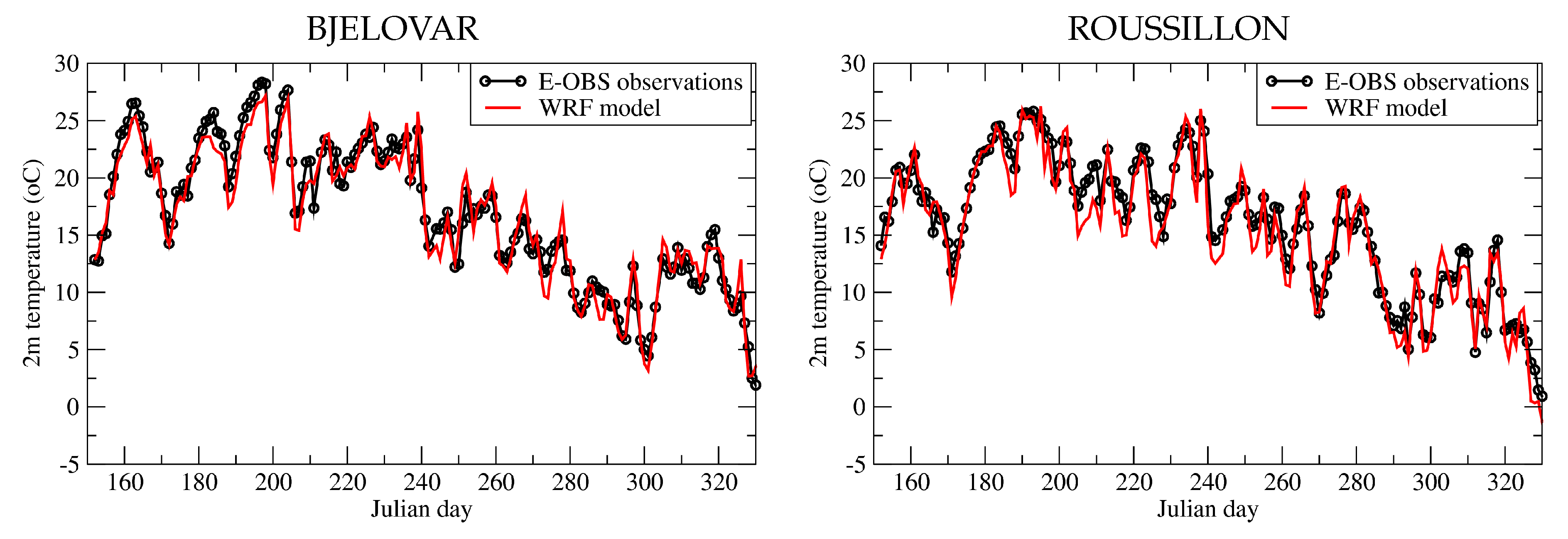
3.2. Comparison between Observed and Modelled 2 m Temperature

Even when we have to use modelled meteorological variables to access all required parameters for release estimates, it is important to quantify if the use of the model will induce a bias in our results or not. One of the most important parameters for ragweed pollen daily release is the 2 m temperature. Fortunately, this variable is available over Europe with observations in the framework of the E-OBS database [49,50]. These only use raw station land data collected from about 3688 meteorological stations throughout Europe and the Mediterranean processed through a series of quality tests to remove errors and unrealistic values. A map of the network is presented in ref. [41]. The three-step interpolation methodology is adapted to ensure that the daily data across the region is homogeneous. In the first step, the monthly mean is interpolated using three-dimensional thin-plate splines to define the spatial trend in the data. The next step is the kriging (minimizing the variance) of the monthly mean anomalies and, finally, applying the anomaly to the interpolated monthly mean to the daily estimate for the final result. The dataset provides the best estimate of the grid box average rather than point value. We, thus, compare time series for this variable and for the locations of the pollen counts measurements. The Pearson’s product moment correlation coefficient, R, is calculated as:

$$R=\frac{{\sum }_{i=1}^n\left(x_i-\overline{x}\right)\left(y_i-\overline{y}\right)}{\sqrt{{\sum }_{i=1}^n{\left(x_i-\overline{x}\right)}^2}\sqrt{{\sum }_{i=1}^n{\left(y_i-\overline{y}\right)}^2}}$$

(1)

This Pearson correlation coefficient is the ratio of the covariance between two data sets x and y and the product of their two standard deviations. A value of 1 is a complete positive correlation. Similarly, a value of −1 represents a complete negative correlation. An important additional piece of information is the significance of this correlation. It is estimated following the Student’s law probability ${\mathrm{p}}_{sl}$. The closer ${\mathrm{p}}_{sl}$ is to zero, the more significant the correlation.

Comparisons between measured and modelled 2 m temperature (in °C) are presented in

Table 4. Comparison between the 2 m temperature representing observations with the E-OBS database and the WRF model. Calculations are done for the stations of pollen counts retained for the study and for the whole year 2010 and using daily mean values. R is the Pearson correlation.

Site	Mean T${}_{2\mathit{m}}$		R	RMSE	Bias
	Model	Obs
BJELOVAR	17.295	17.053	0.969	1.621	0.121
HRZAGR	18.330	16.848	0.969	2.236	0.741
HUDEBR	12.098	10.823	0.966	2.097	0.637
HUGYOE	17.076	16.345	0.967	1.823	0.365
IVANIC	17.346	17.059	0.964	1.740	0.143
ROUSSILLON	14.926	15.095	0.968	1.475	−0.085
SAMOBOR	16.636	16.175	0.965	1.746	0.231
SLAVONSKI	17.960	16.893	0.973	1.884	0.534
VELIKA	17.323	17.505	0.966	1.682	−0.091

. The comparison period is the whole year 2010, and the results show a very high correlation with values always higher than 0.97. In addition, the mean bias is lower than 1 °C. This clearly shows that the use of modelled meteorological variables is completely adapted to the calculation of daily pollen release variability, as presented in this study.

In order to better understand the differences between observations and model, and to discuss the daily variability of the 2 m temperature, Figure 1 presents two time series, corresponding to the sites of BJELOVAR and ROUSSILLON. To better see the temperature values and daily variability, the time series are zoomed over the studied pollen period, from the 1st of June to the 30th of November. This example is for the year 2010. As the two sites are far from each other, the time series show different daily values and variability. However, in the two cases, the two modelled time series are very close to the observations. Clearly, the modelling of this variable is correct and, thus, is not the main reason if the pollen emissions are not realistic enough.

3.3. Statistics between Ragweed Pollen Concentrations and Meteorological Variables at Daily Time Scale

In order to calculate the correlation between the meteorological datasets, the parameterised release term and the observed pollen counts, the Pearson’s product moment correlation coefficient, R, is used. An important additional piece of information is the significance of this correlation. It is estimated following the Student’s law probability ${\mathrm{p}}_{sl}$. The closer ${\mathrm{p}}_{sl}$ is to zero, the more significant the correlation.

Following previous studies, some meteorological variables are of particular importance for pollen emissions. For birch pollen, ref. [16] showed that the most important parameter to take into account is the friction velocity. The surface temperature and relative humidity, as well as the wind speed, act as resistances to this emission flux. Sofiev et al. [20] used the temperature heat-sum function to estimate the starting season, and the flux is moderated by meteorological factors, such as the wind speed, the relative humidity, and the precipitation rate.

Since the ragweed emission process is different from that of birch, we increase the number of potentially correlated parameters. In order to take into account the specific plant phenology, its height above the ground, its sensitivity to temperature and humidity, the examined meteorological variables are listed in Table 3. For each parameter, the temporal averaging is also reported. Note that the ragweed plant being close to the ground, the 10 m wind speed is not taken into account, the near-surface dynamical processes being better represented by the friction velocity, $u_{*}$. The wind direction is not taken into account: even if this variable is important at a very local scale [29,51], it is not the case with our low horizontal resolution: we consider here that the emission is a column process and the wind direction is used in the model only for the horizontal transport. Results are presented in

Table 5. Correlation, R, and significance, ${\mathrm{p}}_{sl}$, between ragweed pollen concentrations and meteorological variables for four stations: ROUSSILLON, HUDEBR, HRZAGR and VELIKA and the year 2010. The definition of the variables and their units are explained in Table 3.

Station	${\mathit{d}}_{\mathbf{mean}}$	${\mathit{d}}_{\mathbf{max}}$	${\mathit{d}}_{\mathbf{morn}}$	${\mathbf{\Delta }}_{\mathbf{morn}}$
ROUSSILLON
	R (p${}_{sl}$)	R (p${}_{sl}$)	R (p${}_{sl}$)	R (p${}_{sl}$)
$T_{2m}$	0.66 (0.00)	0.63 (0.00)	0.65 (0.00)	0.18 (0.18)
$q_{2m}$	0.40 (0.00)	0.40 (0.00)	0.32 (0.01)	−0.11 (0.41)
$u_{*}$	0.11 (0.42)	0.11 (0.39)	0.10 (0.47)	−0.14 (0.29)
$w_{*}$	0.17 (0.22)	0.37 (0.00)	0.22 (0.09)	0.00 (1.00)
$Pr$	−0.05 (0.72)	0.00 (0.99)	−0.10 (0.47)	−0.08 (0.54)
$BLH$	0.33 (0.01)	0.51 (0.00)	0.37 (0.00)	0.45 (0.00)
$Q_0$	−0.03 (0.82)	0.11 (0.43)	0.05 (0.72)	0.18 (0.19)
$S{W}_d$	0.12 (0.36)	0.18 (0.17)	0.18 (0.18)	0.17 (0.20)
HUDEBR
	R (p${}_{sl}$)	R (p${}_{sl}$)	R (p${}_{sl}$)	R (p${}_{sl}$)
$T_{2m}$	0.41 (0.00)	0.42 (0.00)	0.44 (0.00)	−0.13 (0.27)
$q_{2m}$	0.32 (0.01)	0.37 (0.00)	0.33 (0.00)	0.24 (0.04)
$u_{*}$	−0.26 (0.02)	−0.16 (0.18)	−0.18 (0.12)	−0.06 (0.59)
$w_{*}$	0.04 (0.74)	0.15 (0.20)	0.15 (0.19)	0.00 (1.00)
$Pr$	0.13 (0.25)	0.21 (0.07)	0.24 (0.04)	0.38 (0.00)
$BLH$	−0.03 (0.79)	0.20 (0.09)	0.23 (0.05)	0.24 (0.04)
$Q_0$	−0.01 (0.93)	0.02 (0.85)	0.05 (0.69)	−0.20 (0.09)
$S{W}_d$	0.37 (0.00)	0.38 (0.00)	0.37 (0.00)	−0.07 (0.55)
HRZAGR
	R (p${}_{sl}$)	R (p${}_{sl}$)	R (p${}_{sl}$)	R (p${}_{sl}$)
$T_{2m}$	0.22 (0.13)	0.35 (0.01)	0.29 (0.05)	0.19 (0.19)
$q_{2m}$	−0.08 (0.58)	−0.05 (0.71)	−0.06 (0.68)	−0.22 (0.14)
$u_{*}$	−0.23 (0.12)	−0.18 (0.21)	−0.10 (0.50)	0.01 (0.95)
$w_{*}$	0.24 (0.09)	0.27 (0.06)	0.31 (0.03)	0.00 (1.00)
$Pr$	−0.07 (0.65)	−0.08 (0.60)	−0.09 (0.55)	−0.09 (0.53)
$BLH$	−0.09 (0.53)	0.11 (0.45)	0.11 (0.44)	0.07 (0.64)
$Q_0$	0.44 (0.00)	0.42 (0.00)	0.40 (0.01)	0.20 (0.16)
$S{W}_d$	0.28 (0.05)	0.30 (0.04)	0.29 (0.05)	0.11 (0.46)
VELIKA
	R (${\mathrm{p}}_{sl}$)	R (${\mathrm{p}}_{sl}$)	R (${\mathrm{p}}_{sl}$)	R (${\mathrm{p}}_{sl}$)
$T_{2m}$	0.35 (0.01)	0.32 (0.02)	0.33 (0.02)	−0.02 (0.92)
$q_{2m}$	0.32 (0.02)	0.35 (0.01)	0.23 (0.10)	−0.16 (0.28)
$u_{*}$	−0.06 (0.68)	−0.04 (0.78)	0.06 (0.68)	−0.12 (0.39)
$w_{*}$	0.34 (0.01)	0.38 (0.01)	0.43 (0.00)	0.00 (1.00)
$Pr$	−0.06 (0.70)	0.04 (0.78)	−0.03 (0.81)	0.40 (0.00)
$BLH$	0.15 (0.31)	0.27 (0.06)	0.35 (0.01)	0.18 (0.22)
$Q_0$	0.44 (0.00)	0.43 (0.00)	0.44 (0.00)	0.23 (0.10)
$S{W}_d$	0.34 (0.02)	0.34 (0.02)	0.36 (0.01)	0.11 (0.45)

for the selected sites and for the year 2010. The largest two correlations are boldfaced. The results are dispersed and there is no meteorological parameter with a systematically high correlation value.

The highest correlations are for the 2 m temperature, with values ranging between 0.3 and 0.66. While experimental studies have shown that ragweed pollen emissions are more intense during the morning and thus depend on the morning temperature gradient, this does not clearly appear in our results. Recent studies have also shown that $S{W}_d$ is an important factor for ragweed pollen emissions. This was diagnosed under the form of the day length, and thus, the magnitude of daily received $S{W}_d$, as presented in refs. [1,5], for example. This can be seen from our correlations, with values up to 0.38 for the daily mean ($d_{mean}$) or the daily maximum ($d_{max}$). Furthermore, fair correlation values are found for $w_{*}$. This shows that the emissions are sensitive to the near-surface turbulent heat fluxes. For the four sites, the correlations range from 0.04 to 0.43, with mostly significant values.

Surprisingly, the correlations between concentrations and $P_r$ and $q_{2m}$ are not systematically negative. For example, for ROUSSILLON and HUDEBR, the correlation is positive for $q_{2m}$. Here we used the specific humidity in place of the relative humidity, and this could be the reason. The specific humidity is selected here to represent the water vapour amount but also to be an independent variable from temperature. Finally, the highest correlations are found for thermal and radiative parameters, $T_{2m}$ and $S{W}_d$, rather than dynamical parameters. The choice of a "time window" (e.g., daily mean or daily max) is not significant, except the morning for which the correlations are very low and not significant.

4. Modelling Ragweed Pollen Emission

In order to test the impact of a new emissions release term, we implemented three schemes into the CHIMERE chemistry-transport model. First, we implemented existing schemes already used in other models: (1) P2013: the scheme implemented in the SILAM model as it follows the work of refs. [20,22], (2) E2011: the scheme developed by [21], a modified version of ref. [16]. TS2021 (TS for this study): The third scheme corresponds to the [21] scheme but with an alternative release function. For all emissions schemes, the flux (grains m${}^{-2}$ s${}^{-1}$) may be expressed as:

$$E(x,y,t)=D(x,y)\times P(x,y,t)\times \varphi (x,y,t)\times R(x,y,t)$$

(2)

where $D(x,y)$ is the ragweed density distribution in a number of individual plants per square meter. $P(x,y,t)$ is the annual production of grains per individual plant. $\varphi (x,y,t)$ is the phenology factor in s${}^{-1}$, considering its yearly integrated value is unity. This factor represents the knowledge of the start and end date of the pollen season as well as the shape of these potential emissions. $R(x,y,t)$ is the daily or sub-daily weather-dependent release of pollen grains in the atmosphere, which depends on the hourly (or daily) meteorological variables. $R(x,y,t)$ is unitless. These different terms correspond to two different temporal scales: $D(x,y)$, $P(x,y,t)$ and $\varphi (x,y,t)$ represent “annual” information, where $R(x,y,t)$ represents the “short-term” information for which we want to evaluate the correlation with the meteorological variables. In this work, we focus on the calculation of the $R(x,y,t)$ release factor.

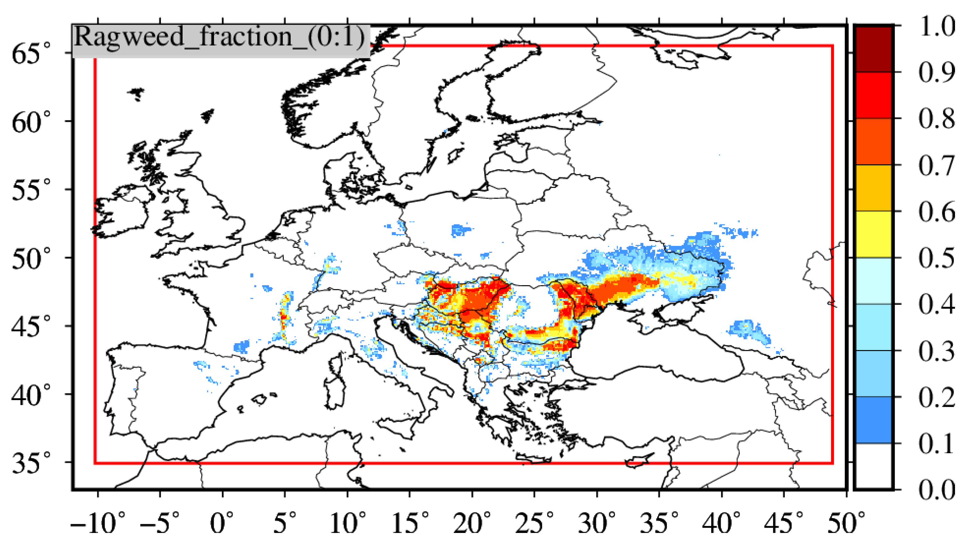
4.1. The Ragweed Plant Fraction in Europe

For the three studied schemes, the terms $D(x,y)$ and $P(x,y,t)$ are the same. They are combined and available through the work of the CAMS pollen forecast group [24]. The distribution of ragweed plants in Europe for the year 2010 is mapped. It is difficult to validate this map having no direct satellite information and the map itself is built using in-situ observations. However, since the goal of this study is to inter-compare emission schemes, and since the same map is used for the three schemes, its uncertainty will not impact the results. Note that new methods are under development and use, mixing in-situ measurements and satellite information on crops, as in ref. [6]. The map used for this study is displayed in Figure 2, where the value indicates the surface fraction occupied by the ragweed plant in a grid cell of resolution 1 × 1 km.

4.2. The Emissions Scheme

The emissions scheme of ref. [22] is used in the paper, referred to as P2013 hereafter. It is the scheme of the SILAM model [20]. Originally developed for birch pollen, it was adapted to ragweed by ref. [22]. This SILAM version is directly implemented in CHIMERE and used without any changes. The goal of this paragraph is not to present this scheme again, which has been extensively described in these two publications. Only the main characteristics and differences with the other schemes are presented. Following P2013, the ragweed pollen emission flux is calculated as:

$$\begin{array}{ccc}\hfill E(i,j,t)& =& N_{tot}\times \varphi (i,j)\times \frac{T-T_{co}}{\Delta H}\times f_{wind}(U,w^{*})\hfill \\ & & \times F_{in}\left(\frac{HS}{H_{start}}\right)\times F_{out}\left(\frac{R\left(t\right)}{N_{tot}}\right)\hfill \\ & & \times f_{thr}(q,q_{low},q_{high})\times f_{thr}(P,P_{low},P_{high})\hfill \end{array}$$

(3)

where $N_{tot}$ is the total number of pollen grains released from 1 m${}^2$ during the whole season, $\varphi (i,j)$ is the plant fraction in grid cell $(i,j)$, $\frac{T-T_{co}}{\Delta H}$ is a relative emission intensity as a linear function of temperature. H is the mean height of the plant. For ragweed, H = 1 m. $F_{in}$ is the emission flux fraction depending on the relative heat sum. $F_{out}$ is the emission flux fraction depending on pollen quantity emitted since the start of the flowering season. $f_{wind}$ is the wind-dependent correction. $f_{thr}$ are the coefficients modulating emissions by humidity and precipitation (between 0 and 1), as:

$$f_{thr}=\left\{\begin{array}{cc}1\hfill & \hfill \mathrm{if}x⩽x_{low}\\ {\displaystyle \frac{x_{high}-x}{x_{high}-x_{low}}}\hfill & \hfill \mathrm{if}{x}_{low}<x<<x_{high}\\ 0\hfill & \hfill \mathrm{if}x⩾x_{high}\end{array}\right.$$

(4)

For the relative humidity, $q_{low}=50\%$ and $q_{high}=80\%$. For the precipitation, $P_{low}=0$, $P_{high}$ = 0.5 mm h${}^{-1}$. Wind speed U and convective turbulence $w^{*}$ impacts are described as:

$$f_{wind}=f_{stagnant}+f_{promote}\left[1.-exp\left(-\frac{w_{10m}+w_{*}}{U_{satur}}\right)\right]$$

(5)

with $w_{10m}$ the 10 m wind speed (m s${}^{-1}$) and w${}^{*}$, the convective velocity scale (m s${}^{-1}$). $f_{stagnant}$ = 0.5, $f_{promote}$ = 1 and $U_{satur}$ = 5 m s${}^{-1}$. The gradual start of the flowering of the plants in a grid cell is described by the relative heat sum $x=\frac{HS\left(t\right)}{H_{start}}$, with the corresponding term $F_{in}\left(x\right)$ given by:

$$F_{in}\left(x\right)=\left\{\begin{array}{cc}0\hfill & \mathrm{if},x<1-\delta \hfill \\ \frac{x-1+\delta }{2\delta }\hfill & \mathrm{if},1-\delta <x<1+\delta \hfill \\ 1\hfill & \mathrm{if},x>1+\delta \hfill \end{array}\right.$$

where $\delta$ = 0.2 is a relative uncertainty of $H_{start}$. The parameter controlling the gradual flowering season termination is the number of grains remaining in catkins with respect to the initial total number of grains $N_{tot}$: $x=\frac{R\left(t\right)}{N_{tot}}$. In the current model version, $N_{tot}$ is prescribed with $N_{tot}={10}^7$ grains per year. An additional map containing a factor is delivered each year in the framework of the CAMS project to recalibrate $N_{tot}$. The corresponding term $F_{out}\left(x\right)$ is given by:

$$F_{out}\left(x\right)=\left\{\begin{array}{cc}1\hfill & \mathrm{if},x<1-\delta \hfill \\ \frac{x+1-\delta }{2\delta }\hfill & \mathrm{if},1-\delta <x<1+\delta \hfill \\ 0\hfill & \mathrm{if},x>1+\delta \hfill \end{array}\right.$$

where $\delta$ = 0.2 is a relative uncertainty of $N_{tot}$.

The heat sum, HS, concept follows the concept of ref. [4], based on biological days. Some input information is necessary to update HS at each model time-step: the current 2 m temperature, the current day, its length in hours and the time step. The HS is updated only if the current day is after the first day, in our case, it is always equal to 79 (i.e., the 20 March). Two ramp functions are estimated, one depending on the 2 m temperature, the second one on the day length. The HS is then equal to:

$$HS=HS+r_T\times l_h\times \frac{\Delta T}{86400}$$

(6)

with:

$$r_t=\left\{\begin{array}{cc}{\displaystyle \frac{T-loTemp}{optTemp-loTemp}}\hfill & \hfill \mathrm{if}loTemp<T<optTemp\\ {\displaystyle \frac{hiTemp-T}{hiTemp-optTemp}}\hfill & \hfill \mathrm{if}optTemp<T<hiTemp\end{array}\right.$$

(7)

the $l_h$ variable is equal to 1 except if the day length ($d_l$) is greater than the photo period parameter, here 14.5 and for the following values:

$$l_h=\left\{\begin{array}{cc}exp((d_l-photoperiod)\times log\left(0.95\right))\hfill & \hfill \mathrm{if}11.5<HS<16\\ exp((d_l-photoperiod)\times log\left(0.94\right))\hfill & \hfill \mathrm{if}16<HS<20.5\end{array}\right.$$

(8)

where the threshold temperature values are fixed. Note that this HS may be reset to zero depending on specific meteorological conditions as:

• T${}_{2m}<$ TempThr (here TempThr = 273.15 K).
• daily mean T${}_{2m}<$ DayTempThr (here DayTempThr = 280.65 K). Note that in this model version, the daily mean 2 m temperature is the running average for the last 24 h.
• HS is lower than StartHSThr. This value is fixed here to StartHSThr = 25.0.

With this scheme, there are no emissions during the night. The calculation of sunrise and sunset is necessary.

4.3. The Emissions Scheme

The approach of ref. [21], herefater called E2011, is a mix between the schemes of [16,19], adapting these formulations to ragweed. In the following, the specific notations of the publications are used to have a reference. The terminology is different from P2013 and [16], but the principle is the same. The pollen emission flux, E (grain m${}^{-2}$ s${}^{-1}$), is calculated as:

$$E=c_e\times c^{*}\times K_e\times u_{*}$$

(9)

The flux depending on the surface grid cell and time, $E(x,y,t)$. The terms of the equation are: $c_e$ a plant specific factor, $c^{*}$ is the grain production factor. The release factor $R_e$ is represented by ($K_e\times u_{*}$). $K_e$ is a time-varying factor depending on weather and $u_{*}$ is the friction velocity. The plant specific factor, $c_e$, is calculated as:

$$c_e=4c_b\left(\frac{d}{S}-\frac{d^2}{S^2}\right)$$

(10)

where $c_b$ is approximated to 10${}^{-4}$. S is the pollen season duration in days, with S = 60. d is the Julian day, varying during the simulation. In practice, the starting and ending dates of the ragweed period are fixed here to 210 and 270 Julian days, respectively. Compared to the values for 2010 in Table 2, this period is slightly larger to enable very low emissions at the start and end of the period. The grain production factor $c^{*}$ is calculated as:

$$c^{*}=\frac{q_p}{LAI\times h_c}$$

(11)

where $q_p$ is the total production of grains per year and is 10${}^9$ grains m${}^{-2}$. It corresponds to the maximum number of emitted grains. Day after day, $q_p$ is reduced by the amount of the already emitted grains the day before. LAI is the leaf area index. LAI is a map in E2011, but in this study, we are using the value of LAI = 3. $h_c$ = 1 m is the canopy height. The $K_e$ variable is estimated as:

$$K_e=K_h\times K_w\times K_r$$

(12)

with the three meteorological limiting factors: $K_h$ for humidity, $K_w$ for 10 m wind speed and $K_r$ for precipitation. For relative humidity, the limiting factor is expressed as Equation (4) with $q_{low}$ = 50% and $q_{high}$ = 80%. For precipitation, we use the fit in E2011 as:

$$K_r=1.-\frac{p}{0.5}$$

(13)

with p the precipitation rate in mm h${}^{-1}$. For the wind speed, $K_w$ is based on P2013 wind correction previously described with Equation (5).

4.4. This Study

The emissions scheme of this study, herefater called TS2021, has the same formulation as the E2011 scheme, except that the release term is reformulated. This release term formulation is inspired by the previously calculated statistical scores but has no direct link to the correlations values. The emissions flux is expressed as:

$$E=c_e\times c^{*}\times R_{TS}$$

(14)

where $c_e$ and $c^{*}$ are the same functions as in the E2011 scheme. $R_{TS}$ (with TS for “this study”) is the new instantaneous release factor. Based on the correlation results of Section 3.3, it appears that the main driving factors are those related to thermodynamical processes, namely the 2 m temperature, $T_{2m}$, vertical velocity scale w${}_{*}$ and shortwave radiation $S{W}_d$. The pollen emissions may be moderated by precipitation rates $P_r$ and 2 m specific humidity $q_{2m}$.

The differences between birch and ragweed emissions could be explained by the plant typology itself: birch is a tree, with the pollen source up to 10 m above the ground. At this level, the wind may be considered as a dominant process for the emission of grains. Ragweed rarely exceeds 1 to 2 m above the ground, where the wind speed is moderate. In this case, the dominant factor could be the temperature, considering the grains are emitted under the highest temperature when they are sufficiently dry [11]. The precipitation rate is a limiting factor but not the most important one: even if it rains during the night, the grains can dry out and can be pulled off the plant in the morning. $R_{TS}$ is thus estimated as:

$$R_{TS}=\frac{{\displaystyle \frac{T_{2m}}{T_{2m,0}}\times \frac{w_{*}}{w_{*,0}}\times \frac{S{W}_d}{S{W}_{d,0}}}}{r_{q_{2m}}+r_{Pr}}$$

(15)

where the values of $T_{2m}$, w${}_{*}$ and $S{W}_d$ correspond to the mean daily value. These values are normalised in order to keep the release term nondimensional. The normalization factors are $T_{2m,0}$ = 10 °C, $w_{*,0}$ = 1 m s${}^{-1}$ and $S{W}_{d,0}$ = 200 W m${}^{-2}$.

In order to moderate these fluxes when meteorological conditions are not favourable, resistance terms are added. These resistances are mainly due to the 2 m specific humidity $q_{2m}$ and the precipitation rate $Pr$. Each resistance is expressed as a sigmoid function ranging between 0 and 1, depending on minimal and maximal value of the x parameter. The resistance has to reflect the fact that these parameters inhibit ragweed pollen emissions.

$$r_x=1+exp\left[\frac{-b_f(i_{max}-i_{min})}{2}\left(\frac{x}{x_{max}-x_{min}}-1\right)\right]$$

(16)

with $b_f$ being a constant chosen here as $b_f$ = 10, which determines the curve of the sigmoid function. $i_{min}$ and $i_{max}$ represent the range of the sigmoid and are here chosen as $i_{min}$ = 0 and $i_{max}$ = 1 in order to use a normalised function for each resistance. The critical issue here is to choose the minimum and maximum value for each x meteorological parameter. These boundaries have to reflect the best possible range of variations of meteorological variables, for all locations over Europe and for the whole year. The maximum values must be moderate enough in order to provide a realistic resistance: a too low maximum value would give a resistance of 1 too often, while a too high maximum value would give too low resistances. Based on all meteorological values used in this study, the boundaries for the 2 m specific humidity are $q_{2m}\left(min\right)$ = 0 and $q_{2m}\left(max\right)$ = 5 × 10${}^{-3}$ g g${}^{-1}$ and for the precipitation rate are $Pr\left(min\right)$ = 0 and $Pr\left(max\right)$ = 1.5 mm h${}^{-1}$.

5. Results and Discussion

To compare several parameterizations of pollen emissions, a simulation is performed over the whole of Western Europe for the year 2010. This simulation includes the emissions, transport across Western Europe, the mixing and the deposition of ragweed pollen concentrations. The year 2010 was selected because of being the one with the largest number of available data, as listed in Table 1. First, correlations, bias and RMSE between the observed and modelled pollen surface concentrations are calculated for the whole year of 2010. Second, time series are presented. Third, surface concentration maps are compared between the three schemes.

5.1. Statistical Scores

Statistical scores between modelled emissions and observed ragweed pollen concentrations are presented in

Table 6. Statistical scores: correlation R, root mean squared error RMSE and bias, calculated for each station where pollen measurements are available, for the three tested emissions schemes. For the correlation, the best value is in bold.

Site	Obsmean	Modmean	R	RMSE	Bias
P2013: [20]
BJELOVAR	75.76	57.19	0.70	1.76	−18.57
HRZAGR	32.37	17.45	0.73	1.97	−14.92
HUDEBR	130.10	46.01	0.78	0.93	−84.08
HUGYOE	43.28	26.70	0.57	1.04	−16.58
IVANIC	68.60	24.52	0.67	2.25	−44.07
ROUSSILLON	59.89	3.57	−0.08	1.14	−56.32
SAMOBOR	16.24	9.64	0.66	1.66	−6.60
SLAVONSKI	203.47	56.22	0.77	0.94	−147.24
VELIKA	78.93	49.03	0.66	2.65	−29.90
Average	R${}_s$ = 0.71		0.61	1.59	−46.48
E2011: [21]
BJELOVAR	75.76	67.66	0.73	1.46	−8.10
HRZAGR	32.37	20.69	0.81	0.94	−11.68
HUDEBR	130.10	46.90	0.69	0.95	−83.19
HUGYOE	43.28	28.01	0.67	1.25	−15.27
IVANIC	68.60	25.10	0.76	0.80	−43.50
ROUSSILLON	59.89	20.45	0.79	0.76	−39.44
SAMOBOR	16.24	15.03	0.56	2.97	−1.21
SLAVONSKI	203.47	60.53	0.87	0.91	−142.94
VELIKA	78.93	51.69	0.73	2.71	−27.23
Average	R${}_s$ = 0.70		0.73	1.42	−41.40
TS2021: This study
BJELOVAR	75.76	71.50	0.85	1.27	−4.25
HRZAGR	32.37	22.79	0.85	1.05	−9.58
HUDEBR	130.10	51.25	0.77	0.94	−78.85
HUGYOE	43.28	28.30	0.76	0.90	−14.98
IVANIC	68.60	27.08	0.67	0.84	−41.52
ROUSSILLON	59.89	25.23	0.80	0.85	−34.66
SAMOBOR	16.24	16.21	0.52	3.33	−0.03
SLAVONSKI	203.47	72.49	0.80	1.00	−130.98
VELIKA	78.93	55.49	0.56	2.94	−23.44
Average	R${}_s$ = 0.77		0.73	1.46	−37.59

. One correlation value is calculated for each year (i.e., each pollen season) and each site. The same calculations are repeated for the three emission schemes.

The bias is high for the three simulations. It is just because the input amount of pollen grains is probably underestimated for this year and this region. The pollen abundance map used is the same for the three simulations, explaining the same bias. This map is regularly updated in the framework of the CAMS project and a new version would certainly correct this point. However, it is not very important since this study focuses on the day-to-day variability; except for the bias calculation, this kind of underestimation has no impact on the other scores. The root mean squared error is close between the three schemes, station per station. Values are ranging between 0.91 (Slavonski with E2011) and 3.33 (Samobor with TS2021, even if the bias is very low). The most relevant score for this study is the correlation; the best values are obtained for E2011 and this study. For E2011, values are better than TS2021 and P2013 at Slavonski (R = 0.87), Samobor (R = 0.56), Velika (R = 0.73) and Ivanic (R = 0.76). Correlations are better with TS2021 at Roussillon (R = 0.80), Hugyoe (R = 0.76), Bjelovar (R = 0.85) and Hrzagr (R = 0.85). Finally, the spatial correlation is better for TS2021 with R = 0.77, while R = 0.71 for P2013 and R = 0.70 for E2011.

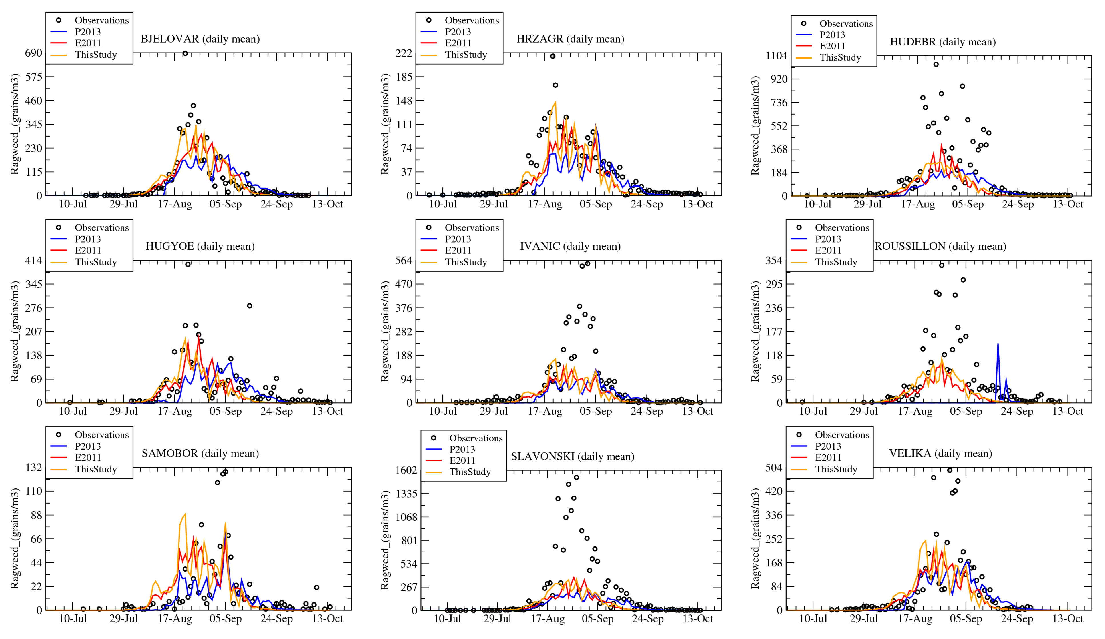
5.2. Time Series of Daily Variabilities

The observed and modelled data used to calculate the statistical scores are displayed in Figure 3. The observations show large temporal variability. Some measurements show very high concentrations, partly explaining the bias (18 August, Bjelovar and Hrzagr, for example). With the model, the day-to-day variability is also high. However, this variability is completely different between the three emission schemes. By comparing E2011 and TS2021, it is surprising to see statistical results relatively close between the two schemes, while the time series are completely different. Globally, even if time series are very variable, the three schemes are able to reproduce the main events of high pollen concentrations for all stations. The only fail is with P2013 at the Roussillon station, when the model starts the emissions too late. This could be explained by an important temperature bias that biases the heat sum. However, the temperature seems to be correctly simulated, as shown in Figure 1. In this case, it is the map of the heat sum threshold, which may be not suitable for the South of France.

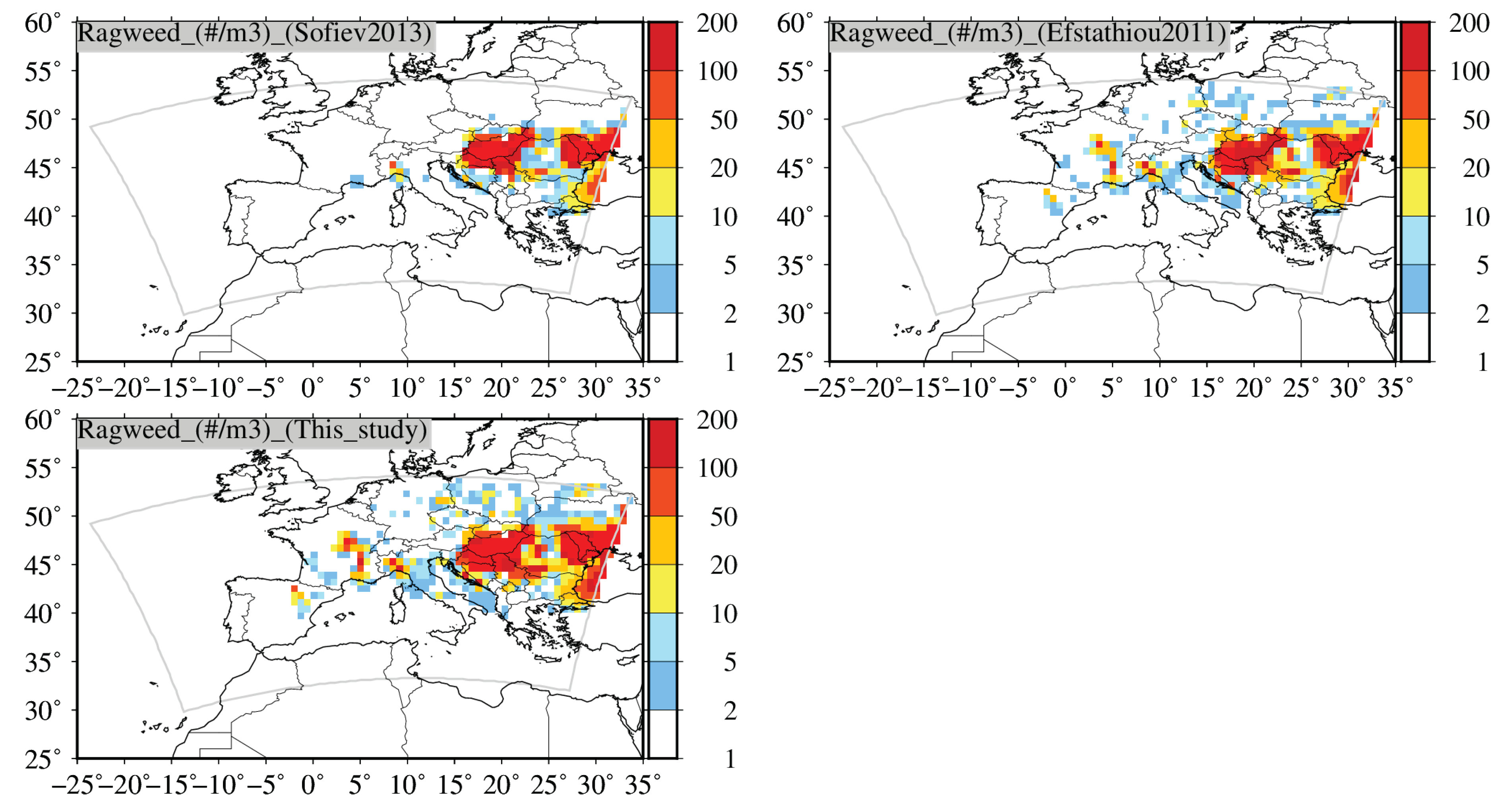
5.3. Surface Concentrations Maps

An example of surface concentrations of ragweed pollen is presented in Figure 4. The maps present values for the 30th August 2010 at 12:00 UTC. Values are represented with a logarithmic colour scale in order to also see the small values. Concentrations are displayed for the first model vertical level, between 0 and 15 m above the surface. The maxima of concentrations are located in the east of Europe, corresponding to the ragweed pollen fraction map presented in Figure 2. The spread is different between the schemes, and P2013 mainly has values in Eastern Europe, but not in the South of France where the Roussillon station is, which explains the low values observed on the time series. E2011 has larger spatial spread than P2013. Lastly, TS2021 has more spatial spread than the two others. The only reason is the day-to-day pollen emission, but not the other processes, since the three configurations are using the same transport and deposition in the model.

6. Conclusions

The modelling of ragweed pollen emissions is sensitive to the daily release term. This release term depends on meteorological parameters. In this study, we propose a new formulation of this term, giving more influence to the near-surface temperature. In order to quantify the impact of several meteorological variables and to sort them compared to pollen grains measurements, statistical scores are calculated. The statistical analysis clearly shows that the highest pollen counts recorded during a season are more sensitive to thermal parameters (2 m temperature) than dynamical variables (wind speed, friction velocity). Using this hierarchy of meteorological variables, a release term is proposed. The statistical analysis being spatially local, the release term is implemented in the CHIMERE chemistry-transport model and compared to two other well-known ragweed pollen emissions schemes [21,22]. A simulation from February to October of 2010 and over Western Europe is performed with the three schemes. The focus of the model analysis is on the capability of the new release term to reproduce the day-to-day variability of emission. Results are compared to the same stations used for the statistical analysis but, this time, including the effects of transport, mixing and deposition. Results show that the new scheme provides better results than the two other schemes, even if differences may be low, specifically when compared to the [21] scheme. However, the latter is more sensitive to mechanical processes, while the new one is more sensitive to thermal surface processes; thus, it is interesting to see that the two schemes give close results.

References

1. Smith, M.; Cecchi, L.; Skjoth, C.; Karrer, G.; Šikoparija, B. Common ragweed: A threat to environmental health in Europe. Environ. Int. 2013, 61, 115–126. [Google Scholar] [CrossRef]
2. Zink, K.; Pauling, A.; Rotach, M.; Vogel, H.; Kaufmann, P.; Clot, B. EMPOL1.0: A new parameterization of pollen emission in numerical weather prediction models. Geosci. Model. Dev. 2013, 6, 1961–1975. [Google Scholar] [CrossRef] [Green Version]
3. Bullock, J.M.; Chapman, D.S.; Schafer, S.; Roy, D.B.; Girardello, M.; Haynes, T.; Beal, S.; Wheeler, B.; Dickie, I.; Phang, Z.; et al. Assessing and Controlling the Spread and the Effects of Common Ragweed in Europe; Technical Report; European Commission Final Report ENV.B.2/ETU/2010/0037; European Commission: Luxembourg, 2012. [Google Scholar]
4. Chapman, D.S.; Haynes, T.; Beal, S.; Essl, F.; Bullock, J.M. Phenology predicts the native and invasive range limits of common ragweed. Glob. Chang. Biol. 2014, 20, 192–202. [Google Scholar] [CrossRef] [Green Version]
5. Thibaudon, M.; Šikoparija, B.; Oliver, G.; Smith, M.; Skjoth, C. Ragweed pollen source inventory for France: The second largest centre of Ambrosia in Europe. Atmos. Environ. 2014, 62–71. [Google Scholar] [CrossRef]
6. Lugonja, P.; Brdar, S.; Simović, I.; Mimić, G.; Palamarchuk, Y.; Sofiev, M.; Šikoparija, B. Integration of in situ and satellite data for top-down mapping of Ambrosia infection level. Remote Sens. Environ. 2019, 235, 111455. [Google Scholar] [CrossRef]
7. Matyasovszky, I.; Makra, L.; Tusnady, G.E.A. Biogeographical drivers of ragweed pollen concentrations in Europe. Theor. Appl. Clim. 2017, 133, 277–295. [Google Scholar] [CrossRef]
8. Schaffner, U.; Steinbach, S.; Sun, Y.; Skjoth, C.A.; de Weger, L.A.; Lommen, S.T.; Augustinus, B.A.; Bonini, M.; Karrer, G.; Šikoparija, B.; et al. Biological weed control to relieve millions from Ambrosia allergies in Europe. Nat. Commun. 2020, 11, 1745. [Google Scholar] [CrossRef] [PubMed] [Green Version]
9. Lake, I.R.; Jones, N.R.; Agnew, M.; Goodess, C.M.; Giorgi, F.; Hamaoui-Laguel, L.; Semenov, M.A.; Solomon, F.; Storkey, J.; Vautard, R.; et al. Climate Change and Future Pollen Allergy in Europe. Environ. Health Perspect. 2017, 125, 385–391. [Google Scholar] [CrossRef]
10. Bianchi, D.; Schwemmin, D.; Wagner, W. Pollen release in the common ragweed (Ambrosia artemisiifolia). Bot. Gaz. 1959, 120, 235–243. [Google Scholar] [CrossRef]
11. Holmes, R.; Bassett, I. Effect of meteorological events on ragweed pollen count. Int. J. Biometeorol. 1963, 7, 27–34. [Google Scholar] [CrossRef]
12. Ogden, E.; Hayes, J.; Raynor, G. Diurnal patterns of pollen emission in Ambrosia, Phleum, Zea and Ricinus. Am. J. Bot. 1969, 56, 16–21. [Google Scholar] [CrossRef] [PubMed]
13. Laaidi, M.; Thibaudon, M.; Besancenot, J.P. Two statistical approaches to forecasting the start and duration of the pollen season of Ambrosia in the area of Lyon (France). Int. J. Biometeorol. 2003, 48, 65–73. [Google Scholar] [CrossRef]
14. Makra, L.; Juhasz, M.; Borsos, E.; Beczi, R. Meteorological variables connected with airborne ragweed pollen in Southern Hungary. Int. J. Biometeorol. 2004, 49, 37–47. [Google Scholar] [CrossRef]
15. Kasprzyk, I. Non-native Ambrosia pollen in the atmosphere of Rzeszow (SE Poland); evaluation of the effect of weather conditions on daily concentrations and starting dates of the pollen season. Int. J. Biometeorol. 2008, 52, 341–351. [Google Scholar] [CrossRef] [PubMed]
16. Helbig, N.; Vogel, B.; Vogel, H.; Fiedler, F. Numerical modelling of pollen dispersion on the regional scale. Aerobiologia 2004, 3, 3–19. [Google Scholar] [CrossRef]
17. Zink, K.; Vogel, H.; Vogel, B.; Magyar, D.; Kottmeir, C. Modeling the dispersion of Ambrosia artemisiifolia L. pollen with the model system COSMO-ART. Int. J. Biometeorol. 2012, 56, 669–680. [Google Scholar] [CrossRef] [PubMed] [Green Version]
18. Makra, L.; Matyasovszky, I.; Tusnády, G.; Wang, Y.; Csépe, Z.; Bozóki, Z.; Nyúl, L.; Erostyák, J.; Bodnar, K.; Sümeghy, Z.; et al. Biogeographical estimates of allergenic pollen transport over regional scales: Common ragweed and Szeged, Hungary as a test case. Agric. For. Meteorol. 2016, 221, 94–110. [Google Scholar] [CrossRef]
19. Sofiev, M.; Siljamo, P.; Ranta, H.; Rantio-Lehtimaki, A. Towards numerical forecasting of long-range air transport of birch pollen: Theoritical considerations and a feasability study. Int. J. Biometeorol. 2006, 50, 392–402. [Google Scholar] [CrossRef]
20. Sofiev, M.; Siljamo, P.; Ranta, H.; Linkosalo, T.; Jeager, S.; Rasmussen, A.; Rantio-Lehtimaki, A.; Severova, E.; Kukkonen, J. A numerical model of birch pollen emission and dispersion in the atmosphere. Description of the emission module. Int. J. Biometeorol. 2013, 57, 45–58. [Google Scholar] [CrossRef] [Green Version]
21. Efstathiou, C.; Isukapalli, S.; Georgopoulos, P. A mechanistic modeling system for estimating large-scale emissions and transport of pollen and co-allergens. Atmos. Environ. 2011, 45, 2260–2276. [Google Scholar] [CrossRef] [Green Version]
22. Prank, M.; Chapman, D.; Bullock, J.; Belmonte, J.; Berger, U.; Dahl, A.; Jager, S.; Kovtunenko, I.; Magyar, D.; Niemela, S.; et al. An operational model for forecasting ragweed pollen release and dispersion in Europe. Agric. For. Meteorol. 2013, 182, 43–53. [Google Scholar] [CrossRef]
23. Liu, L.; Solmon, F.; Vautard, R.; Hamaoui-Laguel, L.; Torma, C.Z.; Giorgi, F. Ragweed pollen production and dispersion modelling within a regional climate system, calibration and application over Europe. Biogeosciences 2016, 13, 2769–2786. [Google Scholar] [CrossRef] [Green Version]
24. Sofiev, M.; Berger, U.; Prank, M.; Vira, J.; Arteta, J.; Belmonte, J.; Bergmann, K.C.; Chéroux, F.; Elbern, H.; Friese, E.; et al. MACC regional multi-model ensemble simulations of birch pollen dispersion in Europe. Atmos. Chem. Phys. 2015, 15, 81158130. [Google Scholar] [CrossRef] [Green Version]
25. Sofiev, M.; Ritenberga, O.; Albertini, R.; Arteta, J.; Belmonte, J.; Bernstein, C.G.; Bonini, M.; Celenk, S.; Damialis, A.; Douros, J.; et al. Multi-model ensemble simulations of olive pollen distribution in Europe in 2014: Current status and outlook. Atmos. Chem. Phys. 2017, 17, 12341–12360. [Google Scholar] [CrossRef] [Green Version]
26. Monks, P.; Granier, C.; Fuzzi, S.; Stohl, A.; Williams, M.; Akimoto, H.; Amann, M.; Baklanov, A.; Baltensperger, U.; Bey, I.; et al. Atmospheric composition change - global and regional air quality. Atmos. Environ. 2009, 43, 5268–5350. [Google Scholar] [CrossRef] [Green Version]
27. Skjøth, C.; Smith, M.; Brandt, J.; Emberlin, J. Are the birch trees in Southern England a source of Betula pollen for North London? Int. J. Biometeorol. 2009, 53, 75–86. [Google Scholar] [CrossRef]
28. Oteros, J.; García-Mozo, H.; Alcázar, P.; Belmonte, J.; Bermejo, D.; Boi, M.; Nanos, P.C.; Díaz de la Guardia, C.; Fernández-González, D.; González-Minero, F.; et al. A new method for determining the sources of airborne particles. J. Environ. Manag. 2015, 155, 212–218. [Google Scholar] [CrossRef] [PubMed]
29. Rojo, J.; Pérez-Badia, R. Spatiotemporal analysis of olive flowering using geostatistical techniques. Sci. Total Environ. 2015, 505, 860–869. [Google Scholar] [CrossRef]
30. Romero-Morte, J.; Rojo, J.; Rivero, R.; Fernández-González, F.; Pérez-Badia, R. Standardised index for measuring atmospheric grass-pollen emission. Sci. Total Environ. 2018, 612, 180–191. [Google Scholar] [CrossRef] [PubMed]
31. Rojo, J.; Orlandi, F.; Pérez-Badia, R.; Aguilera, F.; Ben Dhiab, A.; Bouziane, H.; Díaz de la Guardia, C.; Galán, C.; Gutiérrez-Bustillo, A.M.; Moreno-Grau, S.; et al. Modeling olive pollen intensity in the Mediterranean region through analysis of emission sources. Sci. Total. Environ. 2016, 551–552, 73–82. [Google Scholar] [CrossRef]
32. Oteros, J.; Valencia, R.M.; del Río, S.; Vega, A.M.; García-Mozo, H.; Galán, C.; Gutiérrez, P.; Mandrioli, P.; Fernández-González, D. Concentric Ring Method for generating pollen maps. Quercus as case study. Sci. Total Environ. 2017, 576, 637–645. [Google Scholar] [CrossRef] [PubMed]
33. OECD. Glossary of Statistical Terms; Technical Report; OECD: Paris, France, 2008; ISBN 978-92-64-025561-0. [Google Scholar]
34. WMO. World Meteorological Organization: Guide to Meteorological Instruments and Methods of Measurement; Technical Report; WMO-No. 8; WMO: Geneva, Switzerland, 2008. [Google Scholar]
35. Skjøth, C.; Smith, M.; Šikoparija, B.; Stach, A.; Myszkowska, D.; Kasprzyk, I.; Radisic, P.; Stjepanovic, B.; Hrga, I.; Apatini, D.; et al. A method for producing airborne pollen source inventories: An example of Ambrosia (ragweed) on the Pannonian Plain. Agric. For. Meteorol. 2010, 150, 1203–1210. [Google Scholar] [CrossRef]
36. Hirst, J.M. An automatic volumetric spore trap. Ann. Appl. Biol. 1952, 39, 257–265. [Google Scholar] [CrossRef]
37. Galán, C.; Smith, M.; Thibaudon, M.; Frenguelli, G.; Oteros, J.; Gehrig, R.; Berger, U.; Clot, B.; Brandao, R. Pollen monitoring: Minimum requirements and reproducibility of analysis. Aerobiologia 2014, 30, 385–395. [Google Scholar] [CrossRef]
38. Hamaoui-Laguel, L.; Vautard, R.; Liu, L.; Solmon, F.; Viovy, N.; Khvorostyanov, D.; Essl, F.; Chuine, I.; Colette, A.; Semenov, M.A.; et al. Effects of climate change and seed dispersal on airborne ragweed pollen loads in Europe. Nat. Clim. Chang. 2015, 5, 766–771. [Google Scholar] [CrossRef]
39. Bastl, K.; Kmenta, M.; Berger, U. Defining Pollen Seasons: Background and Recommendations. Curr. Allergy Asthma Rep. 2018, 18, 73. [Google Scholar] [CrossRef] [Green Version]
40. Ziska, L.H.; Makra, L.; Harry, S.K.; Bruffaerts, N.; Hendrickx, M.; Coates, F.; Saarto, A.; Thibaudon, M.; Oliver, G.; Damialis, A.; et al. Temperature-related changes in airborne allergenic pollen abundance and seasonality across the northern hemisphere: A retrospective data analysis. Lancet Planet. Health 2019, 3, e124–e131. [Google Scholar] [CrossRef] [Green Version]
41. Menut, L.; Tripathi, O.; Colette, A.; Vautard, R.; Flaounas, E.; Bessagnet, B. Evaluation of regional climate simulations for air quality modelling purposes. Clim. Dyn. 2013, 40, 2515–2533. [Google Scholar] [CrossRef]
42. Jacob, D.; Petersen, J.; Eggert, B.; Alias, A.; Christensen, O.B.; Bouwer, L.M.; Braun, A.; Colette, A.; Déqué, M.; Georgievski, G.; et al. EURO-CORDEX: New high-resolution climate change projections for European impact research. Reg. Environ. Chang. 2014, 14, 563–578. [Google Scholar] [CrossRef]
43. Vautard, R.; Gobiet, A.; Jacob, D.; Belda, M.; Colette, A.; Deque, M.; Fernandez, J.; Garcia-Diez, M.; Goergen, K.; Guttler, I.; et al. The simulation of European heat waves from an ensemble of regional climate models within the EURO-CORDEX project. Clim. Dyn. 2013, 41, 2555–2575. [Google Scholar] [CrossRef]
44. Hong, S.Y.; Dudhia, J.; Chen, S. A revised approach to ice microphysical processes for the bulk parameterization of clouds and precipitation. Mon. Weather Rev. 2004, 132, 103–120. [Google Scholar] [CrossRef]
45. Mlawer, E.; Taubman, S.; Brown, P.; Iacono, M.; Clough, S. Radiative transfer for inhomogeneous atmospheres: RRTM a validated correlated-k model for the longwave. J. Geophys. Res. 1997, 102, 16663–16682. [Google Scholar] [CrossRef] [Green Version]
46. Chen, F.; Dudhia, J. Coupling an advanced land surface-hydrology model with the Penn State-NCAR MM5 modeling system. Part I: Model implementation and sensitivity. Mon. Weather Rev. 2001, 129, 569–585. [Google Scholar] [CrossRef] [Green Version]
47. Hong, S.Y.; Noh, Y.; Dudhia, J. A new vertical diffusion package with an explicit treatment of entrainment processes. Mon. Weather Rev. 2006, 134, 2318–2341. [Google Scholar] [CrossRef] [Green Version]
48. Grell, G.; Dévényi, D. A generalized approach to parameterizing convection combining ensemble and data assimilation techniques. Geophys. Res. Lett. 2002, 29, 38-1–38-4. [Google Scholar] [CrossRef] [Green Version]
49. Haylock, M.R.; Hofstra, N.; Tank, A.M.G.K.; Klok, E.J.; Jones, P.D.; New, M. A European daily high-resolution gridded data set of surface temperature and precipitation for 1950-2006. J. Geophys. Res. Atmos. 2008, 113, D20119. [Google Scholar] [CrossRef] [Green Version]
50. Cornes, R.C.; van der Schrier, G.; van den Besselaar, E.J.M.; Jones, P.D. An Ensemble Version of the E-OBS Temperature and Precipitation Data Sets. J. Geophys. Res. Atmos. 2018, 123, 9391–9409. [Google Scholar] [CrossRef] [Green Version]
51. Maya-Manzano, J.; Sadyś, M.; Tormo-Molina, R.; Fernández-Rodríguez, S.; Oteros, J.; Silva-Palacios, I.; Gonzalo-Garijo, A. Relationships between airborne pollen grains, wind direction and land cover using GIS and circular statistics. Sci. Total. Environ. 2017, 584–585, 603–613. [Google Scholar] [CrossRef]
Figure 1. Time series of observed (E-OBS) and modelled (WRF) 2 m temperature for the sites of BJELOVAR and ROUSSILLON and for the period ranging from the 1st June to the 30 November 2010.
Atmosphere 12 00693 g001
Figure 2. Distribution of ragweed plants over Europe. Data from the CAMS project [24].
Atmosphere 12 00693 g002
Figure 3. Time series of observed and modelled ragweed pollen surface concentrations for several stations and the year 2010.
Atmosphere 12 00693 g003
Figure 4. Maps of ragweed pollen surface concentrations for the 30 August 2010 at 12:00 UTC for the three studied schemes: P2013 (noted Sofiev2013 on the map), E2011 (noted Efstathiou2011 on the map) and TS2021 (noted This Study, on the map).
Atmosphere 12 00693 g004