Abstract
Forecasting concentration levels is important for planning atmospheric protection strategies. In this paper, we focus on the daily average surface ozone (O) concentration with a short-time resolution (one day ahead) in the Grand Casablanca Region of Morocco. The database includes previous day O concentrations measured at Jahid station and various meteorological explanatory variables for 3 years (2013 to 2015). Taking into account the multicollinearity problem in the data, adapted statistical models based on parametric (SPLS and Lasso) and nonparametric (CART, Bagging, and RF) models were built and compared using the coefficient of determination and the root mean square error. We conclude that the parametric models predict better than nonparametric ones. Finally, from the explanatory variables stored by the SPLS and Lasso parametric models, we deduce that a very simple linear regression with five variables remains the most appropriate for the available data at Jahid station ( = 0.86 and = 9.60). This resulting model, with few explanatory variables to prevent missing data, has good predictive quality and is easily implementable. It is the first to be built to predict ozone pollution in the Grand Casablanca region of Morocco.
1. Introduction
Over the past decades, several studies have been developed, clearly showing the impact of air pollution on human health [1,2], the environment, the natural resources, and the sustainable development of many regions [3]. Morocco is one of the countries with an arid or semi-arid climate, especially those on the southern shore of the Mediterranean, are exposed to air pollution. The barren soils and the high temperature give rise to high O emissions due not only to automobile traffic and industrialization but also to significant soil contributions, linked to the aridity of the climate and the proximity of the desert [4]. Therefore, Morocco is not far from this deterioration of ecological conditions, particularly in large areas where 13.4% of Moroccan population and most the human activities are accumulated (Industries, vehicles, etc.) such as the Grand Casablanca Region (GCR) [5]. O is a secondary trace gas in the atmosphere, and it is not directly emitted from a natural or anthropogenic source but rather formed by a complex set of chemical reactions involving nitrogen oxides (NOx), carbon monoxide (CO), methane (CH), and volatile organic compounds (VOC) in the presence of the sun [3]. Surface O concentrations are also influenced by meteorological conditions that have a significant role in the transport of concentrations of this pollutant such as temperature, pressure, humidity, wind direction, sunshine duration, etc. [4,6,7]. O threatens human health and environment [3,8]. In fact, epidemiological studies have shown that current ambient exposures are associated with reduced basic pulmonary function, exacerbation of asthma, and premature mortality [1,9]. To avoid this problem, the prediction of O concentrations remains a crucial and necessary step in controlling pollution and in mitigating its adverse effects. However, the series of chemical reactions before the emission of ozone into the troposphere during the formation process complicates its forecast [10,11].
In the absence of a statistical forecast model to predict daily ozone from one day to the next for the most critical air pollutants in GCR, the current study is considered the first of its kind in Morocco. The statistical approach is based on historical data in order to predict the future behavior of O associated in large part with meteorological conditions [12]. During the last decade, many researchers have studied the problem of forecasting tropospheric ozone using multivariate statistical methods.These methods can be classified into two main categories: parametric and nonparametric methods [13,14,15]. Recent studies, such as [16,17,18,19,20,21], have compared the performance of these forecasting methods in selecting the most appropriate one. The results have shown that Multiple Linear Regression (MLR), regression tree, and Random Forests give good results. However, these methods are still associated with disadvantages that make interpretation more difficult such as the following: (i) the MLR retains a large number of predictors, which often present multicollinearity problems solved in our last paper by comparing nine alternative regression models [22], and (ii) the construction process of the regression tree and random forests methods remains complex [23]. In addition, these methods require more time during their development and are not recommended when the data history is limited with missing data (case of GCR).
In this regard, the paper at hand proposes a new model that can be easily implemented and provides predictions of O concentrations with a reduced number of explanatory variables that retain good predictive qualities. This model is based on a reduced data history of 3 years (2013, 2014, and 2015) containing missing data. The final model was built and validated by the following process: (i) development of the model in the data from 2013 and 2014 by introducing observed meteorological variables and (ii) validation of the model using data from 2015 by injecting predicted meteorological variables. The results obtained are very satisfactory in terms of the predictive capacity compared to the other models in the present study.
The article at hand is organized as the follow: Section 2 is devoted to the study’s area, the description and analysis of the data, the brief description of the parametric and nonparametric statistical models compared, and the model evaluation. Section 3 sheds light on the results obtained, and Section 4 provides a general discussion with perspectives.
2. Materials and Methods
2.1. Study Area and Data Collection
Morocco is an African country located in the extreme northwest of the continent. It is located in the southern part of the Mediterranean basin and is considered among the most vulnerable countries to climate variability and trans-boundary air pollution [24]. The Grand Casablanca (Figure 1) is the studied region (333442.44 North, 73623.89 West), is located in the central-western part of the Kingdom of Morocco on the Atlantic Ocean coast, and covers an area of 1117 km. The Grand Casablanca Region (GCR) has experienced rapid expansion and increased population growth. It concentrates nearly 13.4% of the total population of the country. Its population is estimated at 4,270,750 residents in 2014 according to World Population Review web-page [5]. In addition, GCR is also one of the most important regions in Africa because it is seen as a hub of economic and business activity. The climate is Mediterranean with a strong oceanic tendency. Temperature can rise up to 40 °C. During the day, the region suffers from mixed episodes (alternating ocean winds, offshore breezes, and synoptic flow) resulting from anticyclonic type conditions that translate into a northeasterly flow [5]. In general, air pollution by the O pollutant depends on several meteorological parameters and the modeling of this phenomenon requires a complete study of the available database. The data over the study area were provided by the General Directorate of Meteorology (GDM) as a result of a scientific cooperation agreement between the GDM and the Poly-disciplinary Faculty of Larache, where this work was conducted. The historical records of these data cover a 3-year period: from 1 January 2013 to 31 December 2015 corresponding to (i) observed meteorological data measured by the meteorological station; (ii) next day’s forecast meteorological data corresponding to the outputs from the numerical meteorological forecast model called “Albachir”, which is based on the community model ALADIN (Limited Area Dynamic Adaptation International Development) [24]; and (iii) O concentrations measured at the Jahid station located in the center of Casablanca City (Figure 1) and having the most important historical record compared to other stations within the region. All statistical analyses were performed using the free software R (http://www.r-project.org (accessed on 1 April 2021)).
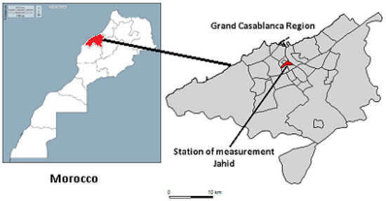
Figure 1.
Map of GCR. The measurement station is a urban station (Jahid) located in the center of Casablanca. Source: Global Administrative Areas (GADM).
2.2. Modelling Approach
The statistical approach adopted in this study is focused on the comparison of two types of forecasting models most frequently used in the literature: parametric (Appendix A) and nonparametric models (Appendix B). In the parametric models, two parsimonious alternative methods to the Multiple Linear Regression (MLR), Sparse Principal Least Squares (SPLS) [25], and Least Absolute Shrinkage and Selection Operator (Lasso) regression [26,27] methods were selected, which conserve a limited number of the most significant variables using penalties on the norm of the variable weights for SPLS and on the L1 norm of the coefficient vector for Lasso. A more detailed description of the two methods can be found in Appendix A.
At the level of nonparametric models, three methods often used in ozone forecasting have been studied: (i) Classification and Binary Regression Tree (CART) [28], which provides a binary regression tree facilitating the identification of the most important variables; (ii) Bootstrap Aggregating (Bagging) [29], which is a random method that allows a user to average the predictions of several independent models by reducing the variance and the prediction error under the boostrapping principle; and (iii) Random Forests (RF) [30], which is an improvement in Bagging that allows a user to aggregate regression trees by inserting a random selection of a limited number of variables among all of the studied predictors variables. The details of these methods are given in Appendix B. Several statistical studies combining previous day’s ozone and meteorological factors to predict daily O concentrations have been published. Various studies in different countries have used a modeling approach based on the following models:
- parametric linear models (Multiple Linear Model and its alternative models): Brazil [31], Canada [32], China [33], Croatia [34], Greece [35], Italy [36], Portugal [14], Spain [37], Malaysia [38], the United States [39], Mexico [21], etc.
- nonparametric models (CART Tree, Bagging, and Random Forests): the United States [40], France [41], Spain [42], China [17], Sweden [43], etc.
In this context, a comparison between these different models was performed in a first step and used the best models obtained in the construction of a new model in a second step. This final regression model was qualified by a reduced number of predictor variables and was easily implementable. It is the first model for daily ozone forecasting in Morocco, more precisely in the GCR.
2.3. Model Evaluation
The evaluation of the fit and performance of the models were performed in two phases necessary to interpret and compare the results of the models, called cross-validation technique. The evaluation of the fit and performance of the models was conducted in two main steps following the cross-validation technique [12,26]. The first phase concerns the internal validation performed on the training data sets, and the second one is called external validation performed on the test data. This is a simple technique that considers the first data set as a training sample (67% of the total data) and the second sample as test or validation data (33% of the total data including observed and predicted meteorological data). The test data set is not used to develop the model but only to evaluate it. Since the present study is based on a 3 year records, the spirit of threefold cross validation has been chosen [44]. The sample is divided into three subsets of one year and for each fold. After that, the models were estimated on all subsets except one (see Figure 2). The left out subset is used to test the model and to determine the most accurate O prediction model in terms of predictive capability.
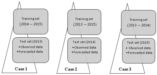
Figure 2.
Scheme of the three cases tested using the spirit of k-fold cross validation technique.
After comparing the obtained results from the models tested for each case of study according to the examined three years (2013–2015), the third case according to the real chronological order was chosen (Figure 2). Indeed, this period is marked by a stability in the results of the studied models, thus ensuring a better forecast. Table A1 and Table A2 give the results obtained in case 1 and case 2, respectively.
During the adjustment (internal validation) and validation (external validation) of the different models on training and test data, the comparison of their performance was evaluated with the main types of statistical criteria and calculated at each step by equations for and .
- The coefficient of determination denoted . This statistic (Equation (1)) provides a measure of the proportion of the variance in the response variable that is predictable from the explanatory variables. It gives some information about the goodness of fit of a model. It is ranges from 0 to 1: the closer its value is to 1 the better the model is.where is the size of training sample, is the y value for i observation, is the mean y value, and is the prediction of i observation obtained using the MLR model (Appendix A).
- The Root Mean Squared Error () is the standard deviation of the residuals (prediction errors). This is computed according to the following expression (Equation (2)):The smallest value of this criterion corresponds to the best goodness of fit of the model.To assess the predictive capacity of the models, we use the RMSE criterion calculated from the observed data of summer 2015 named (Equation (3)):where is the size of the observed the validation set (obstest).Obviously, the best predictive model corresponds to the smallest .In the same way, the of prevision based on the real forecasted meteorological data set on 2015 named is defined as follows (Equation (4)):where is the size of the sample size of the forecasted data (prevtest).
3. Results
In this section, the results obtained with two studied categories of models are presented: parametric (SPLS and Lasso) and nonparametric ones (CART, Bagging, and RF). The purpose of this study is to propose the simplest statistical model for predicting daily O from day i to day taking into account the least number of variables to prevent the problem of missing values.
3.1. Data Preparation
We dispose of 23 quantitative explanatory variables for the observed and forecasted meteorological data set including sunshine duration, temperature, relative humidity, wind speed, wind direction, pressure, etc. as well as the pollution data (ozone concentrations on the days i and ). Table 1 below provides the variable’s abbreviation and units of measurement.

Table 1.
Variable abbreviations and units of measurement.
Historical data related to the three years 2013, 2014, and 2015 were measured in the GCR. Since the aim of our work is to forecast daily O, which is a pollutant qualified as a secondary species and significantly behaves differently depending on the time of the year (summer or winter), the present study was limited to the summer period (April–September) for which ozone concentrations are the highest [7]. Three summer periods were considered (2013, 2014, and 2015), i.e., 549 days. Table 2 presents a description of the observed meteorological and air pollution factors according the different statistical indicators (minimum, maximum, mean, and standard deviation) and the multicollinearity factor . The indicator allows us to analyze the relationship between the predictor variables by using MLR model. The multicollinearity problem is identified as soon as [45]).
Table 2.
Statistics of measured variables at GCR from 01 April to 30 September in 2013 and 2014.
Indeed, the concentration of O during these years is between 10 and 130 µg/m, the maximum temperature (TMPMAX) varies between and 37.50 C, the duration of sunshine (DRINSQ) during the day is between 0 and h, the recorded precipitation (RRQUOT) varies between 0 and mm during the day, atmospheric pressure (PRESTN) during the day at the station is between 998 and 1017 hpa, relative humidity (HUMREL) varies between 0 and 100%, wind speed (FFVM) is null in the morning and up to 7 m/s in the evening, the most dominant wind direction (DDVMDEG) during the day generally comes from the southwest, and horizontal and vertical wind speeds ( and , respectively) are generally low. As the data studied in this paper contain many correlated variables (), nine alternative parametric methods were compared to multiple linear regression (MLR, PCR regression, PLS, SPLS, Continuum Regression, Ridge regression, Lasso, and Biaised Power regression) to resolve the multicollinearity problem [22]. We conclude that the Lasso and SPLS models give the best results. For this reason, we compare them in this paper with the nonparametric methods in order to select the most appropriate one.
The data studied above required a preliminary treatment for the imputation of missing data by the k-nearest neighbor’s method [46] and the agreement between the different meteorological parameters. Multidimensional study on a complete database using a standardized (scaled and centered data) Principal Component Analysis () [47] was conducted. The objective is thus to identify strong correlations between the different predictors to avoid multicollinearity problems [22]. The correlation circle of variables allows us to visualize the different correlations that exist between the meteorological variables and the variable. Therefore, about 40% of the variation is explained by the first two eigenvalues together (Figure 3).
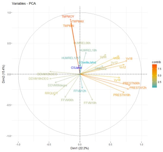
Figure 3.
Correlation circle variables (1−2) factorial plane) according to the contributions of variables to PCs: O3Jahid (dashed blue) considered as a supplementary variable.
We distinguished strong correlations between wind ( and ) and pressure (PRESTN06, PRESTN12, and PRESTN18) parameters on one side and temperature (TMPMAX, TMPMIN, and TMPMOY) on the other. In this respect, using multiple regression model with all of the variables studied is therefore unstable. Indeed, the best adapted model only considers the most significant independent predictors.
3.2. Internal Validation: Goodness of Fit
The goodness of fit of the compared models on the training data (2013 to 2014 period) is assessed by maximizing () criteria and by minimizing the measure. We graphically represent the values of the (Figure 4A) and (Figure 4B) obtained by adjusting the five models over the training period.
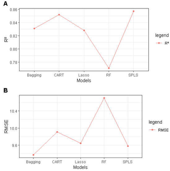
Figure 4.
Comparison of models (A): during summer period of 2013 and 2014; (B): .
Regarding the goodness of fit of the parametric models, the values of obtained by SPLS and Lasso correspond to a good fit ( and , respectively). In the nonparametric models, the CART model shows a good fit of the data (), followed by the Bagging model, which gives results similar to the Lasso model. The non-fixed variables retained by the RF model among the initial twenty-four variables provide an explanatory contribution of 79%, which is still not as good compared to the other models. In addition to the criterion, other performance indices give more precision in terms of the fit quality of models such as the error (Figure 4B) to select the best adjusted model. At first view, the Bagging nonparametric model outperforms the other models by obtaining the lowest value (). The other models are very similar in terms of fit data, recording an error that varies between and , with the exception of the RF model, which has a slightly higher error (). As for the parametric models, SPLS and Lasso register a good fitting in terms of and criteria. However, if the objective is to obtain the best predictive model, the alone is not sufficient to decide on the best forecast model. We therefore use the , calculated on the validation period (2015) during the external validation step, to evaluate the predictive quality of each model.
3.3. External Validation: Performance Evaluation
Model performance is evaluated in this phase with the and calculated from the 2015’s test period, which was not used to adjust the models (Figure 2). Two criteria are calculated:
- , by testing the models on observed meteorological data.
- , by testing the models on the forecasted meteorological data.
Testing the models on observed meteorological data indicates that Lasso and SPLS, respectively, surpass the other methods and remain very similar in terms of predictive capacity. In general, the results obtained from the range from to 14 (Table 3).
Table 3.
A Comparison of the final model with other models according to , , , and criteria.
The most considered results are those of models testing on real forecasted meteorological data. In terms of predictive capacity, it appears that, among the nonparametric models studied, Bagging gives the lowest value of the () followed by its particular case the RF model () and then the Lasso parametric model () (Table 3).
However, for operational purposes, it is preferable to identify a simpler model (with few predictive variables) to avoid the problem of a missing forecast rather than a more complex model with a slightly lower . For this reason, (Figure 5) presents the number of predictive variables retained by each model.
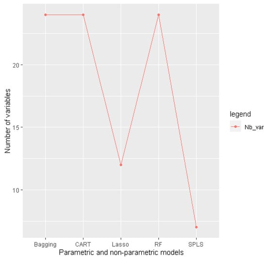
Figure 5.
Comparison of model performance according to number of parameters.
This suggests that Lasso and SPLS retain the advantage of a small number of selected predictive variables (12 and 7, respectively) using the parsimonious principle (reducing the number of predictive variables by applying a penalty that leads to fixing the regression coefficients of the non-selected variables to 0). However, the comparison of the performances of each obtained model using the principle of the threefold cross validation technique (Appendix A and Table A2) reveals that the SPLS and Lasso models appear unstable and more sensitive to the modification of the training and test periods of the data. In this regard, the next section proposes a new simpler multiple regression model with fewer predictor variables ensuring a good prediction quality.
3.4. Selected Forecast Model
The principle of this forecast model is to build a step-by-step regression model from the explanatory variables stored by the SPLS and Lasso parametric models. We thus reduce all explanatory variables of a regression from the first obtained results in Section 3.3. The objective is to obtain a forecasting model that is easier to implement and to interpret in order to obtain short-term forecasts. The regression model that is more important and significantly predictors and high predictive capacity was selected.The scheme below presents the construction process of the selected forecast model (Figure 6).

Figure 6.
Building process of the final forecast model.
Following the adjustment of the new model on the training data set (2013–2014) (internal validation) and its test for the year 2015 (external validation), the results obtained from the different evaluation criteria by comparing them with other models (Section 3.3) are summarized in Table 3.
The selected parametric model for forecast O daily concentrations retains five significant variables: the sunshine duration (), the pressure at 6 h (), the horizontal wind at 6 h (), the vertical wind at 6 h (), and the O concentrations from the previous day (). The model equation is written as Equation (5):
The results of the statistical tests necessary for the diagnosis and validation of the regression model are statistically significant at the 5% significant level. Table A3 summarizes the test’s result.
The regression coefficients obtained from the selected model (Equation (5)) make it possible to explain the impact of the different factors retained on O emissions. Indeed, O concentration is influenced positively by sunshine duration (), horizontal wind direction at 6 h (), and the previous day’s () and negatively by pressure at 6 h () and vertical wind direction at 6 h (). These results are similar to those obtained in studies conducted by [3,21,48].
Table 3 compares the results obtained by the selected reduced regression model with those of the five parametric and non parametric models studied in Section 2.2. This comparison is evaluated using the performance indices of the model’s adjustment quality on learning data ( and ) and prediction quality on test data (2015) ( and ). In terms of adjustment, the selected model provides successful results ( = ) with an of which remains slightly high compared to the SPLS, Lasso, and CART models. In terms of the quality of prediction on observed test data, the final model is very close to that of the Lasso model with ( = ) but remains more accurate than the other models. The validation of the selected model on meteorological forecast data (the summer period of 2015) indicates that it outperforms parametric and nonparametric models in terms of forecasting capacity with the lowest prediction error ( = ). Furthermore, the reduced number of regressors used in the final model (Nb variables = 5) has an important advantage compared to other models, namely, (i) easy prediction of O concentrations and (ii) easy interpretation of the prediction model by avoiding data unavailability.
On this subject, the following graph presents a comparison between the observed O concentration (red color) and the forecasted O concentration (green color) using the selected model with five predictors.
Figure 7 shows that O concentration’s predictions obtained on forecasted meteorological data in 2015 using the selected model are very close to those observed for the same period. This clearly shows the success of the selected regression model in terms of the accuracy of O forecasts for one-step-ahead (i to day) in the GCR. This finally chosen model also provides the best performance on indicators related to forecast quality, such as , , and when compared to the results obtained by Lei [18], which compared the MLR and CART models to forecast O concentrations in Macao.
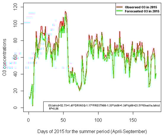
Figure 7.
Comparison between observed and forecasted O concentrations.
4. Discussion
In this study, two statistical approaches were compared to predicting daily ozone in the GCR: (i) parametric models and (ii) nonparametric models. The majority of studies performed to forecast daily ozone have used both parametric and nonparametric statistical models in some way to find a significant relationship between meteorological factors, persistence, and O concentrations [3]. The work conducted in this paper is the first of its kind in Morocco, and the results obtained by similar work performed in other countries were discussed and compared. This comparison remains a complex task that must be carried out with precaution because each country has its own characteristics. In addition, the geographical position, the climate, the history of the data used, and the methodology adopted play very important roles in the development of the forecasting model.
Descriptive statistical analysis of the data; parametric models of the SPLS and Lasso models; and nonparametric models of the CART, Bagging, and RF models were designed to evaluate the best performing model in terms of forecast quality. Several statistical indicators of evaluation were computed, namely , , and (Section 2.3). In terms of the fitting quality, the results of the coefficient of determination obtained by SPLS and Lasso, alternative models to MLR, were satisfactory ( = 0.82, = 0.86) and close to those obtained by the work conducted by [49] (0.6 to 0.90) at different measuring stations, [20] (0.6 to 0.9), [19] (0.60 to 0.80), [50] (0.84). However, Lasso and SPLS appear to be sensitive at the training period level, as they do not maintain their predictive capacity by changing the training period and the test period (Figure 2). Indeed, this instability of the parametric models at the selection level of the complete set of variables is mainly due to the problem of multicollinearity (cf. [22]).
In terms of the nonparametric models, the results obtained for the CART and RF models (0.85 and 0.77, respectively) are similar to those obtained by the author [50] (0.86) who compared the MLR model to the CART model as well as [43] (0.78), who compared MLR and RF. In terms of predictive quality, the studied models have been evaluated by the “RMSEPprev” indicator, which is calculated by using forecasted meteorological data for the validation year (2015). The Bagging and RF models showed good predictive capacity (12.65 and 12.85, respectively) compared to CART (13.83), Lasso (13.02), and SPLS (13.61). These results are still very satisfactory compared to the study conducted in Macao by [18] ( = 24.35), obtained using the CART model. However, Bagging and RF have the disadvantage of being considered “black box” models with many variables that can produce missing forecasts in practice. Indeed, this type of model has complications related to the optimization of the time allocated to the calculation of the parameters necessary for their adjustment as well as to the efficiency of their implementation. As the purpose of the present study is to implement the first short-term ozone prediction model in the GCR, it is difficult to implement a model retaining 24 predictors such as Bagging and RF (24 variables) to routinely predict O concentrations.
Following a profound evaluation of the performance of the parametric and nonparametric models, the final chosen model is based on multivariate regression model using a stepwise method on independent variables retained in Lasso and SPLS models. The final model (Section 3.4) that considers only five of the most significant predictors such as (, , , , and ) was selected. In fact, these meteorological factors are coherent with the results obtained in the literature [3,7,21]. This final selected model has the best predictive ability ( = 12.55) compared to the other models. These results are consistent with the findings of [33], who found that the MLR model is better in terms of prediction than RF. In the same context, ref. [51] also found that MLR outperforms the machine learning models in predicting daily ozone in India. In addition to its predictive quality in terms of accuracy, robustness, and efficiency, the final model provides significant improvements such as (i) being more stability, (ii) having a lower number of predictor variables, (iii) being resistant to missing data and multicollinearity problems, (iv) facilitating implementation and interpretation, and (v) being able to adapt to changing situations (new measurement stations and inclusion of additional data sets). Indeed, the final selected model provides a suitable platform for forecasting, showing a good performance (Figure 7) for a first forecasting model in the GCR.
For future research aiming to improve results in terms of forecasting quality, new data will be added to ensure the stability of the selected model and to extend the forecasting over all cities equipped with measuring stations in Morocco. The model obtained in this study is the most appropriate for predicting the usual O concentrations. The question that arises here would be to determine if this model could predict pollution peaks as well. For this purpose, it is interesting to focus on the predictive quality of extreme values and threshold exceedances of ozone. The aim is thus to create an alert system in case of exceedance of the limits. Another important work will be to study the other atmospheric pollutants such as , NO, and SO in Morocco.
Author Contributions
Conceptualization, H.O.; methodology, H.O. and L.B.; software, H.O. and L.B.; validation, L.B. and A.B.; formal analysis, H.O. and L.B.; investigation, H.O., L.B., A.B., and K.K.; resources, H.O., K.K.; data curation, H.O., K.K.; writing—original draft preparation, H.O.; writing—review and editing, H.O., L.B., A.B., and K.K.; visualization, H.O., L.B., A.B., and K.K.; supervision, L.B. and A.B.; project administration, H.O., L.B., and A.B. All authors have read and agreed to the published version of the manuscript.
Funding
This research received no external funding.
Institutional Review Board Statement
Not applicable.
Informed Consent Statement
Not applicable.
Data Availability Statement
The data used in this article are confidential. They are provided by the General Directorate of Meteorology in Morocco.
Acknowledgments
This research was supported in part by the CNRS project MAiROC. The General Directorate of Meteorology of Morocco is gratefully acknowledged for providing the necessary data to conduct the present study.
Conflicts of Interest
The authors declare no conflict of interest.
Abbreviations
The following abbreviations are used in this manuscript:
| GCR | Grand Casablanca Region |
| GDM | General Directorate of Meteorology |
| ALADIN | Limited Area Dynamic Adaptation International Development |
| GADM | Global Administrative Areas |
| MLR | Multiple Linear Regression |
| SPLS | Sparse Partial Least Square |
| LASSO | Least Absolute Shrinkage and Selection Operator |
| CART | Classification and Regression Tree |
| RF | Random Forest |
| VIF | Variance Inflation Factor |
Appendix A. Parametric Models
Appendix A.1. Multiple Linear Regression Model (MLR Model)
In order to describe the parametric models studied in this paper, it is essential to provide the matrix notation of the multiple linear regression model (MLR model) Equation (A1):
where is a vector (centred dependant variable), is a matrix (matrix of standardized predictors), is a vector of unknow regression coefficients, and is a vector of random errors. The distribution of is assumed to be normal with mean equal to 0 and a variance covariance matrix equal to , where is the identity matrix [35]. Usually, the variables in are centered by subtracting their means and scaled by dividing by their standard deviations. In MLR model, the estimated regression coefficients are defined by
In the case of this study, the expression of Equation (A1) becomes Equation (A2):
where is the concentration in O day i, is the previous day’s O concentration (i.e., persistence), and is the value of meteorological variable j day i. For more information about MLR model using in this case, you can refer to [22].
Appendix A.2. Sparse PLS Regression (SPLS)
The Sparse PLS method described in [25] is a direct adaptation of the classic PLS regression method. It is a parsimonious approach that integrates a selection of variables into the PLS by using penalties on the weight norm to make this selection. PLS regression yields latent components such that , where m is the number of latent components . In SPLS regression, the first weight vector as an optimal solution to Equation (A3):
where , is the -norm of vector and is a scalar which controls the degree of sparsity.
The estimated regression coefficients of are calculated by fixing the coefficients of the non-selected variables to 0 and by obtaining the coefficients of the selected variables with the “standard” PLS regression (see Equation (A4)).
The interest of the SPLS is twofold: on the one hand, it reduces the number of explanatory variables, which allows for an easier interpretation of the model, and on the other hand, it avoids the problem of multicollinearity by using the PLS regression model. Moreover, SPLS is computationally efficient with a tunable sparsity parameter to select the important variables.
Appendix A.3. Lasso Regression
The Least Absolute Shrinkage and Selection Operator, or Lasso [26,27], is another penalized regression where the penalty of ridge regression is replaced by an penalty. This is a subtle change that has important consequences. Indeed, this constraint entails that some of the regression coefficients are shrunk exactly to zero. This means that this regression strategy operates a selection of variables since the unimportant variables are discarded, with their regression coefficients being equal to zero. Formally, the lasso estimator is given as a solution to the following optimization problem designed by Equation (A5):
where .
The parameter controls the degree of sparsity: the smaller this parameter, the larger the number of discarded variables. Contrariwise, if is larger than , then . Lasso regression has the double effect of shrinking the coefficients, allowing us to decrease the variance of the regression coefficients as with Ridge regression and, more importantly, to operate an automatic selection of the variables by cancelling out some coefficients.
Appendix B. Nonparametric Models
The nonparametric models used to predict tropospheric ozone in this study are Regression Tree, Bagging, and Random Forests.
Appendix B.1. Classification and Regression Tree (CART)
Ref. [28] is a nonparametric supervised classification or regression method depending on the nature of the variable to be explained (qualitative or quantitative). It is complementary to the above linear regression method in the regression version. It is a method frequently used in air quality prediction [18,26]. This learning method is based on the implementation of a decision tree as a prediction model. The construction of this tree uses the data set for which the value of the target variable is known and then projects the results to the test data. Since the data studied in our paper are quantitative, we are interested in the regression CART tree.
Binary tree’s construction: CART is a binary recursive partitioning technique consisting of splitting the data into two groups, resulting in a binary tree, in which the terminal nodes represent distinct classes or categories of data. Cutting is carried out according to simple rules on the explanatory variables, determining the optimal rule that allows us to build two populations more differentiated in terms of values of the variable to be explained. It builds a partition visualized using a binary tree [26]. A classic stopping rule is not to cut out nodes that contain less than a certain number of observations. Terminal nodes, which are no longer cut out, are called the sheets of the tree.
The objective of a decision tree is to divide the forecast space into K separate class such as, . In the case of the quantitative response variable , regression tree model can be written as the following Equation (A6):
where is the unknown number of sheets of the tree underlying the method, corresponds to the different classes, and are the coefficients to be estimated by the average in each class of the explained variable.
Pruning: After the first step of building the CART tree, the second step called “pruning” consists in removing a posteriori branches of the tree considered unnecessary to find the best tree-pruned for the maximum tree. The idea is that the maximum tree corresponds to a parsimonious model with a very high variance and a low bias.
The CART method is adapted to the case of many explanatory variables of different types, which allows explicit results to be given with simple decision rules that can be easily interpreted and do not disturb extreme observations (e.g., cases of pollution peaks).
However, one of its inconveniences is that the CART method may not reach the optimal model or it may also present instability in the trees obtained (a light perturbation). Indeed, other methods or practices exist that can provide solutions to this type of problem; the main random aggregation methods of forecasting are namely Bagging and Random Forests.
Appendix B.2. Bagging
Bootstrap Aggregation (or Bagging for short) is a random method firstly introduced by Breiman in [29]. It applies the Bootstrap or Bootstrapping principle [52] to the aggregation of predictors. It allows to average the forecasts of several independent models and to reduce the variance as well as the forecast error. To briefly introduce the Bagging, we consider a model function of and a sample of distribution F. Considering B independent samples noted , a model aggregation forecast is defined below by Equation (A7) in the case where the variable to be explained is quantitative:
The samples so obtained are obviously not independent, but the instability of the trees can make the set completely efficient: each tree has a low bias while its mean is of low variance. The parameters number of trees can be determined in practice by the cross-validation technique [41].
The advantage of this method is the simplicity and facility of adaptation to the implementation of the different modelling methods. However, bagging requires a longer computation time to run the model and the model results are not viewed as a decision tree.
Appendix B.3. Random Forests (RF)
The RF method was presented in [30] and more recently for example in [53]. Its objective is to improve Bagging for binary trees (CART) by introducing “randomization”, which makes it possible to develop the trees in the aggregation more independent by adding chance in the choice of variables used in the model. As its name suggests, a RF consists of aggregating trees of discrimination or regression.
We consider the Learning data set, a collection of predictors per tree, where is a series of B independent and identically distributed random variables. The predictor of random forests is obtained by aggregating this collection of trees. A RF is therefore no more than an aggregation of trees dependent on random variables. For example, bagging trees (building trees on bootstrap samples) defines a random forest. A family of random forests is different from others, particularly in terms of the quality of its performance on many data sets. The term” Random Forests” is derived from the fact that individual predictors are, in this case, explicitly predictors per tree and from the fact that each tree depends on an additional random variable (i.e., in addition to the learning data set ). A random forest is a part of the family of group methods based on a decision tree, which makes it possible to aggregate a collection of random trees. Every “tree” in the “forest” is trained with a different learning data set. Each of these sets is a subsample of the set of learning data, randomly selected using the Bagging method. The importance of each variable for the forecast can therefore be estimated posteriori. It is possible to use variables that do not have a statistical link with the response; their importance in the forecast is reduced by the model [41].
The algorithm principle of the RF method is to add a random draw of m among the p explanatory variables in the application of Bagging to binary decision trees. The number of explanatory variables m can be calculated by default in the case of regression problems using the formula . In practice, the parameters number of trees built B and number of variables m require optimization through the application of a cross-validation technique. In general, the RF method avoids over-learning with better performance than decision trees. The parameters are easy to calibrate but its training remains slower and difficult to interpret.
Appendix C. Comparison Table of Parametric and Nonparametric Models
Appendix C.1. Training Period: (2014 –2015) (Case 1)
Table A1.
Comparison table of parametric and nonparametric models according to the , , , , and criteria.
Table A1.
Comparison table of parametric and nonparametric models according to the , , , , and criteria.
| Models/Criteria | |||||
|---|---|---|---|---|---|
| SPLS | 0.827 | 9.299 | 12.77 | 13.98 | 8 |
| Lasso | 0.801 | 9.233 | 12.77 | 13.63 | 14 |
| CART | 0.803 | 9.909 | 13.69 | 13.81 | 24 |
| Bagging | 0.802 | 8.704 | 13.44 | 14.04 | 24 |
| RF | 0.774 | 9.579 | 16.80 | 17.40 | 24 |
Appendix C.2. Training Period: (2013–2015) (Case 2)
Table A2.
Comparison table of parametric and nonparametric models according to the , , , , and criteria.
Table A2.
Comparison table of parametric and nonparametric models according to the , , , , and criteria.
| Models/Criteria | |||||
|---|---|---|---|---|---|
| SPLS | 0.761 | 11.40 | 9.595 | 8.92 | 6 |
| Lasso | 0.751 | 10.94 | 9.151 | 7.63 | 13 |
| CART | 0.757 | 11.48 | 12.41 | 12.62 | 24 |
| Bagging | 0.734 | 10.30 | 10.39 | 10.19 | 24 |
| RF | 0.701 | 11.78 | 10.21 | 8.40 | 24 |
Appendix D
Table A3.
Tests results for the final forecast model’s diagnostic check.
Table A3.
Tests results for the final forecast model’s diagnostic check.
| Test | p-Value | |
|---|---|---|
| Normality (Shapiro–Wilk normality) | Residuals normality | 0.049 |
| Homoscedasticity (Studentized Breusch–Pagan) | Homoscedasticity | 0.8361 |
| Autocorrelation (D–W Autocorrelation ) | = 0 | 0.314 |
| Linearity (Harvey–Collier ) | Nonlinear relation | 0.004 |
References
- Liu, J.C.; Peng, R.D. Health effect of mixtures of ozone, nitrogen dioxide, and fine particulates in 85 US counties. Air Qual Atmos Health 2018, 11, 311–324. [Google Scholar] [CrossRef]
- Lin, X.; Yuan, Z.; Yang, L.; Luo, H.; Li, W. Impact of extreme meteorological events on ozone 346in the pearl river delta, China. Aerosol Air Qual. Res. 2019. [Google Scholar] [CrossRef]
- Wang, T.; Xue, L.; Brimblecombe, P.; Fat Lam, Y.; Li, L.; Zhang, L. Ozone pollution in China: A review of concentrations, meteorological influences, chemical precursors, and effects. Sci. Total Environ. 2017, 575, 1582–15961. [Google Scholar] [CrossRef] [PubMed]
- Khomsi, K.; Chelhaoui, Y.; Alilou, S.; Souri, R.; Najmi, H.; Souhaili, Z. Concurrent heatwaves and extreme Ozone (O3) episodes: Combined atmospheric patterns and impact on human health. Earth Space Sci. Open Arch. 2020, 16, 2020. [Google Scholar] [CrossRef]
- World Population Prospects United Nations Population Estimates and Projections of Major Urban Agglomerations. (2019 Revision). Available online: https://worldpopulationreview.com/world-cities/casablanca-population (accessed on 15 April 2021).
- Yang, L.; Xie, D.; Yuan, Z.; Huang, Z.; Wu, H.; Han, J.; Liu, L. Quantification of regional ozone pollution characteristics and its temporal evolution: Insights from the identification of the impacts of meteorological conditions and emissions. Atmosphere 2021, 12, 279. [Google Scholar] [CrossRef]
- Fang, C.; Wang, L.; Wang, J. Analysis of the Spatial–Temporal Variation of the Surface Ozone Concentration and Its Associated Meteorological Factors in Changchun. Environments 2019, 6, 46. [Google Scholar] [CrossRef]
- Anenberg, S.C.; Horowitz, L.W.; Tong, D.Q.; West, J.J. An estimate of the global burden of anthropogenic ozone and fine particulate matter on premature human mortality using atmospheric modeling. Environ. Health Perspect. 2010, 118, 1189–1195. [Google Scholar] [CrossRef]
- Green, R.; Broadwin, R.; Malig, B.; Basu, R.; Gold, E.B.; Qi, L.; Sternfeld, B.; Bromberger, J.T.; Greendale, G.A.; Kravitz, H.M.; et al. Long- and short-term exposure to air pollution and inflammatory/hemostatic markers in midlife women. Epidemiology 2016, 27, 211–220. [Google Scholar] [CrossRef]
- Van Eijkeren, J.C.; Freijer, J.I.; Van Bree, L. A model for the effect of health of repeated exposure to ozone. Environ. Model Softw. 2002, 17, 553–562. [Google Scholar]
- Leelossy, Á.; Molnár, F.; Izsák, F.; Havasi, Á.; Lagzi, I.; Mészáros, R. Dispersion modeling of air pollutants in the atmosphere: A review. Cent. Eur. J. Geosci. 2014, 6, 257–278. [Google Scholar] [CrossRef]
- Zhang, J.; Ding, W. Prediction of Air Pollutants Concentration Based on an Extreme Learning Machine: The Case of Hong Kong. Int. J. Environ. Res. Public Health 2017, 14, 114. [Google Scholar] [CrossRef] [PubMed]
- Thompson, M.L.; Reynolds, J.; Cox, L.; Guttorp, P.; Sampson, P.D. A review of statistical methods for the meteorological adjustment of tropospheric ozone. Atmos. Environ. 2001, 35, 617–630. [Google Scholar] [CrossRef]
- Sousa, S.I.V.; Martins, F.G.; Alvim-Ferraz, M.C.M.; Pereira, M.C. Multiple Linear Regression and Artificial Neural Networks Based on Principal Components to Predict Ozone Concentrations. Environ. Modell. Softw. 2007, 22, 97–103. [Google Scholar] [CrossRef]
- Zhang, Y.; Bocquet, M.; Mallet, V.; Seigneur, C.; Baklanov, A. Real-time air quality forecasting, part I: History, techniques, and current status. Atmos. Environ. 2012, 60, 632–655. [Google Scholar] [CrossRef]
- Ben Ishak, A.; Ben Daoud, M.; Trabelsi, A. Ozone Concentration Forecasting Using Statistical Learning Approaches. J. Mater. Environ. Sci. 2017, 8, 4532–4543. [Google Scholar] [CrossRef]
- Zhan, Y.; Luo, Y.; Deng, X.; Grieneisen, M.L.; Zhang, M.; Di, B. Spatiotemporal prediction of daily ambient ozone levels across China using random forest for human exposure assessment. Environ. Pollut. 2018, 233, 464–473. [Google Scholar] [CrossRef] [PubMed]
- Lei, M.T.; Monjardino, J.; Mendes, L.; Gonçalves, D.; Ferreira, F. Macao air quality forecast using statistical methods. Air Qual. Atmos. Health 2019, 12, 1049–1057. [Google Scholar] [CrossRef]
- Jahn, S.; Hertig, E. Statistical modelling of combined ozone-temperature events in Europe. In Proceedings of the EGU General Assembly 2020, Online, 4–8 May 2020. EGU2020-1314. [Google Scholar] [CrossRef]
- Allu, S.K.; Srinivasan, S.; Maddala, R.K.; Reddy, A.; Anupoju, G.R. Seasonal ground level ozone prediction using multiple linear regression (MLR) model. Model. Earth Syst. Environ. 2020, 6, 1981–1989. [Google Scholar] [CrossRef]
- Iglesias-Gonzalez, S.; Huertas-Bolanos, M.E.; Hernandez-Paniagua, I.Y.; Mendoza, A. Explicit Modeling of Meteorological Explanatory Variables in Short-Term Forecasting of Maximum Ozone Concentrations via a Multiple Regression Time Series Framework. Atmosphere 2020, 11, 1304. [Google Scholar] [CrossRef]
- Oufdou, H.; Bellanger, L.; Bergam, A.; El Ghaziri, A.; Khomsi, K.; Qannari, E. Comparison of Different Regularized and Shrinkage Regression Methods to Predict Daily Tropospheric Ozone Concentration in the Grand Casablanca Area. Adv. Pure Math. 2018, 8, 793–812. [Google Scholar] [CrossRef][Green Version]
- Bai, L.; Wang, J.; MaID, X.; Lu, H. Air Pollution Forecasts: An Overview. Int. J. Environ. Res. Public Health 2018, 15, 780. [Google Scholar] [CrossRef] [PubMed]
- World Urbanization Prospects—United Nations Population Estimates and Projections of Major Urban Agglomerations. Available online: https://worldpopulationreview.com/world-cities/casablanca-population (accessed on 15 April 2021).
- Wold, H. Estimation of Principal Components and Related Models by Iterative Least Squares. In Multivariate Analysis; Krishnaiah, P.R., Ed.; Academic Press: New York, NY, USA, 1966; pp. 391–420. [Google Scholar]
- Hastie, T.; Tibshirani, R.; Friedman, J. The Element of Statistical Learning: Data Mining, Inference, and Prediction; Springer: Berlin, Germany, 2009; ISBN 978-0-387-84858-7. [Google Scholar]
- Tibshirani, R. Regression shrinkage and selection via the lasso: A retrospective. J. R. Stat. Soc. Ser. B Stat. Method. 2011, 73, 273–282. [Google Scholar] [CrossRef]
- Breiman, L.; Friedman, J.H.; Olshen, R.A.; Stone, C.J. Classification and Regression Trees; Chapman & Hall: New York, NY, USA, 1984. [Google Scholar]
- Breiman, L. Bagging Predictors. Mach. Learn. 1996, 24, 123–140. [Google Scholar] [CrossRef]
- Breiman, L. Random Forests. Mach. Learn. 2001, 45, 5–32. [Google Scholar] [CrossRef]
- Souza, A.; Aristones, F.; Pavão, H.; Fernandes, W. Development of a Short-Term Ozone Prediction Tool in Campo Grande-MS-Brazil Area Based on Meteorological Variables. Open J. Air Pollut. 2014, 3, 42–51. [Google Scholar] [CrossRef]
- Robeson, S.M.; Steyn, D.G. Evaluation and comparison of statistical forecast models for daily maximum ozone concentrations. Almos. Environ. 1990, 246, 303–312. [Google Scholar] [CrossRef]
- Li, H.; Zhu, Y.; Zhao, Y.; Chen, T.; Jiang, Y.; Shan, Y.; Liu, Y.; Mu, J.; Yin, X.; Wu, D.; et al. Évaluation de la performance des capteurs de qualité de l’air à faible coût dans une station de haute montagne avec des conditions météorologiques complexes. Atmosphere 2020, 11, 212. [Google Scholar] [CrossRef]
- Kovac-Andric, E.; Brana, J.; Gvozdic, V. Impact of Meteorological Factors on Ozone Concentrations Modelled by Time Series Analysis and Multivariate Statistical Methods. EcologicalInformatics 2009, 4, 117–122. [Google Scholar] [CrossRef]
- Chaloulakou, A.; Assimacopoulos, D.; Lekkas, T. Forecasting Daily Maximum Ozone Concentrations in the Athens Basin. Environ. Monit. Assess. 1999, 56, 97–112. [Google Scholar] [CrossRef]
- Di Carlo, P.; Pitari, G.; Mancini, E.; Gentile, S.; Pichelli, E.; Visconti, G. Evolution of Surface Ozone in Central Italy Based on Observations and Statistical Model. J. Geophys. Res. D 2007, 112, 10316. [Google Scholar] [CrossRef]
- Barrero, M.A.; Grimalt, J.O.; Canton, L. Prediction of Daily Ozone Concentration Maxima in the Urban Atmosphere. Chemom. Intell. Lab. Syst. 2006, 80, 67–76. [Google Scholar] [CrossRef]
- Marzuki, I.; Al-Mahfoodh, N.; Samsuri, A.M. Development of Ozone Prediction Model in Urban Area. Int. J. Innov. Technol. Explor. Eng. 2019, 8. [Google Scholar] [CrossRef]
- Scheifinger, H.; Stohl, A.; Kromp-Kolb, H.; Spangl, W. A statistical method for predicting daily maximum ozone concentrations. Gefahrstaffe, Reinhaltung der Luft 1996, 56, 133–137. [Google Scholar]
- Ryan, W.F. Forecasting severe ozone episodes in the Baltimore metropolitan area. Atmos. Environ. 1995, 29, 2387–2399. [Google Scholar] [CrossRef]
- Genuer, R.; Poggi, J.M.; Tuleau, C. Variable selection using random forests. Pattern Recognit. Lett. Elsevier 2010, 31, 2225–2236. [Google Scholar] [CrossRef]
- Gómez-Losada, A.; Asencio-Cortés, G.; Martínez-Álvarez, F.; Riquelme, J.C. A novel approach to forecast urban surface-level ozone considering heterogeneous locations and limited information. Environ. Modell. Softw. 2018, 110, 52–61. [Google Scholar] [CrossRef]
- Stafoggia, M.; Johansson, C.; Glantz, P.; Renzi, M.; Shtein, A.; de Hoogh, K.; Kloog, I.; Davoli, M.; Michelozzi, P.; Bellander, T. A Random Forest Approach to Estimate Daily Particulate Matter, Nitrogen Dioxide, and Ozone at Fine Spatial Resolution in Sweden. Atmosphere 2020, 11, 239. [Google Scholar] [CrossRef]
- Geisser, S. The predictive sample reuse method with applications. J. Am. Statist. Assoc. 1975, 70, 320–328. [Google Scholar] [CrossRef]
- James, G.; Witten, D.; Hastie, T.; Tibshirani, R. An Introduction to Statistical Learning; Springer: New York, NY, USA, 2013. [Google Scholar]
- Beretta, L.; Santaniello, A. Nearest neighbor imputation algorithms: A critical evaluation. BMC Med. Inf. Decis. Mak. 2016, 16, 74. [Google Scholar] [CrossRef]
- Jolliffe, I.T. Principal Component Analysis, 2nd ed.; Springer: New York, NY, USA, 2002. [Google Scholar]
- Alvim-Ferraz, M.C.; Sousa, S.I.; Pereira, M.C.; Martins, F.G. Contribution of anthropogenic pollutants to the increase of tropospheric ozone levels in the Oporto Metropolitan Area, Portugal since the 19th century. Environ. Pollut. 2006, 140, 516–524. [Google Scholar] [CrossRef]
- Bekesiene, S.; Meidute-Kavaliauskiene, I.; Vasiliauskiene, V. Accurate Prediction of Concentration Changes in Ozone as an Air Pollutant by Multiple Linear Regression and Artificial Neural Networks. Mathematics 2021, 9, 356. [Google Scholar] [CrossRef]
- Lei, M.T.; Monjardino, J.; Mendes, L.; Gonçalves, D.; Ferreira, F. Statistical Forecast of Pollution Episodes in Macao during National Holiday and COVID-19. Int. J. Environ. Res. Public Health 2020, 17, 5124. [Google Scholar] [CrossRef] [PubMed]
- Pandya, S.; Ghayvat, H.; Sur, A.; Awais, M.; Kotecha, K.; Saxena, S.; Jassal, N.; Pingale, G. Pollution Weather Prediction System: Smart Outdoor Pollution Monitoring and Prediction for Healthy Breathing and Living. Sensors 2020, 20, 5448. [Google Scholar] [CrossRef] [PubMed]
- Altman, N.; Krzywinski, M. Ensemble methods: Bagging and random forests. Nat. Methods 2017, 14, 933–934. [Google Scholar] [CrossRef]
- Cutler, A.; Cutler, R.; Stevens, J.R. Random Forests. Chapter 5: Ensemble Machine Learning: Methods and Applications; Springer: Berlin/Heidelberg, Germany, 2012. [Google Scholar] [CrossRef]
Publisher’s Note: MDPI stays neutral with regard to jurisdictional claims in published maps and institutional affiliations. |
© 2021 by the authors. Licensee MDPI, Basel, Switzerland. This article is an open access article distributed under the terms and conditions of the Creative Commons Attribution (CC BY) license (https://creativecommons.org/licenses/by/4.0/).