Improving the Retrieval of Cloudy Atmospheric Profiles from Brightness Temperatures Observed with a Ground-Based Microwave Radiometer

Abstract

Atmospheric temperature and humidity retrievals from ground-based microwave remote sensing are useful in a variety of meteorological and environmental applications. Though the influence of clouds is usually considered in current retrieval algorithms, the resulting temperature and humidity estimates are still biased high in overcast conditions compared to radiosonde observations. Therefore, there is a need to improve the quality of retrievals in cloudy conditions. This paper presents an approach to make brightness temperature (TB) correction for cloud influence before the data can be used in the inversion of vertical profiles of atmospheric temperature and humidity. A three-channel method is proposed to make cloud parameter estimation, i.e., of the total 22 channels of the ground-based radiometer, three are adopted to set up a relationship between cloud parameters and brightness temperatures, so that the observations from the three channels can be used to estimate cloud thickness and water content and complete the cloud correction for the rest of the channels used in the retrieval. Based on two years of data from the atmosphere in Beijing, a comparison of the retrievals with radiosonde observations (RAOB) shows: (1) the temperature retrievals from this study have a higher correlation with RAOB and are notably better than in the vendor-provided LV2. The bias of the temperature retrievals from this study is close to zero at all heights, and the RMSE is greatly reduced from >5 °C to <2 °C in the layer, from about 1.5 km up to 5 km. The temperature retrievals from this study have higher correlation with RAOB data compared to the vendor-provided LV2, especially at and above a 2 km height. (2) The bias of the water vapor density profile from this study is near to zero, while the LV2 has a positive bias as large as 4 g/m³. The RMSE of the water vapor density profile from this study is <2 g/m³, while the RMSE for LV2 is as large as 10 g/m³. That is, both the bias and RMSE from this study are evidently less than the LV2, with a greater improvement in the lower troposphere below 5 km. Correlation with RAOB is improved even more for the water vapor density. The correlation of the retrievals from this study increases to one within the boundary layer, but the correlation of LV2 with RAOB is only 0.8 at 0.5 km height, 0.7 at 1 km, and even less than 0.5 at 2 km. (3) A parameter named the Cloud Impact index, determined by cloud water concentration and cloud thickness, together with the cloud base height, has been defined to show that both BIAS and RMSE of “high-CI subsample” are larger than those of the “low-CI subsample”, indicating that high-CI cloud has a higher impact on the retrievals and the correction for cloud influence is more necessary.

1. Introduction

Ground-based microwave radiometers are often used in the remote sensing of atmospheric temperature and humidity profiles. These retrievals benefit a variety of meteorological applications, such as the processing of radar measurements and atmospheric stability analysis and melting-layer research, weather forecasting, and weather modification [1,2,3,4,5,6,7,8]. It also provides important continuous observational data for severe weather monitoring and warning [9].

Brightness temperature data ($T_{BM}$), measured by microwave radiometers, i.e., Level 1 (LV1) data, represent the electromagnetic wave intensity received by the radiometer at specific frequencies. Since the LV1 data require inversion calculations to obtain Level 2 (LV2) products, such as atmospheric temperature and humidity profiles [10,11], the work to accurate evaluation and quality control on LV1 is very important and is even more important than on LV2 [12,13,14,15,16,17]. It has been shown that LV1 data after conventional liquid nitrogen and tipping curve calibrations and correction for systematic deviation have high reliability under clear-sky conditions [18,19,20,21], and the consistency between atmospheric temperature and humidity profile retrievals obtained by inversion and those from RAOB was obviously improved [21].

However, the contribution from the cloud may be large enough to exceed the influence of systematic deviation and dominate the retrieving accuracy. Though the influence of the cloud has been considered in most of the current inversion software based on the neural network, the presence of clouds, especially thick and low clouds, can greatly increase brightness temperatures, resulting in the retrieved temperature and water vapor density values that were biased high compared to radiosonde observations (RAOB) or numerical weather prediction (NWP) output fields. According to radiative transfer, both cloud base height and optical thickness are the most important factors for ground-based microwave remote sensing. In order to estimate cloud base height, ground-based microwave radiometers are equipped with an infrared sensor. By observing the brightness temperature of infrared radiation from the cloud, the cloud base height can be estimated by the aid of the atmospheric temperature profile [22]. However, microwave brightness temperatures are not only related to the height of cloud base but also factors such as cloud water content and geometric thickness. The lack of such information leads to great uncertainty in microwave remote sensing inversion in the presence of clouds [23,24,25,26]. Methods exist that integrate the cloud contribution in the retrieval, for instance, the 1D-var (1 dimension variance) approach [23], which combines observations from a 12-channel microwave radiometer, an infrared radiometer, and surface sensors, but a background from shortrange numerical weather prediction (NWP) forecasts must be used. The neural network algorithm is now widely used in ground-based radiometer systems to complete retrieving calculation, but a suitable training dataset must be composed for training in advance. Possibly because of poor choice of the training dataset, the bias and root-mean-square error for “cloudy-sky” sample are still very large.

According to the literature [25,26,27,28,29,30,31,32], either cloud radar or cloud lidar, or any other instruments for the cloud, can be used to combine microwave radiometers so that the information of cloud thickness and water content can be considered, as well as cloud base height. Che et al. [25] and Zhang et al. [26] combined the ground-based microwave radiometer with the cloud heights and thickness observed by a Ka-band cloud radar in order to improve the retrievals of cloudy atmospheric profiles. Jiang et al. [27] presents a detailed simulation of remote sensing of clouds and humidity from space using a combined platform of radar and multifrequency microwave radiometers. Stankov [28], Bianco et al. [29] and Klaus et al. [30] combined radar wind profiler and MWR measurements to estimate atmospheric humidity profiles. Barrera-Verdejo et al. [31] reported the study on ground-based lidar and microwave radiometry synergy for high vertical resolution absolute humidity profiling. Han and Westwater [32] developed a technique to derive atmospheric profiles from an integrated system composed of a microwave radiometer, a variety of surface meteorological instruments, a laser ceilometer, and a radio acoustic sounding system (RASS).

However, the situation is quite often that a microwave radiometer worked or works alone without any other available instrument for the cloud.

This paper proposes a three-channel method to use the microwave radiometer itself to make cloud parameter estimation and apply it to brightness temperature inversion to obtain a new retrieval of atmospheric profiles so that the new retrievals would be closer to the radiosonde and evidently better than the LV2 provided by the vendor. The theory for the remote sensing of cloudy atmospheres and algorithm for atmospheric temperature and humidity profile inversion in cloudy conditions is introduced. The data in the two whole years from January 2010 to December 2011 from a radiometer in Beijing is adopted for verification and the results are given. The purpose of the paper is just to obtain a retrieval better than the vendor-provided products, rather than to pay attention to the software installed on the radiometer system.

2. Theory and Methodology

2.1. Theory for the Remote Sensing of Cloudy Atmospheres

The radiant temperature observed in the zenith direction by a ground-based microwave radiometer is the downward radiation brightness temperature of the cloudy sky and can be expressed as [33,34]:

$$T_B\left(0\right)=T_B(\infty )\tau \left(0,\infty \right)+{{\displaystyle \int }}_0^{\infty }T\left(z\right)k_{\alpha }\left(z\right)\tau \left(0,z\right)dz$$

(1)

where

$$\tau \left(0,z\right)=\exp \left\{-{{\displaystyle \int }}_0^z{k}_a\left(z^{\prime }\right)d{z}^{\prime }\right\}$$

(2)

is the transmittance of the atmosphere from height z to the antenna $\left(z=0\right)$, $\tau \left(0,\infty \right)$ is the transmittance of the whole atmosphere, $T_B(\infty )$ is the cosmic brightness temperature (assumed here to be 2.9 K), $T\left(z\right)$ is the temperature profile and $k_a\left(z\right)$ is the absorption coefficient due to the presence of oxygen, water vapor and cloud water:

$$k_a=k_{H_{2}O}+k_{O_2}+k_{cloud}$$

(3)

The observed brightness temperature, as shown by Equation (1), can be decomposed into two parts, i.e., the brightness temperature of the clear-sky atmosphere and the brightness temperature contribution of cloud:

$$T_B\left(0\right)=T_{BCclear}+\Delta T_B$$

(4)

where $T_{BCclear}$ refers to the atmospheric molecular radiation contribution and is mainly determined by atmospheric temperature and humidity profiles. The contribution of clouds to the observed brightness temperature can be expressed as:

$$\Delta T_B=\tau \left(0,z_b\right){{\displaystyle \int }}_{z_b}^{z_t}T\left(z\right)k_{cloud}\tau \left(z_b,z\right)dz$$

(5)

where $z_t$ and $z_b$ are the cloud top height and cloud base height, respectively, and $\tau \left(z_b,z\right)$ is the transmittance from height $z$ in the cloud to the cloud base.

Supposing that the cloud water concentration at a given height is $M \left(\mathrm{g}·{\mathrm{m}}^{-3}\right)$ and that the volumetric absorption coefficient of the cloud is independent of the cloud droplet spectrum and proportional to cloud water concentration, the volumetric absorption coefficient of the cloud can be expressed as:

$$k_{cloud}=k_{m}M$$

(6)

where $k_m$ is the mass absorption coefficients of cloud water. In computation, cloud water may be considered as either liquid, the ice crystals, or both [34].

Let

$$\Delta H=z_t-z_b$$

(7)

be the cloud thickness. Assuming that the vertical structure within the cloud layer is uniform, the cloud water concentration $M$ is independent of height, and the effective radiation temperature of the cloud layer is approximately the cloud base temperature $T\left(z_b\right)$, the following simplifications can be made:

$$\mathsf{\tau }\left(z_b,z\right)\approx \exp \left\{-k_{m}M\ast \left(z-z_b\right)\right\}$$

(8)

$$\Delta T_B\approx T\left(z_b\right)\tau \left(0,z_b\right)\ast \left(1-\exp \left(-k_{m}M\Delta H\right)\right)$$

(9a)

$$\Delta T_B\approx k_{m}M\Delta H\ast T\left(z_b\right)\tau \left(0,z_b\right)$$

(9b)

The relationship (Equation (9)) indicates that, under certain approximations, the radiation contribution of the cloud is mainly determined by cloud base height, cloud thickness, and cloud water concentration. For sparse and thin clouds, the relationship is linear (Equation (9b)) as the cloud thickens and the relationship becomes nonlinear (Equation (9a)). The temperature observed by the infrared sensor of the microwave radiometer system can be regarded as the temperature of the cloud base (the cloud is closer to a black body in the infrared band), and cloud base height can be obtained by linear conversion of temperature and height.

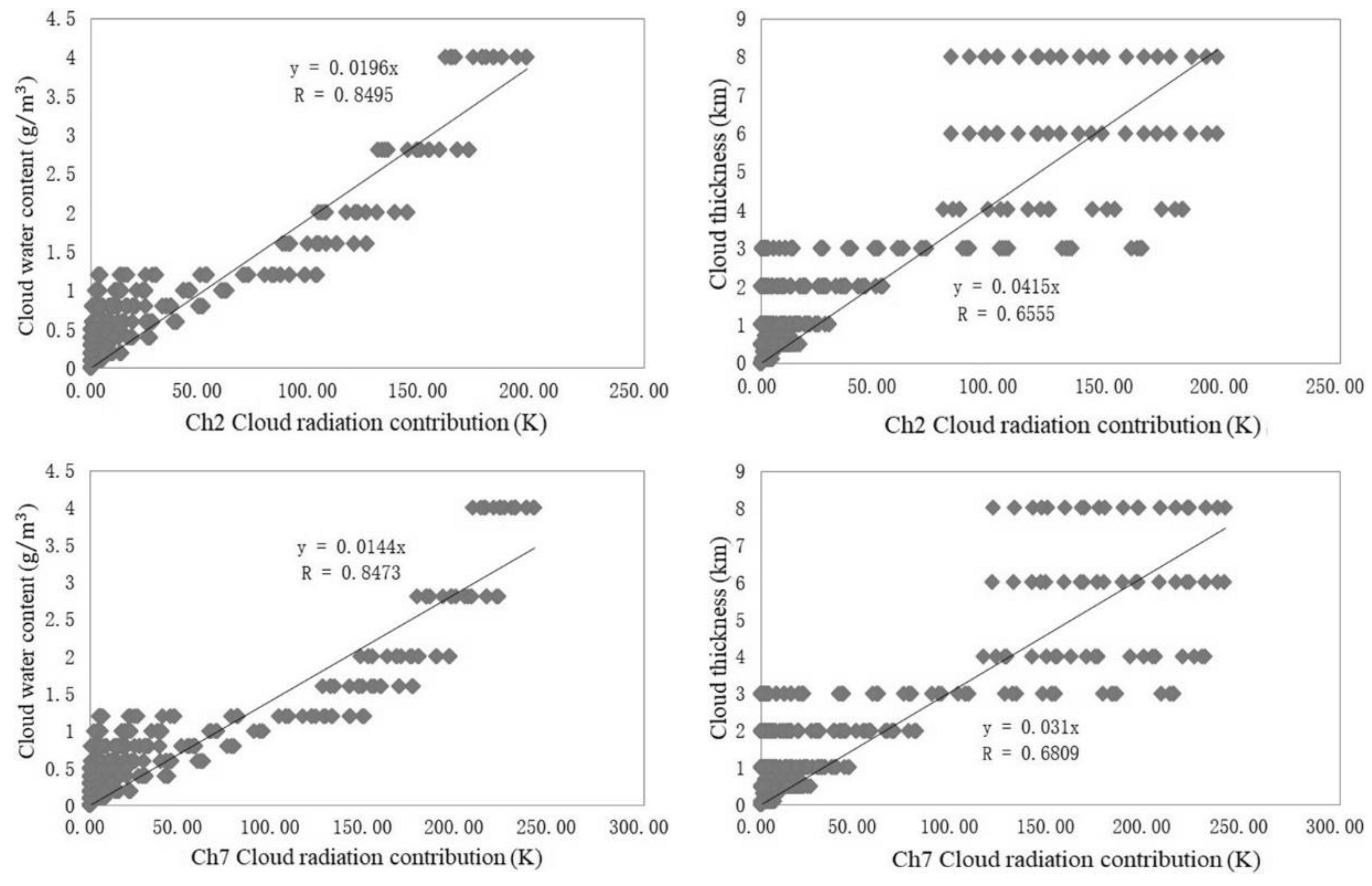
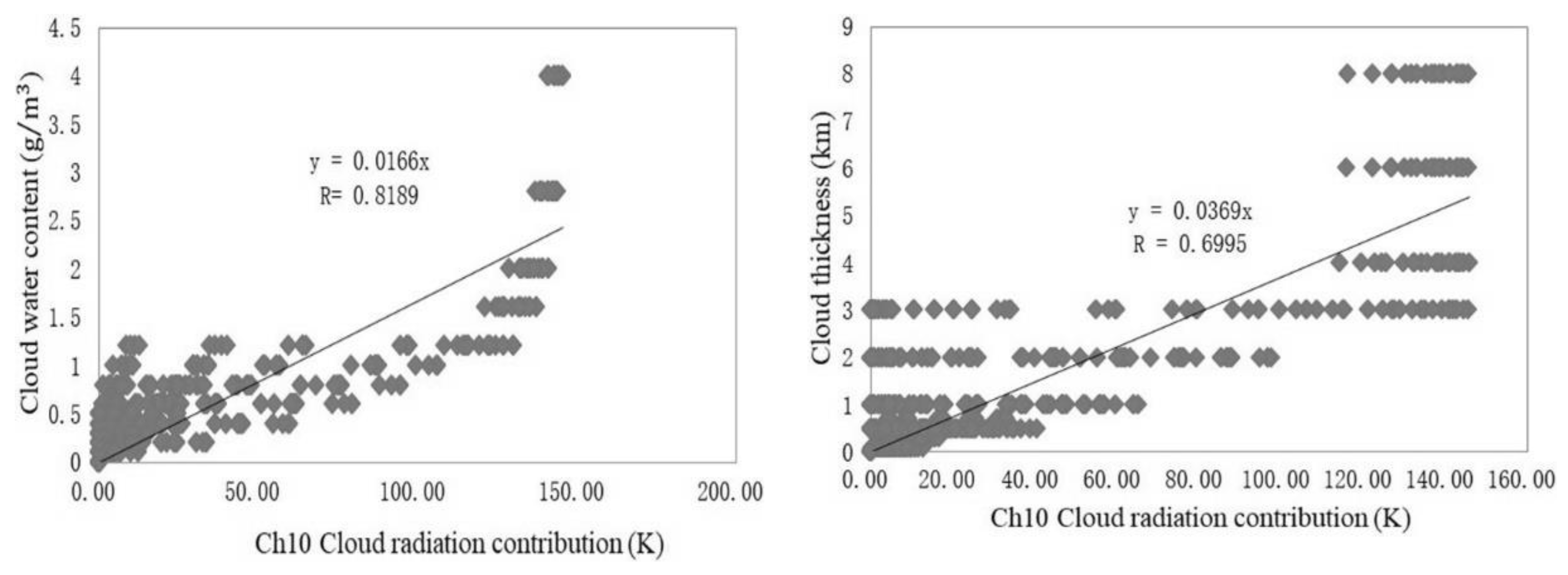
2.2. Method to Estimate Cloud Water Concentration and Cloud Thickness

Cloud water content can be obtained by microwave remote sensing [35] according to the transmission characteristics of microwaves in cloud [34,36,37]. Therefore, the study tries to obtain cloud water concentration and cloud thickness by using the few channels of the 22 in K and V bands. The method is as follows:

(1) Drawing on relevant cloud physics literature [38,39], we construct a parameter space comprising 800 possible cloud parameter combinations. As given in

Table 1. The 800 possible combinations of cloud parameter values based on the literature.

Cloud Types	Cloud Base Height ${\mathit{z}}_{\mathit{b}}\left(\mathbf{m}\right)$	Cloud Thickness $\Delta \mathit{H}\left(\mathbf{m}\right)$	Cloud Water Concentration $\mathit{M}$$(\mathit{g}/{\mathit{m}}^3)$	Total Number of Combinations	Cloud Impact Index (min, max)
Cumulus	500, 1000, 1500, 2000	100, 500, 1000, 2000	0.4, 0.6, 0.8, 1.0, 1.2	80	0.0200, 4.8
Cumulonimbus	500, 1000, 1500, 2000	3000, 4000, 6000, 8000	1.2, 1.6, 2.0, 2.8, 4.0	80	1.8000, 64
Stratocumulus	500, 1000, 2000, 2500	100, 500, 1000, 2000	0.2, 0.4, 0.6, 0.8, 1.0	80	0.0080, 4
Stratus	50, 200, 400, 800	100, 300, 500, 700	0.1, 0.2, 0.4, 0.6, 0.8	80	0.0125, 11.2
Nimbostratus	500, 1000, 1500, 2000	500, 1000, 2000, 3000	0.2, 0.4, 0.6, 0.8, 1.0	80	0.0500, 6
Altostratus	2000, 3000, 4000, 6000	100, 500, 1000, 2000	0.1, 0.2, 0.4, 0.6, 0.8	80	0.0017, 0.8
Altocumulus	2000, 3000, 4000, 6000	100, 500, 1000, 2000	0.1, 0.2, 0.4, 0.6, 0.8	80	0.0017, 0.8
Cirrus	4500, 6000, 8000, 10,000	500, 1000, 2000, 3000	0.1, 0.2, 0.3, 0.4, 0.5	80	0.0050, 0.3
Cirrostratus	4500, 6000, 8000, 9000	500, 1000, 2000, 3000	0.1, 0.2, 0.3, 0.4, 0.5	80	0.0056, 0.3
Cirrocumulus	4500, 6000, 7000, 8000	500, 1000, 2000, 3000	0.1, 0.2, 0.3, 0.4, 0.5	80	0.0063, 0.3

, ten types of clouds in meteorology are considered, with each cloud type having four possible cloud base heights, four thicknesses, and five possible cloud water concentrations.

(2) Based on the 1976 US standard atmosphere, a relative humidity of 95% is set at each height in the cloud to form a cloudy temperature and moisture layer. The forward calculation model represented by Equation (1) is used to obtain the calculated brightness temperature $T_{BC}$ and the calculated “presumed clear-sky” brightness temperature $T_{BCclear}$ (by setting $M=0$ and $\Delta H=0$). Then, according to Equation (4), the brightness temperature contribution of the cloud is:

$$\Delta T_B=T_{BC}-T_{BCclear}$$

(10)

(3) Analyze the sensitivity of the brightness temperature contribution of the cloud in each channel to cloud water concentration $M$ and cloud thickness $\Delta H$ in order to select the optimal channels. Scatter plots in Figure 1 show the sensitivity of $\Delta T_B$ to $M$ and $\Delta H$ for channels 2, 7 and 10, along with the associated correlation. Some of the points look fixed along the x-axis because they correspond to the dispersed values of cloud thickness and water content as shown by the third and fourth columns in Table 1, together with the cloud base height, as shown by the second column in Table 1, rather than only the 10 cloud types, as shown by the first column in Table 1. Among the 22 channels listed in

Table 2. Radiometer channel frequencies used for atmospheric temperature and humidity remote sensing.

Channel Index	Frequency (GHz)	Channel Index	Frequency (GHz)
1	22.23	2	22.50
3	23.03	4	23.83
5	25.00	6	26.23
7	28.00	8	30.00
9	51.20	10	51.76
11	52.28	12	52.80
13	53.34	14	53.85
15	54.40	16	54.94
17	55.50	18	56.02
19	56.66	20	57.29
21	57.96	22	58.80

, the cloud brightness temperature contribution in the band for channels 5–8 is physically the most suitable for cloud detection because the band is an atmospheric window, and followed by the band for channels 1–4 and the band for channels 9–15. The correlation is almost negligible at the channels of strong oxygen absorption. Taking into account the data independence of the atmospheric temperature and humidity inversion, the middle channel of each of these three bands (namely channels 2, 7 and 10) is selected to obtain cloud water concentration and cloud thickness. Until this point, a three-variable linear regression by foreseeing estimating coefficients collectively to provide minimum variance estimators is good enough to retrieve cloud water concentration and cloud thickness. However, one can see that the regression coefficients from the multiple linear regressions show a lack of stability since the channels are highly correlated with each other and are low correlated with the cloud parameters because of the nonlinearity shown by Equation (9a). To overcome this difficult situation, “the weighted average” is preferred, as detailed in the following steps.

(4) Cloud parameter inversion of a single channel. The theoretical relationship for the inversion is nonlinear, as shown by Equation (9a), and the scatterplots from the simulation to show the dependencies of cloud radiation contribution on cloud water content and cloud thickness are in Figure 1. Though a quadratic or cubic function would be better to obtain the best fitting according to the scatterplots of Figure 1, a linear function for simplicity has been used to obtain the regression model for inversing cloud water concentration and cloud thickness (denoted as $M_{1-3}$ and $\Delta H_{1-3}$) from $\Delta T_B$ of channel 2, 7 and 10:

$$M_i=a_i\Delta T_{B,j}+a{0}_i$$

(11a)

$$\Delta H_i=b_i\Delta T_{B,j}+b{0}_i$$

(11b)

where $a$, $a0$, $b$ and $b0$ are regression coefficients, and subscript $i$ = 1, 2, and 3 corresponds to channel $j$ = 2, 7 and 10, respectively.

(5) Establish a cloud parameter estimation model with a three-channel combined weighted average. To improve the reliability of the estimated cloud parameters for the brightness temperature correction calculation, the single-channel inversion results $M_{1-3}$ and $\Delta H_{1-3}$ obtained in the previous step are combined to obtain weighted averages:

$$M=\frac{M_1\frac{1}{W_{1,1}}+M_2\frac{1}{W_{1,2}}+M_3\frac{1}{W_{1,3}}}{\frac{1}{W_{1,1}}+\frac{1}{W_{1,2}}+\frac{1}{W_{1,3}}}$$

(12a)

$$\Delta H=\frac{\Delta H_1\frac{1}{W_{2,1}}+\Delta H_2\frac{1}{W_{2,2}}+\Delta H_3\frac{1}{W_{2,3}}}{\frac{1}{W_{2,1}}+\frac{1}{W_{2,2}}+\frac{1}{W_{2,3}}}$$

(12b)

where $W_{1,1-3}$ and $W_{2,1-3}$ are the standard deviation of residuals from the regression analysis to obtain Equation (11) for the individual channel. See the left side of Figure 2a.

It must be pointed that the cloud parameters obtained by the procedure above are only used as parameters required for the brightness temperature correction in the inversion calculation for cloudy atmospheric profiles. If one wants to apply them for other purposes, a proper validation may be needed though the model (Equation (12)) is based on 800 possible cloud parameter combinations (shown in Table 1).

(6) Calculate the value of the Cloud Impact index. In this study, we define:

$$CI=\left(M\ast \Delta H\right)/\left(z_b+1\right)$$

(13)

as the Cloud Impact index. The digit “1” in the denominator is for the situation that $z_b$ from TIR equals to zero for very low cloud. The value ranges of the CI shown by the last column of Table 1 indicate that the value of CI defined by Equation (13) may be as large as 64 for cumulonimbus, though it is close to 0 in most cases. The higher values correspond to the lower, thicker and denser clouds, which block the down-ward radiance in a more efficient manner. The larger the value of CI, the more necessary we make cloud correction though the more difficulty we have. Obviously, CI is equal or close to zero in the case when cloud impact can be neglected and TB correction for the cloud is not necessary.

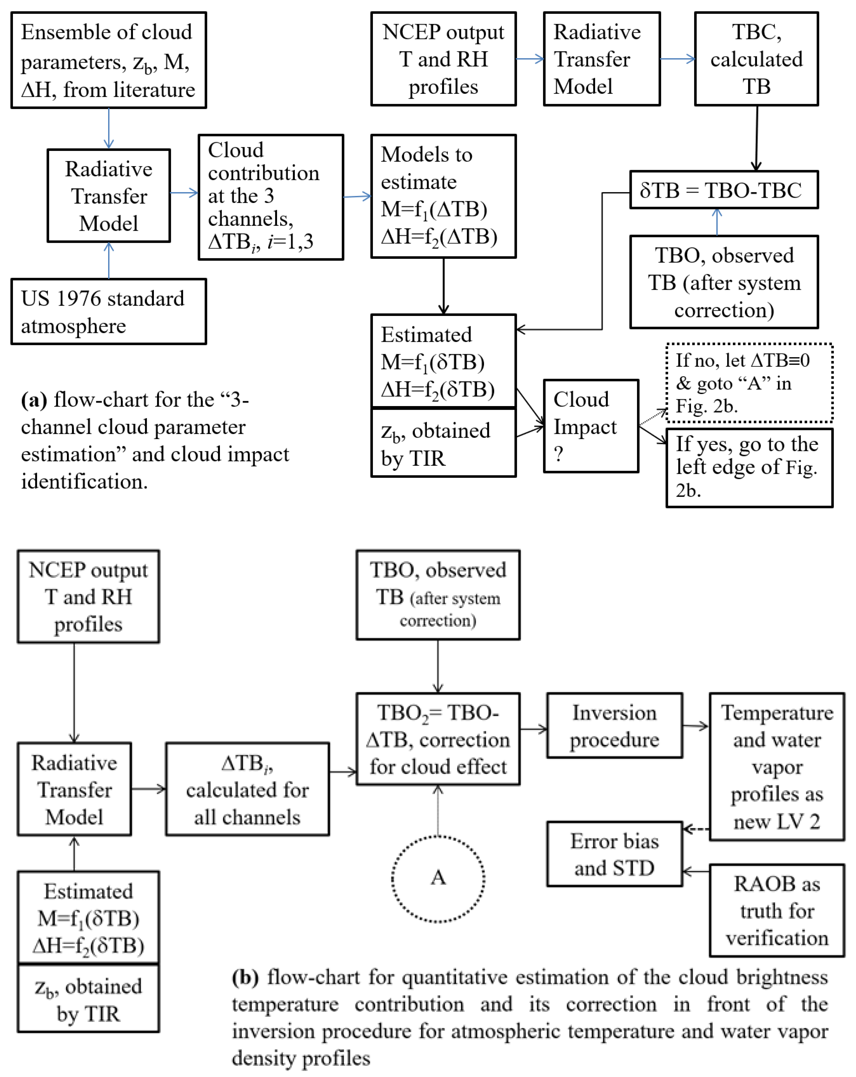
2.3. Algorithm for Atmospheric Temperature and Humidity Profile Inversion in Cloudy Conditions

In this work, the influence of cloud on brightness temperatures is corrected before the procedure of the inversion for atmospheric temperature and humidity profiles. The specific algorithm steps are as follows:

(1) The atmospheric vertical profile in NCEP-fnl (the final analysis data provided by the National Centers for Environmental Prediction and the National Centre for Atmospheric Research of United States) is substituted into the radiation transfer model (Equation (1)) to estimate the “presumed clear-sky” atmospheric contribution $T_{BCclear}$ for channels 2, 7 and 10. See the upper-right part of Figure 2a.

(2) Calculate the cloud influence on brightness temperature in channels 2, 7 and 10. Based on Equation (4), this quantity is given by:

$$\mathsf{\delta }{T}_{Bj}=T_{BO,j}-T_{BCclear,j}$$

(14)

where $j$ = 2, 7, 10, and $T_{BO,j}$ is the observed brightness temperature in the respective channel. If there is a systematic deviation in the original LV1 data, $T_{BO}$ in Equation (13) is the brightness temperature after systematic correction. The same applies below.

(3) Calculate the cloud parameters M and ∆H. Substituting $\mathsf{\delta }{T}_B$ obtained in the previous step into Equations (11) and (12) gives the inversion values of cloud water concentration and cloud thickness, as shown by the lower-right part of Figure 2a.

(4) Separate clear-sky and cloudy-sky cases in the observed data. Cloudy-sky cases are defined as when infrared temperature from TIR is >250 K, and the cloud parameters inversed from Equation (12) are greater than 0. The following steps are only applied to cloudy samples.

(5) Calculate the value of the Cloud Impact index with the estimated cloud water concentration and cloud thickness, together with the cloud base height from TIR. As shown above, CI is equal or close to zero in the case when cloud impact can be neglected and TB correction for cloud is not necessary, as shown by the dotted box in Figure 2a, which leads to a “goto” circled A shown in Figure 2b.

(6) Simulate the observed cloud-sky brightness temperature $T_{BC}$ of each channel. The cloud water concentration $M$, the cloud thickness $\Delta H$, and the cloud base height $z_b$ obtained by the infrared sensor inversion, along with the atmospheric temperature and humidity vertical profiles from NCEP are all substituted into the radiation transfer model (Equation (1), and the simulated brightness temperature $T_{BC}$ of each channel is obtained.

(7) Calculate the cloud influence on brightness temperature in all channels. Based on Equation (10), this quantity is:

$$\Delta T_B=T_{BC}-T_{BCclear}$$

(15)

(8) The “clear-sky atmospheric contribution” in the bright temperature of all channels can be obtained. Based on Equation (4), the clear-sky contribution is:

$$T_{BO2}=T_{BO}-\Delta T_B$$

(16)

where $T_{BO2}$ represents the LV1 brightness temperature data after correcting for the cloud influence. See the left side of Figure 2b for the last three steps above.

(9) $T_{BO2}$ from the 19 channels is used in the inversion of temperature and humidity profiles. The inversion method used in this study is the traditional, multiple regression method [21,40,41], and the regression coefficients are calculated from clear-sky observations.

One can see that the NCEP atmospheric vertical profiles have been used in the above process, and acts as “the initial atmospheric state”. The estimated cloud parameters are obtained using $T_{BO}$ from the three channels (channels 2, 7 and 10), and $T_{BO2}$ values from the remaining 19 channels are used to obtain cloud-corrected temperature and humidity profiles. Thereby, the atmospheric temperature and humidity states are more representative of their observational counterparts.

2.4. Verification of the Cloud Correction

Using radiosonde observations (RAOB) as “ground truth” values, the correlation coefficient, bias, and root-mean-square error at each height can be calculated to evaluate improvement in the inversion results due to the method presented by this study, as shown by the right side of Figure 2b. The RAOB temperature or water vapor density profile (at a total of L = 58 height layers) is denoted by the vector $\stackrel{\rightharpoonup }{f}$,

$$\stackrel{\rightharpoonup }{f}={\left[T_1,T_2,\cdots T_L\right]}^T$$

(17)

Additionally, the vector

$$\stackrel{\rightharpoonup }{\widehat{f}}={\left[{\widehat{T}}_1,{\widehat{T}}_2,\cdots {\widehat{T}}_L\right]}^T$$

(18)

denotes either the corresponding LV2 data product provided by the render (${\stackrel{\rightharpoonup }{\widehat{f}}}_{-}\mathrm{LV}2$) or the inversion results from this study (${\stackrel{\rightharpoonup }{\widehat{f}}}_{-}{T}_{BO2}$). The $\stackrel{\rightharpoonup }{f}$ and $\stackrel{\rightharpoonup }{\widehat{f}}$ for the whole sample are expressed as matrices:

$$F={\left[T_{ln}\right]}_{L\times N}$$

(19)

$$\widehat{F}={\left[{\widehat{T}}_{ln}\right]}_{L\times N}$$

(20)

where N is the sample size. The error in the nth estimated profile at the lth height layer is given by:

$$e_{ln}={\widehat{T}}_{ln}-T_{ln}$$

(21)

The correlation coefficient, bias, and root-mean-square error at the lth height layer are, respectively,

$$R_l=\frac{{\displaystyle \sum _{n=1}^N\left(T_{ln}-{\overline{T}}_l\right)\left({\widehat{T}}_{ln}-{\overline{\widehat{T}}}_l\right)}}{\sqrt{{\displaystyle \sum _{n=1}^N{\left(T_{ln}-{\overline{T}}_l\right)}^2}}\sqrt{{\displaystyle \sum _{n=1}^N{\left({\widehat{T}}_{ln}-{\overline{\widehat{T}}}_l\right)}^2}}}$$

(22)

$$BIA{S}_l=\frac{1}{N}{\displaystyle \sum _{n=1}^N{e}_{ln}}$$

(23)

$$RMS{E}_l=\sqrt{\frac{1}{N}{\displaystyle \sum _{n=1}^N{\left(e_{ln}-BIA{S}_l\right)}^2}}$$

(24)

where ${\overline{\widehat{T}}}_l=\frac{1}{N}{\displaystyle \sum _{n=1}^N{\widehat{T}}_{ln}}$ and ${\overline{T}}_l=\frac{1}{N}{\displaystyle \sum _{n=1}^N{T}_{ln}}$. The larger the correlation coefficient, the better the consistency in the time variation between $\stackrel{\rightharpoonup }{\widehat{f}}$ and $\stackrel{\rightharpoonup }{f}$. The closer the bias and root mean square are to zero, the smaller the error in $\stackrel{\rightharpoonup }{\widehat{f}}$ relative to $\stackrel{\rightharpoonup }{f}$. That is, the larger the correlation coefficient, and the closer the error deviation and the root mean square are to zero, the better the consistency between the radiosonde observations and the inversion results of the LV2 data or $T_{BO2}$.

3. Data

The LV1 data together with the corresponding LV2 products from a radiometer in Beijing are collected twice a day at 00:00 and 12:00 UTC between January 2010 and December 2011. The NCEP-fnl data for time matching with the radiometer twice a day at 00:00 and 12:00 UTC, have a spatial resolution of 1° × 1°, and the grid point used in the calculation is at (40° N, 116° E) which is the closest to the position of the radiometer (40°07′ N, 116°36′ E). And the RAOB station (39°55′ N, 116°16′ E) to provide the “truth” for verification in this study is about 36 km away from the radiometer.

According to the method given by the fourth step in Section 2.3, the final sample size of “cloudy-sky” in Beijing’s two-years data is 109, considering that the radio sounding is performed twice a day. The observed brightness temperature data of the 22 channels are noted as $T_{BO}$ after systematic deviation correction [21]. The brightness temperatures $T_{BO2}$ of the 109 cloudy-sky cases that passed both the system deviation correction and the cloud effect correction were then applied to reverse the temperature and water vapor density of the cloudy sky, as described by the ninth step in Section 2.3.

4. Results

The temperature and water vapor density profiles retrieved from $T_{BO2}$ for the 109 cloudy sky cases are compared to the RAOB to calculate the errors, error statistics, and correlation coefficient at each height according to the method described in Section 2.4. This section gives the results from the statistical analysis of the errors, the cases analysis, and the performance analysis of the method under different cloud types.

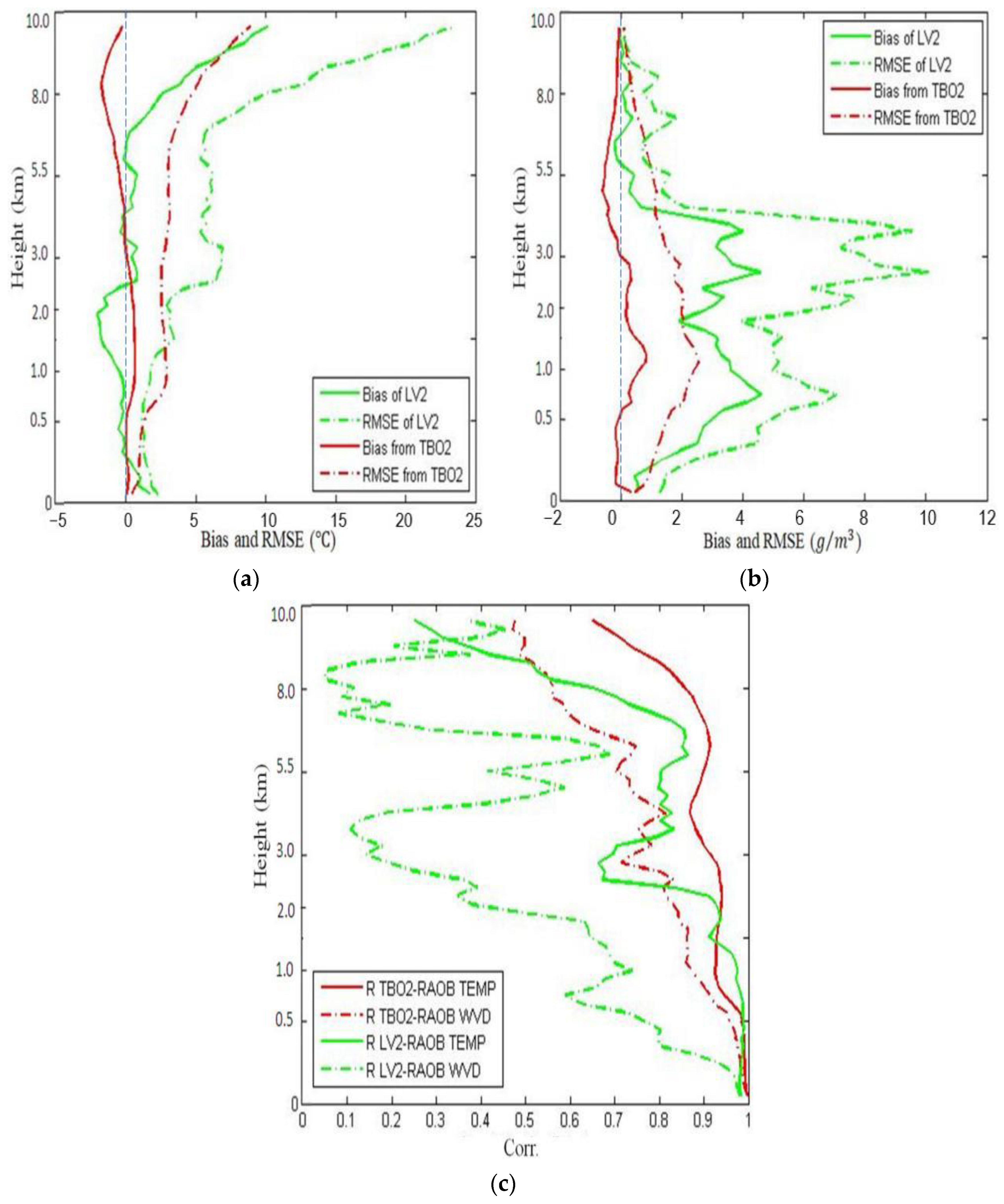
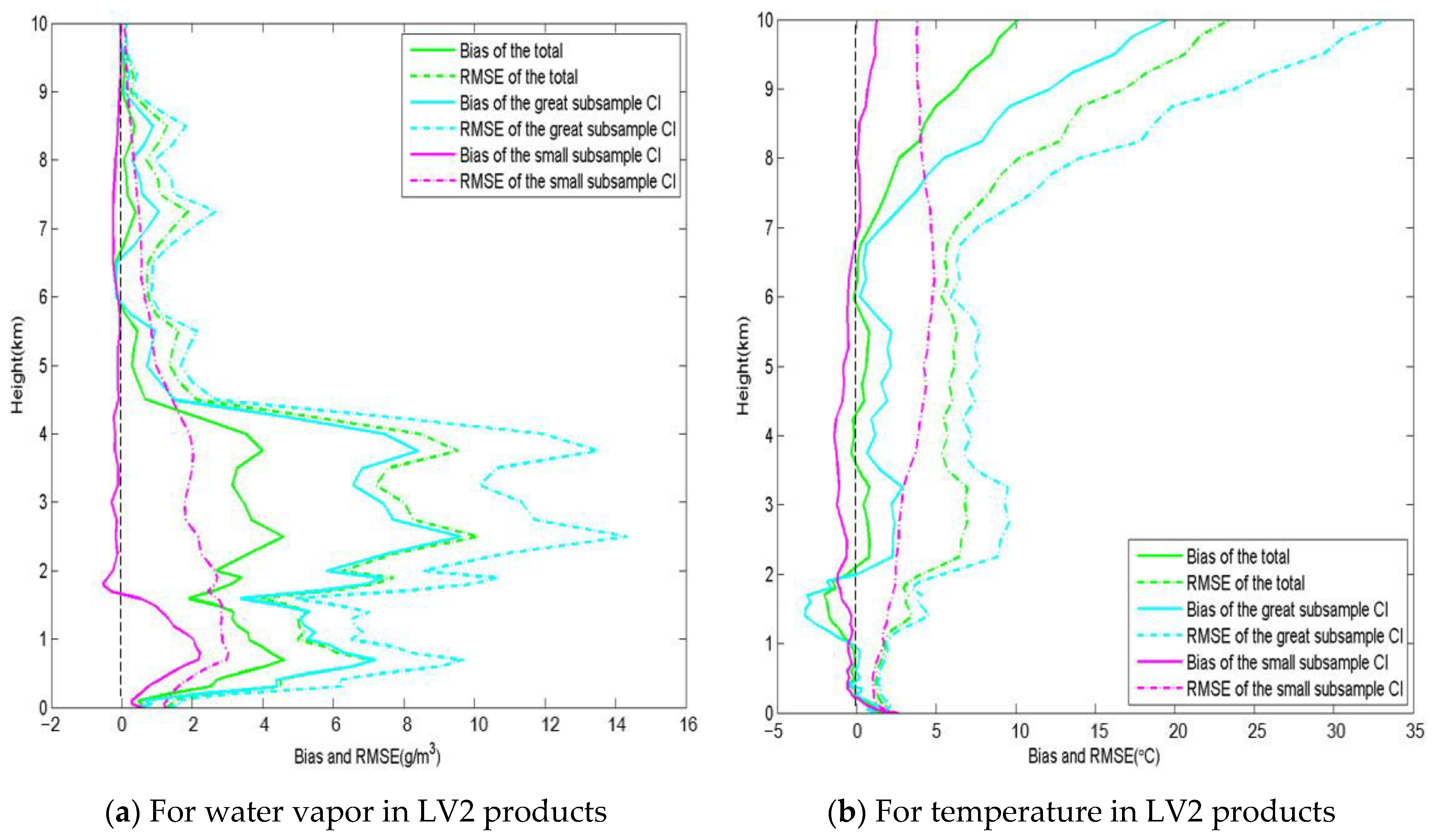
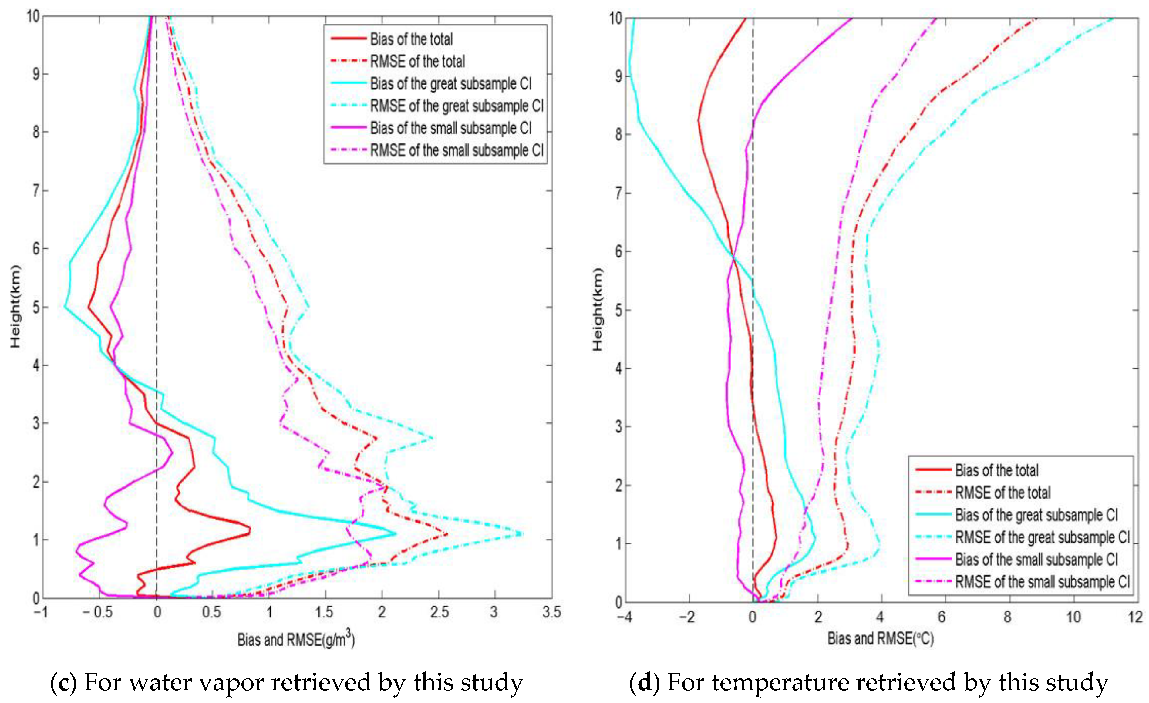
4.1. Statistical Comparison of the Errors in the Retrieved Profiles

The bias and RMSE (root mean square error) of the temperature and water vapor density profiles from the cloudy-sky $T_{BO2}$ inversions (red lines) from this study for the 109 cloudy cases (Sample size = 109) are shown in Figure 3 as red lines, together with the corresponding errors in the original, vendor-provided LV2 data (green lines). The y-ordinate of Figure 3 uses piecewise linear regression to make it easier to see the vertical variation of the statistics in the middle and lower atmosphere.

One can see that the errors in the results from this study are notably smaller than in the vendor-provided LV2. The bias of the temperature profile (see the solid, red curve in Figure 3a) from this study is close to zero (see the black, dashed line as a reference line at zero) at all heights, and the RMSE is greatly reduced from >5 °C to <2 °C above 1.5 km. The bias of the water vapor density profile from this study (see the solid, red curve in Figure 3b) is near to 0 while the LV2 has a positive bias as large as 4 g/m³ (see the solid, green curve in Figure 3b). The RMSE of the water vapor density profile from this study (see the dashed, red curve in Figure 3b) is <2 g/m³ while the RMSE for LV2 is as large as 10 g/m³ (see the dashed, green curve in Figure 3b). That is, both the bias and RMSE from this study are evidently less than the LV2, with greater improvement in the lower troposphere below 5 km. The temperature retrievals from this study have a higher correlation with the RAOB data compared to the vendor-provided LV2 (Figure 3c), especially at and above a 2 km height. Correlation with RAOB is improved even more for the water vapor density. The correlation of LV2 with RAOB is only 0.8 at 0.5 km height, 0.7 at 1 km, and even less than 0.5 at 2 km, but the correlation of the retrievals from this study increases to 1 within the boundary layer. These results indicate that the method presented by this study can effectively improve the consistency between the inversion results and radiosonde measurements.

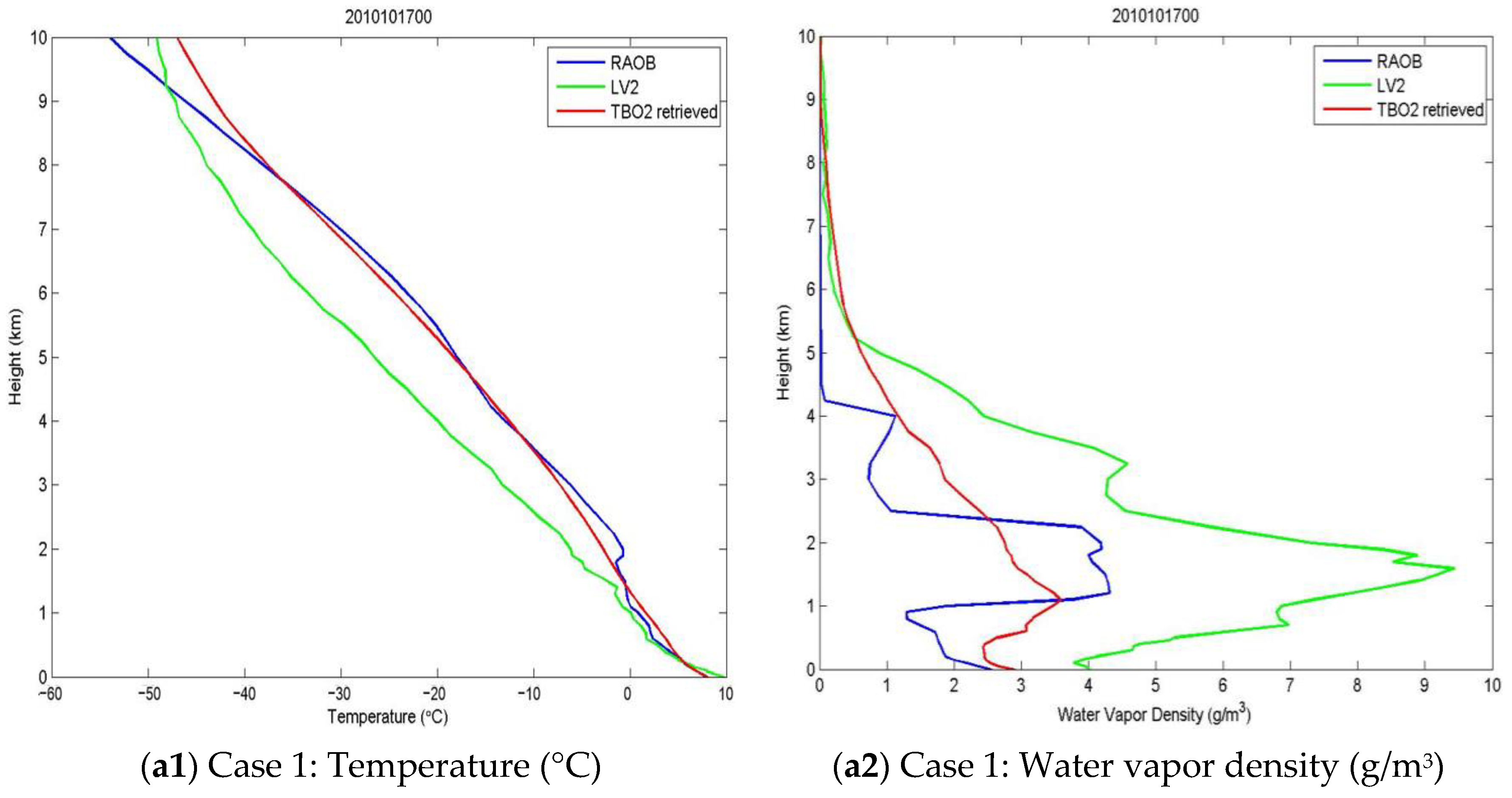
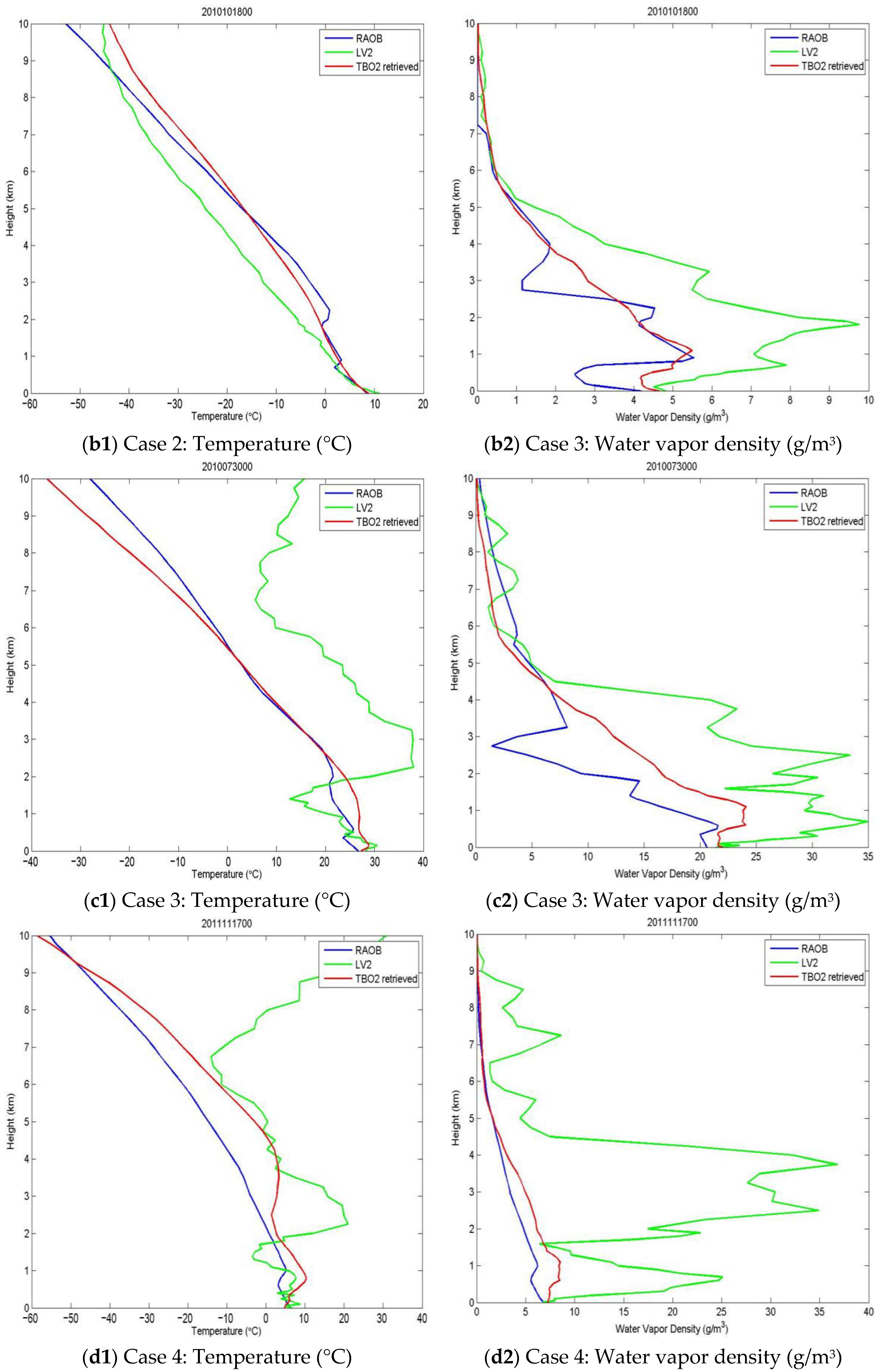
4.2. Cases Comparison of the Retrieved Profiles with the RAOB

Four typical cases are given in Figure 4 to make a comparison among the atmospheric profiles retrieved from this study (i.e., ${\stackrel{\rightharpoonup }{\widehat{f}}}_{-}{T}_{BO2}$), the vendor-provided LV2, and RAOB.

The first two cases are typical for early winter in Beijing, where the surface air temperature is about 10 °C and the humidity is around 5 g/m³. There exists a layer of stratus or stratocumulus at the level of 2–3 km. The cloud layer may be revealed by RAOB because the humidity inside the cloud is larger than the outside but the temperature decreases smoothly as height increases in the troposphere. The features above are shown well by the blue lines for RAOB in Figure 4a,b. The two cases differ in time by 24 h, but look similar, implying that the information from RAOB is reliable. The ${\stackrel{\rightharpoonup }{\widehat{f}}}_{-}{T}_{BO2}$ temperature profiles (red line in Figure 4(a1,b1)) are obviously closer to the RAOB than the LV2, especially above 2 km where agreement is particularly strong. The water vapor density profiles ${\stackrel{\rightharpoonup }{\widehat{f}}}_{-}{T}_{BO2}$ (red line in Figure 4(a2,b2)), although different from the RAOB, is in better agreement with the RAOB than the LV2, which led the water vapor density overestimated up to 10 g/m³, as compared to the truth of 4–5 g/m³.

Case 3 at 00:00 UTC on 30 July 2010 is typical for summer in Beijing, where the surface air is around 30 °C and the humidity may reach as high as 20–25 g/m³. Low and thick clouds such as cumulus and cumulonimbus may exist. In this situation, LV2 would give an even more humid (water vapor density close to 35 g/m³) and warmer air (temperature as high as 40 °C at some levels). The information from LV2 is obviously unrealistic and must be wrong.

Case 4, as shown in Figure 4d, is for winter in late 2011, but the LV2 appears similar to that in Case 3 for summer. The optically thick clouds associated with trough and cyclone systems may happen in winter as well as in summer. Obviously the LV2 profiles in this situation would be repeatedly unrealistic and must be wrong.

All the retrievals for the 109 cloud cases have been checked out and many cases like Cases 3 and 4 have been found, i.e., the error in LV2 is too large, which has just been reflected by the statistics of errors given in Figure 3. Generally speaking, (1) Thick dense clouds influence the retrievals more than the thin clouds because of considerable attenuation, and (2) for a given cloud thickness, lower clouds influence more than high clouds because of the weighting function, which always decreases as the height increases for ground-based remote sensing. The method presented by this paper for cloud correction would improve the retrievals for low, thick and dense clouds by a large amount even though the resident error is still large, as compared to that for high and thin clouds.

4.3. Performance under the Different Cloud Types

As defined and described in Section IIB, the value of CI, the cloud impact index, which depends on the three-channel estimated cloud water concentration, cloud geometric thickness and the cloud-base height from TIR, has been computed for all the 109 cloudy cases. High CI means that the case is a high impact cloud case, cloud effect is large, and the difficulty to make correction would be increased. Low CI means that the case is a low impact cloud case, and it might be easier to make a satisfying correction. The whole sample with 109 cloudy cases is sliced into two sub-samples according to CI values in order to see the performance of the method presented by this study under the different cloud situations by looking at the sub-sample difference in error statistics, as given in Figure 5.

The upper two sub-panels in Figure 5 are for the accuracy of water vapor density (Figure 5a) and temperature (Figure 5b) in the vendor- provided LV2 products. Green lines, as shown before in Figure 3, represent the LV2 ensemble accuracy of the total 109 cloudy cases. However, the cyan lines represent the subsample accuracy for high-CI cases, while the magenta lines represent the subsample accuracy for low-CI cases. One can see that both BIAS and RMSE of “high-CI subsample” are larger than those of “low-CI subsample”, indicating that high-CI cloud has a higher impact on the retrieved results and cloud correction is more necessary.

The lower two sub-panels (Figure 5c,d) are for the accuracy of water vapor density and temperature retrieved by this study. Red lines, as shown above in Figure 3, represent the accuracy of the retrievals from this study for all the 109 cloud cases. The cyan lines and the magenta lines are for high-CI and low-CI subsamples, respectively. One can see that both BIAS and RMSE of “high-CI subsample” are again larger than those of “low-CI subsample”, indicating that high-CI cloud correction is more difficult. Comparison of Figure 5c,d with Figure 5a,b shows that the BIAS and RMSE in the lower two sub-panels are much less than those in the upper two sub-panels. In the water vapor density figures, the BIAS was reduced from 9.6 to 0.5 around the height of 2.5 km, and the RMSE was reduced from 14.3 to 3.3. The accuracy of retrieved temperature is also evidently improved by this study, especially at the height above 2 km.

5. Conclusions and Suggestions

This paper presented an approach to improve the retrievals of cloudy atmospheric profiles from ground-based microwave radiometer observations. In terms of both radiative transfer and statistic features of clouds, a “three-channel method” has been suggested to use the three cloud-sensitive channels of the radiometer itself to quantitatively make cloud parameter estimation and apply it to microwave brightness temperature inversion to obtain a new retrieval of atmospheric profiles so that the new retrievals would be closer to the radiosonde and evidently better than the LV2 provided by the vendor. The results from this study on the two years data obtained in Beijing demonstrate that the method works well in cloudy cases for improving temperature and humidity retrievals according the verification with RAOB, as compared to the vendor-provided LV2 products.

(1) The temperature retrievals from this study have higher correlation with RAOB and are notably better than in the vendor-provided LV2. The bias of the temperature retrievals from this study is close to zero at all heights, and the RMSE is greatly reduced from >5 °C to <2 °C in the layer from about 1.5 km up to 5 km. The temperature retrievals from this study have a higher correlation with RAOB data compared to the vendor-provided LV2 (Figure 3c), especially at and above 2 km height.

(2) The bias of the water vapor density profile from this study is near to 0, while the LV2 has a positive bias as large as 4 g/m³. The RMSE of the water vapor density profile from this study is <2 g/m³ while the RMSE for LV2 is as large as 10 g/m³. That is, both the bias and RMSE from this study are evidently less than the LV2, with greater improvement in the lower troposphere below 5 km. Correlation with RAOB is improved even more for the water vapor density. The correlation of LV2 with RAOB is only 0.8 at 0.5 km height, 0.7 at 1 km, and even less than 0.5 at 2 km, but the correlation of the retrievals from this study increases to 1 within the boundary layer.

(3) A parameter named as Cloud Impact index, determined by cloud water concentration and cloud thickness together with the cloud base height, has been defined to indicate the fact that the larger the CI, the more necessary to make cloud correction though the more difficulty one has. The whole sample with 109 cloudy cases was sliced into two sub-samples according to CI values in order see the sub-sample difference in error statistics and the results show that both BIAS and RMSE of “high-CI subsample” are larger than those of “low-CI subsample”, indicating that high-CI cloud has a higher impact on the retrievals and the correction for cloud influence is more necessary.

The large error in the original LV2 may be caused by the different a priori dataset for training. It is hoped that the LV2 can be improved by expanding the training dataset, e.g., to include more cases of thick cloud. However, it is also hoped that the idea in this study can be taken as a reference for those who need to solve the cloud problem, though some approximations and simplifications in the study and the geo-position difference of the datasets for comparison may cause additional errors.

Of cause the method presented by this paper for cloud correction has limitations such as the following.

(1) The method requires that the number of channels of the radiometer must be great enough. Otherwise, the number of channels for temperature and humidity profile retrievals would not be enough because three channels has been used for cloud correction in advance.

(2) The method still depends on the thermal infrared sensor on board the microwave radiometer to provide cloud base height. The uncertainty in thermal infrared sensor would influence the results from this method.

References

1. Liang, L.; Li, X.; Zheng, F. Spatio-Temporal Analysis of Ice Sheet Snowmelt in Antarctica and Greenland Using Micro-wave Radiometer Data. Remote Sens. 2019, 11, 1838. [Google Scholar] [CrossRef] [Green Version]
2. Gonzalez, S.; Bech, J.; Udina, M.; Codina, B.; Paci, A.; Trapero, L. Decoupling between Precipitation Processes and Mountain Wave Induced Circulations Observed with a Vertically Pointing K-Band Doppler Radar. Remote Sens. 2019, 11, 1034. [Google Scholar] [CrossRef] [Green Version]
3. Liu, L.; Ruan, Z.; Zheng, J.; Gao, W. Comparing and Merging Observation Data from Ka-Band Cloud Radar, C-Band Frequency-Modulated Continuous Wave Radar and Ceilometer Systems. Remote Sens. 2017, 9, 1282. [Google Scholar] [CrossRef] [Green Version]
4. Ware, R.; Carpenter, R.; Güldner, J.; Liljegren, J.; Nehrkorn, T.; Solheim, F.; Vandenberghe, F. A multichannel radiometric profiler of temperature, humidity, and cloud liquid. Radio Sci. 2003, 38, 8079. [Google Scholar] [CrossRef] [Green Version]
5. Won, H.Y.; Kim, Y.H.; Lee, H.S. An application of brightness temperature received from a ground-based microwave radiometer to estimation of precipitation occurrences and rainfall intensity. Asia-Pac. J. Atmos. Sci. 2009, 45, 55–69. [Google Scholar]
6. Barrere, C.A.; Eilts, M.; Johnson, J.; Fritchie, R.; Spencer, P.; Shaw, B.; Li, Y.; Ladwig, W.; Schudalla, R.; Mitchell, D. An Aviation Weather Decision Support System (AWDSS) for the Dubai International Airport. In Proceedings of the 13th Conference on Aviation, Range, and Aer-ospace Meteorology, New Oeleans, LA, USA, 20–24 January 2008; pp. 20–24. Available online: https://www.researchgate.net/publication/228958651_An_Aviation_Weather_Decision_Support_System_AWDSS_for_the_Dubai_International_Airport (accessed on 24 January 2019).
7. Raju, C.S.; Renju, R.; Antony, T.; Mathew, N.; Moorthy, K.K. Microwave Radiometric Observation of a Waterspout Over Coastal Arabian Sea. IEEE Geosci. Remote Sens. Lett. 2013, 10, 1075–1079. [Google Scholar] [CrossRef]
8. Gültepe, I.; Kuhn, T.; Pavolonis, M.; Calvert, C.; Gurka, J.; Heymsfield, A.J.; Liu, P.S.K.; Zhou, B.; Ware, R.; Ferrier, B.; et al. Ice Fog in Arctic During FRAM–Ice Fog Project: Aviation and Nowcasting Applications. Bull. Am. Meteorol. Soc. 2014, 95, 211–226. [Google Scholar] [CrossRef] [Green Version]
9. Pan, Y.; Zhang, S.; Li, Q.; Ma, L.; Jiang, S.; Lei, L.; Lyu, W.; Wang, Z. Analysis of convective instability data derived from a ground-based microwave radiometer before triggering operations for artificial lightning. Atmos. Res. 2020, 243, 105005. [Google Scholar] [CrossRef]
10. Li, J.; Guo, L.X.; Lin, L.K.; Zhao, Y.; Zhao, Z.; Shu, T.; Han, H. A Dual-Frequency Method of Eliminating Liquid Water Ra-diation to Remotely Sense Cloudy Atmosphere by Ground-Based Microwave Radiometer. Prog. Electromagn. Res. 2013, 138, 629–645. [Google Scholar] [CrossRef] [Green Version]
11. d’Auria, G.; Marzano, F.S.; Pierdicca, N.; Nossai, R.P.; Basili, P.; Ciotti, P. Remotely sensing cloud properties from micro-wave radiometric observations by using a modeled cloud database. Radio Sci. 1998, 33, 369–392. [Google Scholar] [CrossRef]
12. Zhu, Y.J.; Hu, C.D.; Zhen, J.M.; Zhao, B.L. The Role of Microwave Radiometer in Weather Modification Research. Acta Sci. Nat. PKU 1994, 30, 597–606. [Google Scholar]
13. Guo, L.J.; Guo, X.L. Verification study of the atmospheric temperature and humidity profiles retrieved from the ground-based multi-channels microwave radiometer for persistent foggy weather events in northern China. Acta Meteorol. Sin. 2015, 73, 368–381. (In Chinese) [Google Scholar]
14. Heggli, M.; Rauber, R.M.; Snider, J.B. Field Evaluation of a Dual-Channel Microwave Radiometer Designed for Measurements of Integrated Water Vapor and Cloud Liquid Water in the Atmosphere. J. Atmos. Ocean. Technol. 1987, 4, 204–213. [Google Scholar] [CrossRef] [Green Version]
15. Revercomb, H.E.; Turner, D.D.; Tobin, D.C.; Splitt, M.E. The Arm Program’s Water Vapor Intensive Observation Peri-ods. Bull. Am. Meteorol. Soc. 2003, 84, 217–236. [Google Scholar] [CrossRef]
16. Cadeddu, M.P.; Liljegren, J.C.; Turner, D.D. The Atmospheric Radiation Measurement (ARM) program network of mi-crowave radiometers: Instrumentation, data, and retrievals. J. Atmos. Ocean. Technol. 2013, 29, 1182–1201. [Google Scholar]
17. Cimini, D.; De Angelis, F.; Dupont, J.-C.; Pal, S.N.; Haeffelin, M. Mixing layer height retrievals by multichannel microwave radiometer observations. Atmos. Meas. Tech. 2013, 6, 2941–2951. [Google Scholar] [CrossRef] [Green Version]
18. Li, Q.; Hu, F.C.; Chu, Y.L.; Wang, Z.H.; Huang, J.S.; Wang, Y. A Consistency Analysis and Correction of the Brightness Temperature Data Observed with a Ground-based Microwave Radiometer in Beijing. Remote Sens. Technol. Appl. 2014, 29, 547–556. (In Chinese) [Google Scholar]
19. Wang, Z.H.; Li, Q.; Chu, Y.L.; Zhu, Y.Y. Environmental Thermal Radiation Interference on Atmospheric Brightness Temperature Measurement with Ground-based K-band Microwave Radiometer. J. Appl. Meter. Sci. 2014, 25, 711–721. (In Chinese) [Google Scholar]
20. Li, Q.; Wei, M.; Wang, Z.H.; Chu, Y.L.; Ma, L.N. Evaluation and Correction of Ground-Based Microwave Radiometer Ob-servations Based on NCEP-FNL Data. Atmos. Clim. Sci. 2019, 9, 229–242. [Google Scholar]
21. Li, Q.; Wei, M.; Wang, Z.; Chu, Y. Evaluation and Improvement of the Quality of Ground-Based Microwave Radiometer Clear-Sky Data. Atmosphere 2021, 12, 435. [Google Scholar] [CrossRef]
22. Hu, S.Z.; Ma, S.Q.; Ta, F.; Qin, Y.; Guo, W.; Wen, X.G. Ground based Dual band Cloud Observing System and Its Compar-ative Experiments. J. Appl. Meteorol. Sci. 2012, 23, 441–450. (In Chinese) [Google Scholar]
23. Hewison, T.J. 1D-VAR retrieval of temperature and humidity profiles from a ground-based microwave radiometer. IEEE Trans. Geosci. Remote 2007, 45, 2163–2168. [Google Scholar] [CrossRef]
24. Knupp, K.R.; Coleman, T.; Phillips, D. Ground-based passive microwave profiling during dynamic weather condi-tions. J. Atmos. Ocean. Technol. 2009, 26, 1057–1073. [Google Scholar] [CrossRef]
25. Che, Y.; Ma, S.; Xing, F.; Li, S.; Dai, Y. An improvement of the retrieval of temperature and relative humidity profiles from a combination of active and passive remote sensing. Meteorol. Atmos. Phys. 2019, 131, 681–695. [Google Scholar] [CrossRef]
26. Zhang, X.; Wang, Z.; Mao, J.; Wang, Z.; Zhang, G.; Tao, F. Experiments on improving temperature and humidity profile retrieval for ground-based microwave radiometer. J. Appl. Meteor. Sci. 2020, 31, 385–396. (In Chinese) [Google Scholar]
27. Jiang, J.H.; Yue, Q.; Su, H.; Kangaslahti, P.; Lebsock, M.; Reising, S.; Schoeberl, M.; Wu, L.; Herman, R.L. Simulation of Remote Sensing of Clouds and Humidity From Space Using a Combined Platform of Radar and Multifrequency Microwave Radiometers. Earth Space Sci. 2019, 6, 1234–1243. [Google Scholar] [CrossRef] [Green Version]
28. Stankov, B.B. Ground- and Space-Based Temperature and Humidity Retrievals: Statistical Evaluation. J. Appl. Meteorol. 1996, 35, 444–463. [Google Scholar] [CrossRef] [Green Version]
29. Bianco, L.; Cimini, D.; Marzano, F.S.; Ware, R. Combining Microwave Radiometer and Wind Profiler Radar Measurements for High-Resolution Atmospheric Humidity Profiling. J. Atmos. Ocean. Technol. 2005, 22, 949–965. [Google Scholar] [CrossRef] [Green Version]
30. Klaus, V.; Bianco, L.; Gaffard, C.; Matabuena, M.; Hewison, T. Combining UHF radar wind profiler and microwave radiometer for the estimation of atmospheric humidity profiles. Meteorol. Z. 2006, 15, 87–97. [Google Scholar] [CrossRef]
31. Barrera-Verdejo, M.; Crewell, S.; Löhnert, U.; Orlandi, E.; Di Girolamo, P. Ground-based lidar and microwave radiometry synergy for high vertical resolution absolute humidity profiling. Atmos. Meas. Tech. 2016, 9, 4013–4028. [Google Scholar] [CrossRef] [Green Version]
32. Han, Y.; Westwater, E.R. Remote Sensing of Tropospheric Water Vapor and Cloud Liquid Water by Integrated Ground-Based Sensors. J. Atmos. Ocean. Technol. 1995, 12, 1050–1059. [Google Scholar] [CrossRef] [Green Version]
33. Westwater, E.R.; Zhenhui, W.; Grody, N.C.; McMillin, L.M. Remote Sensing of Temperature Profiles from a Combination of Observations from the Satellite-Based Microwave Sounding Unit and the Ground-Based Profiler. J. Atmos. Ocean. Technol. 1985, 2, 97–109. [Google Scholar] [CrossRef] [Green Version]
34. Zhang, P.C.; Wang, Z.H. Fundamentals of Atmospheric Microwave Remote Sensing, 1st ed.; Meteorological Press: Beijing, China, 1995; pp. 306–307. (In Chinese) [Google Scholar]
35. Wei, C.; Lin, H.; Zou, S.X.; Xuan, Y.J. Microwave remote-sensing of atmospheric column water vapor and liquid water content of cloud over sea. J. Atmos. Sci. 1989, 13, 101–107. (In Chinese) [Google Scholar]
36. Resteghini, L.; Capsoni, C.; Luini, L.; Nebuloni, R. An Attempt to Classify the Types of Clouds by a Dual Frequency Mi-Crowave Radiometer. In Proceedings of the IEEE 13th Specialist Meeting on Microwave Radiometry and Remote Sensing of the Environment (MicroRad), Pasadena, CA, USA, 24–27 March 2014; pp. 90–93. Available online: https://ieeexplore_ieee.gg363.site/abstract/document/6878915 (accessed on 16 May 2021).
37. Erkelens, J.; Russchenberg, H.; Jongen, S.; Herben, M. Combining radar and microwave radiometer for cloud liquid water retrieval. In Proceedings of the IEEE 28th European Microwave Conference, Amsterdam, The Netherlands, 5–9 October 1998; pp. 67–72. [Google Scholar]
38. Karstens, U.; Simmer, C.; Ruprecht, E. Remote sensing of cloud liquid water. Theor. Appl. Clim. 1994, 54, 157–171. [Google Scholar] [CrossRef]
39. Hahn, J.; Warren, G.; London, J.; Chervin, M.; Jenne, R. Atlas of simultaneous occurrence of different cloud types over the ocean. Atmospheric Analysis and Prediction Division. Natl. Cent. Atmos. Res. 1982, 14–15. [Google Scholar] [CrossRef]
40. Karmakar, P.K.; Maiti, M.; Calheiros, A.J.P.; Angelis, C.F.; Machado, L.A.T.; Da Costa, S.S. Ground-based single-frequency microwave radiometric measurement of water vapour. Int. J. Remote Sens. 2011, 32, 8629–8639. [Google Scholar] [CrossRef] [Green Version]
41. Gentemann, C.L.; Meissner, T.; Wentz, F.J. Accuracy of Satellite Sea Surface Temperatures at 7 and 11 GHz. IEEE Trans. Geosci. Remote Sens. 2010, 48, 1009–1018. [Google Scholar] [CrossRef]
Figure 1. Scatter plots showing the dependence of cloud radiation contribution (K) on (left panels) cloud water content (g/m3) and (right panels) cloud thickness (km) for channels 2, 7 and 10 (sequentially from top to bottom) of the microwave radiometer.
Atmosphere 12 00648 g001aAtmosphere 12 00648 g001b
Figure 2. The technical flow chart for this study. (a) Flow-chart for the “3-channel cloud parameter estimation” and cloud impact identification. (b) Flow-chart for quantitative estimation of the cloud brightness temperature contribution and its correction in front of the inversion procedure for atmospheric temperature and water vapor density profiles. CI is equal or close to zero in the case when cloud impact can be neglected and TB correction for cloud is not necessary, as shown by the dotted box in Figure 2a, which leads a “goto” circled A shown in Figure 2b.
Atmosphere 12 00648 g002
Figure 3. Comparison of bias and RMSE of (a) temperature and (b) humidity profiles constructed from f T B O 2  retrievals (red lines) with those from LV2 products (green lines). (c) Comparison of correlation coefficients between temperature and water vapor density profiles and radiosonde. Sample size = 109.
Atmosphere 12 00648 g003
Figure 4. Comparison of atmospheric temperature (left panels) and humidity (right panels) profiles from this study (red curves) and LV2 products (green lines) with RAOB (blue lines) for the four typical cases. (a) Case 1 at 00:00 UTC on 17 November 2010; (b) Case 2 at 00:00 UTC on 18 November 2010; (c) Case 3 at 00:00 UTC on 30 July 2010; (d) Case 4 at 00:00 UTC on 17 November 2011.
Atmosphere 12 00648 g004aAtmosphere 12 00648 g004b
Figure 5. The performance of the retrieved atmospheric temperature and humidity profiles for the two kinds of cloud types in terms of Cloud Impact index. (a,b) BIAS and RMS of the vendor-provided LV2 products, (c,d) BIAS and RMS of the retrievals from T B O 2 by this study.
Atmosphere 12 00648 g005aAtmosphere 12 00648 g005b