Article

Feasibility of Calculating Standardized Precipitation Index with Short-Term Precipitation Data in China

1
School of Mathematics and Physics, Yancheng Institute of Technology, Yancheng 224000, China
2
National Climate Center, China Meteorological Administration, Beijing 100081, China
3
Hunan Climate Center, Changsha 410118, China
4
Institute of Arid Meteorology, China Meteorological Administration, Lanzhou 730000, China
*
Author to whom correspondence should be addressed.
Atmosphere 2021, 12(5), 603; https://doi.org/10.3390/atmos12050603
Submission received: 21 March 2021 / Revised: 23 April 2021 / Accepted: 3 May 2021 / Published: 6 May 2021
(This article belongs to the Special Issue Advances in Drought Monitoring, Simulation and Prediction)

Abstract

:
At present, high-resolution drought indices are scarce, and this problem has restricted the development of refined drought analysis to some extent. This study explored the possibility of calculating the standardized precipitation index (SPI) with short-term precipitation sequences in China, based on data from 2416 precipitation observation stations covering the time period from 1961 to 2019. The result shows that it is feasible for short-sequence stations to calculate SPI index, based on the spatial interpolation of the precipitation distribution parameters of the long-sequence station. Error analysis denoted that the SPI error was small in east China and large in west China, and the SPI was more accurate when the observation stations were denser. The SPI error of short-sequence sites was mostly less than 0.2 in most areas of eastern China and the consistency rate for the drought categories was larger than 80%, which was lower than the error using the 30-year precipitation samples. Further analysis showed that the estimation error of the distribution parameters β and q was the most important cause of SPI error. Two drought monitoring examples show that the SPI of more than 50,000 short-sequence sites can correctly express the spatial distribution of dry and wet and have refined spatial structure characteristics.

1. Introduction

Drought is a natural disaster caused by a shortage of water, which is characterized by slow development, a long duration, and a wide range of impacts, with particularly severe effects on agriculture, society, the economy, and ecosystems [1,2,3]. In the context of global warming, some regions in the northern hemisphere have shown a significant drying trend [4,5]. Drought-related issues have been investigated widely [6,7,8,9]. Every year, China suffers huge economic losses due to drought because of its high frequency and the large area affected by drought disasters [10,11]. Therefore, it is important to improve drought monitoring and early warning systems and enhance drought disaster risk assessment methods. However, most of the tools used for drought monitoring only provide information over a very large spatial range, such as climate zoning [12,13,14]. In practical applications, it is more desirable to obtain high-resolution drought risk information. Dow et al. [15,16] stated that stakeholders are eager to obtain drought information in local areas corresponding to their jurisdictions. In addition, due to the impact of local precipitation, low spatial resolution data are not suitable for reflecting the changes in drought severity. Therefore, drought analysis at a higher spatial resolution would be better for capturing the dynamic details of drought occurrence, development, and the recovery process, as well as promoting the development of refined drought risk assessment procedures and helping to optimize drought prevention and mitigation programs.
Drought is much more complicated than other natural disasters [17]. There is no uniform definition for drought [18] but it is often divided into four categories comprising meteorological drought, hydrological drought, agricultural drought, and socio-economic drought [19]. In drought research, a drought index is a highly effective tool for quantifying information such as the severity, duration, frequency, and spatial extent of a drought [1,20]. However, due to the complexity of the drought problem, various drought indices have been proposed for the quantitative characterization of droughts, and hundreds of different drought indices are available [18,21]. The basic data typically used for calculating these indices include precipitation, temperature, wind speed, evapotranspiration, soil type, soil moisture, and crop types. In the absence of basic data, it is difficult to calculate drought indices that require different data types. In general, meteorological drought indices require relatively few data types, and thus they are more readily popularized and applied, and is also easier to develop high-resolution drought indices based on them. Among the many meteorological drought indices, the standardized precipitation index (SPI) designed by McKee [22] is the most popular drought analysis tool [23,24,25] because calculating the SPI index only requires precipitation data, and it is independent of geographic and topographic features, as well as using a variable time scale. Therefore, the World Meteorological Organization recommends the SPI index as the main meteorological drought index for tracking meteorological drought [12,26,27]. High-density precipitation observation data are required to construct a high-resolution SPI indicator. However, before calculating the SPI, an appropriate probability distribution function must be selected to fit the long-term precipitation data. Therefore, a certain amount of data samples are required and generally at least 30 years of samples [22,28], but many observation stations were built recently and the minimum sample size requirement cannot be satisfied. For example, there are more than 50,000 high-density precipitation observation stations in China, but most stations have been recording data for less than 10 years. Therefore, these short-term series of precipitation observation data cannot be applied for drought analysis based on statistical indices such as the SPI and standardized precipitation evapotranspiration index.
The SPI based on short-term precipitation data can be calculated using the following two indirect methods: (1) using long series of precipitation data from the surrounding area to complete short series of precipitation data, before calculating the SPI; (2) calculating relevant climatic variables (such as the distribution parameters for precipitation) based on the precipitation data for stations with long sequences in the surrounding area, before spatially interpolating the climatic variables to obtain the climatic variables for the stations with short-term precipitation data, and then calculating the SPI. The spatial consistency of climate variables is better than a single data record, so the second of these two methods is preferable. Previous studies also support the use of the second calculation scheme. For example, McRoberts and Nielsen-Gammon [29] used the Pearson III type distribution function to obtain precipitation data for stations, before interpolating the data to a 4-km grid as the distribution parameter for this point. The precipitation data for the grid point were estimated based on the reflected waves from the radar. The SPI index was then calculated for each grid point and comparative analysis showed that the high-resolution SPI results agreed well with the SPI results calculated using the traditional method. DeGaetano et al. [16] used the gamma distribution function as the fitting function for precipitation. The feasibility of using the gamma distribution function for spatial interpolation was systematically investigated and the results showed that spatial interpolation of the distribution parameters is a reasonable approach. Based on this method, it is very possible for more than 50,000 short-sequence stations in China to obtain the SPI index, which will greatly improve the resolution of drought monitoring. However, China has complex terrain and diverse climates, and the rainfall distribution is extremely uneven. Therefore, it is necessary to verify the feasibility of calculating SPI with short-term precipitation data in China.
The aim of the present study was to investigate the possibility of calculating the monthly scale SPI index for stations with short-term precipitation sequences in China and the spatial distribution characteristics of the SPI errors. The remainder of this paper is organized as follows. Section 2 introduces the data used in the study, the method employed for calculating the SPI index, and the three methods used to obtain the distribution parameters for stations with short-term precipitation sequences. Section 3 presents analyses of the main findings, including the characteristic analysis of SPI error, the reason analysis of the SPI error, and the drought monitoring examples based on the high-resolution SPI. The study is summarized and discussed in Section 4.

2. Materials and Methods

2.1. Data

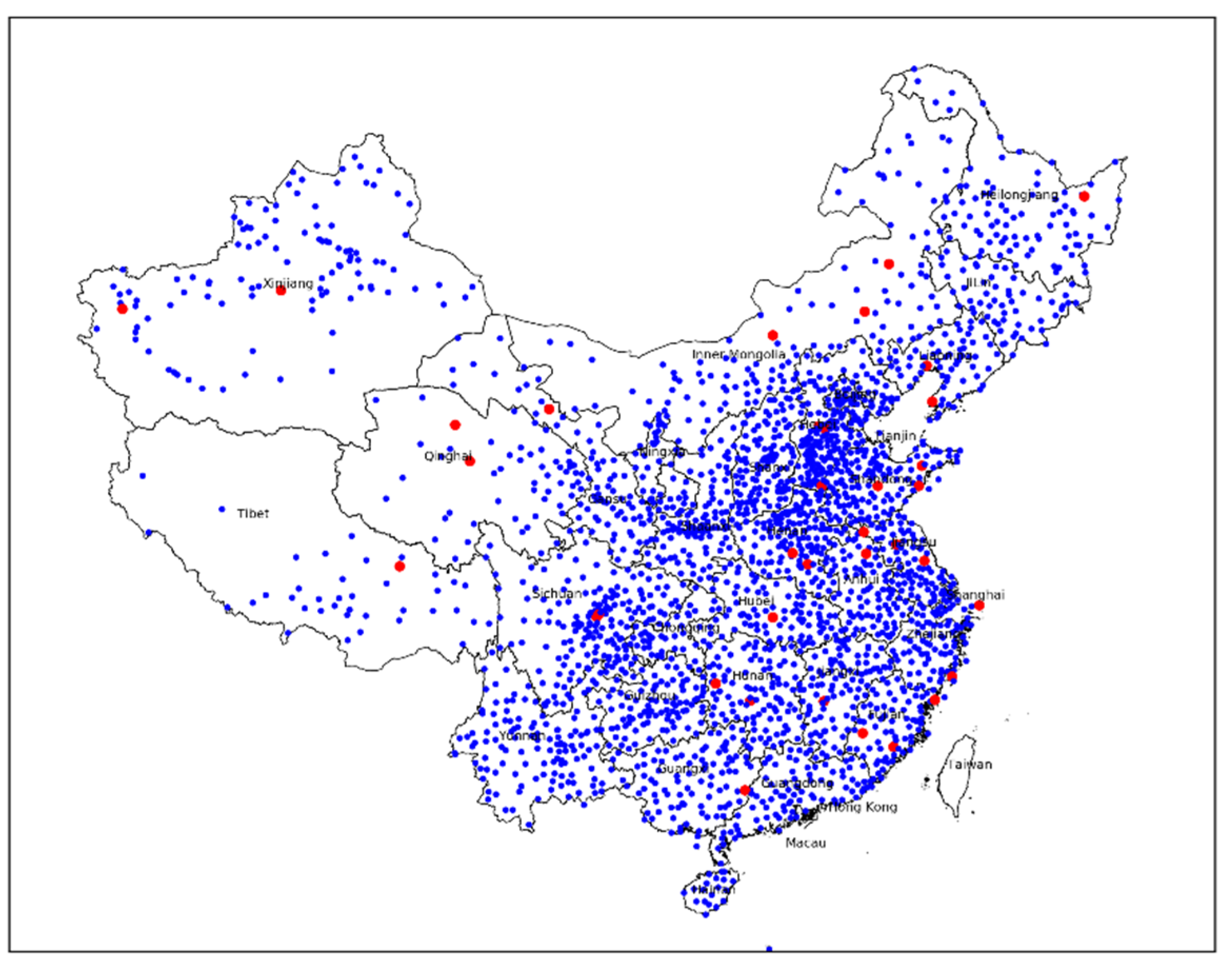
The data employed in this study comprised monthly precipitation data (the daily cumulant in a natural month) acquired from 2416 meteorological observatories covering the period from 1961 to 2019 (the length of the sequence without missing data was greater than 30 years) and 51,062 regional automatic precipitation observation stations from 2015 to 2019, provided by the National Climate Center of China Meteorological Administration. The spatial distribution of the stations is shown in Figure 1.
Figure 1 shows that the density of sites in the east and west of China is quite different. Statistics show that 91% of the long-sequence stations are located east of 100° E (Figure 1a), and 94% of the short-sequence precipitation observation stations are east of 100° E (Figure 1b). The data we use here are the data after quality control. Based on the methods of the climatological limit value check, regional limit value check, time consistency check and spatial consistency check method, Ren Zhihua et al. [30,31] studied the quality control plan of hourly precipitation data from regional automatic stations nationwide. The results show that the accuracy rate of hourly precipitation data after quality control can reach 98%. Table 1 shows the altitude statistics of short-sequence stations. From the data in Table 1, we can see that most of the sites are below 500 m above sea level, accounting for 62.2%.

2.2. SPI

The SPI is an indicator based on probability. The process employed to calculate this indicator first uses a certain distribution function to fit the precipitation over the same period, and based on the cumulative probability of a certain amount of precipitation, the quantile point of the normal distribution is the size of the SPI index. The gamma distribution is the preferred fitting function. The density function expression for this distribution is as follows:
g ( x ) = 1 β α Γ ( α ) x α 1 e x β  
where α is the shape parameter, β is the scale parameter, x is the amount of precipitation, and Γ ( α ) = 0 y α 1 e y d y is gamma function. The maximum likelihood estimates of the parameters α and β are:
α ^ = 1 4 A ( 1 + 4 A 3 )  
β ^ = x ¯ α ^   ,  
where A = ln ( x ¯ ) ln ( x ) n and n is the sample size.
By integrating Formula (1), which is the distribution function of precipitation G ( x ) , we have the following expression:
G ( x ) = 0 x 1 β α Γ ( α ) x α 1 e x β d x , ( x > 0 )   ,  
where G ( x ) is the probability that the precipitation is less than or equal to x . A precipitation value of 0 may be present in the actual precipitation samples, so the distribution function for precipitation needs to be modified. The corrected distribution function is as follows:
H ( x ) = q + ( 1 q ) G ( x ) ,  
where q represents the probability of the precipitation being 0. According to the standard normal distribution, the probability distribution function is as follows:
Φ ( t ) = t 1 2 π e t 2 2 d t   ,  
where Φ ( t ) is the probability that the random variable is less than or equal to t . The corresponding cumulative probability H ( x ) is calculated according to the actual amount of precipitation. The size of t calculated using the equation: H ( x ) = Φ ( t ) , is the size of the SPI and it is obtained with the following expression.
SPI = t = Φ 1 ( H ( x ) )  
Hence, H ( x ) is transformed to the standard normal random variable t with zero mean and variance one. That is, SPI follows the standard normal distribution. The expression above shows that calculating SPI requires a certain number of precipitation samples, and generally more than 30 years of data [22] to allow the calculation of a relatively stable q value and the two parameters α and β . The SPI is often divided into the categories shown in Table 2 in actual analyses [32].
A positive value in Table 2 indicates that the rainfall is higher than the average in the same period and a negative value indicates that the rainfall is lower than the average in the same period. In addition, the SPI indicator is a standard normalized index, so it has a corresponding relationship with the probability. The third column in Table 2 shows the probability for each category.

2.3. Method for Calculating the Precipitation Distribution Parameters for Stations with Short Sequences

In practice, not all stations have long enough observation data. Therefore, it is not possible to directly calculate the SPI based on historical observation data for sites with short sequences of observation records. According to research [16,29], the precipitation distribution parameters of short-sequence stations can be obtained based on the precipitation distribution parameters of the surrounding long-sequence stations. Three calculation methods are given below.

2.3.1. Nearest Neighbor Substitution Method

The spatial distance between the stations was calculated based on the latitude and longitude data for the stations. Based on the distance information, each short-sequence station can find the nearest long-sequence station. The precipitation distribution parameters for the stations with short sequences were regarded as equivalent to the parameters of the nearest neighbor station with a long sequence.

2.3.2. Regional Average Method

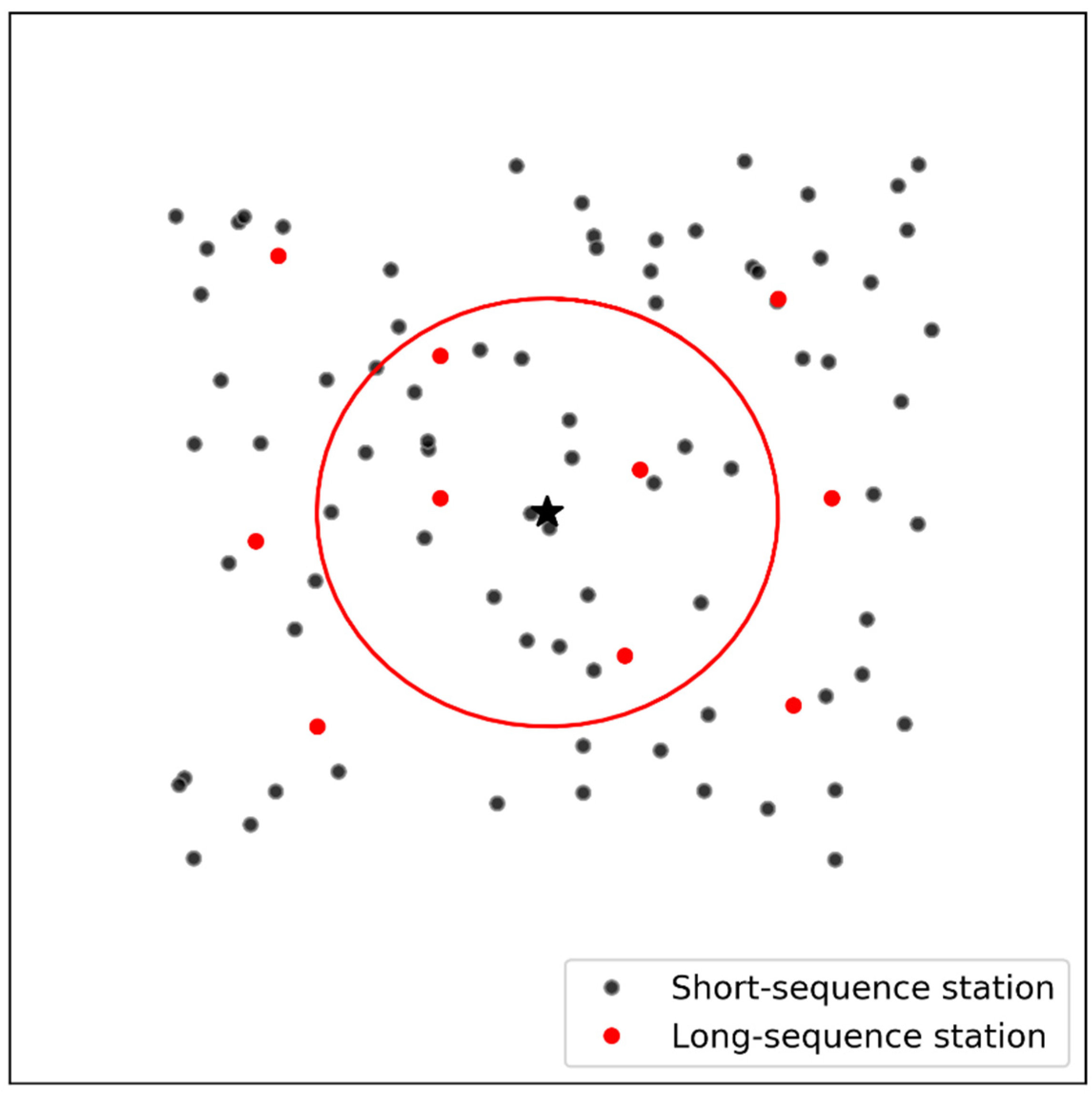
Based on the given value N and the spatial distance information for the stations, the N long-sequence stations could be found around the short-sequence station. The average values for the precipitation distribution parameters at the N long-sequence stations were used to calculate the SPI for the short-sequence station. Figure 2 shows a schematic diagram of solving the distribution parameters of the short-sequence station (marked by a five-pointed star) from the distribution parameters of the surrounding 4 long-sequence stations.

2.3.3. Kriging Interpolation Method

The kriging interpolation method, also known as the spatial autocovariance optimal interpolation method, is widely used in spatial interpolation problems in the field of geo-sciences [33]. The ordinary kriging interpolation method (it is assumed that the semivariance function has a linear relationship with the distance) was applied in a similar manner to the regional averaging method described above for determining the precipitation distribution parameters with the same data.
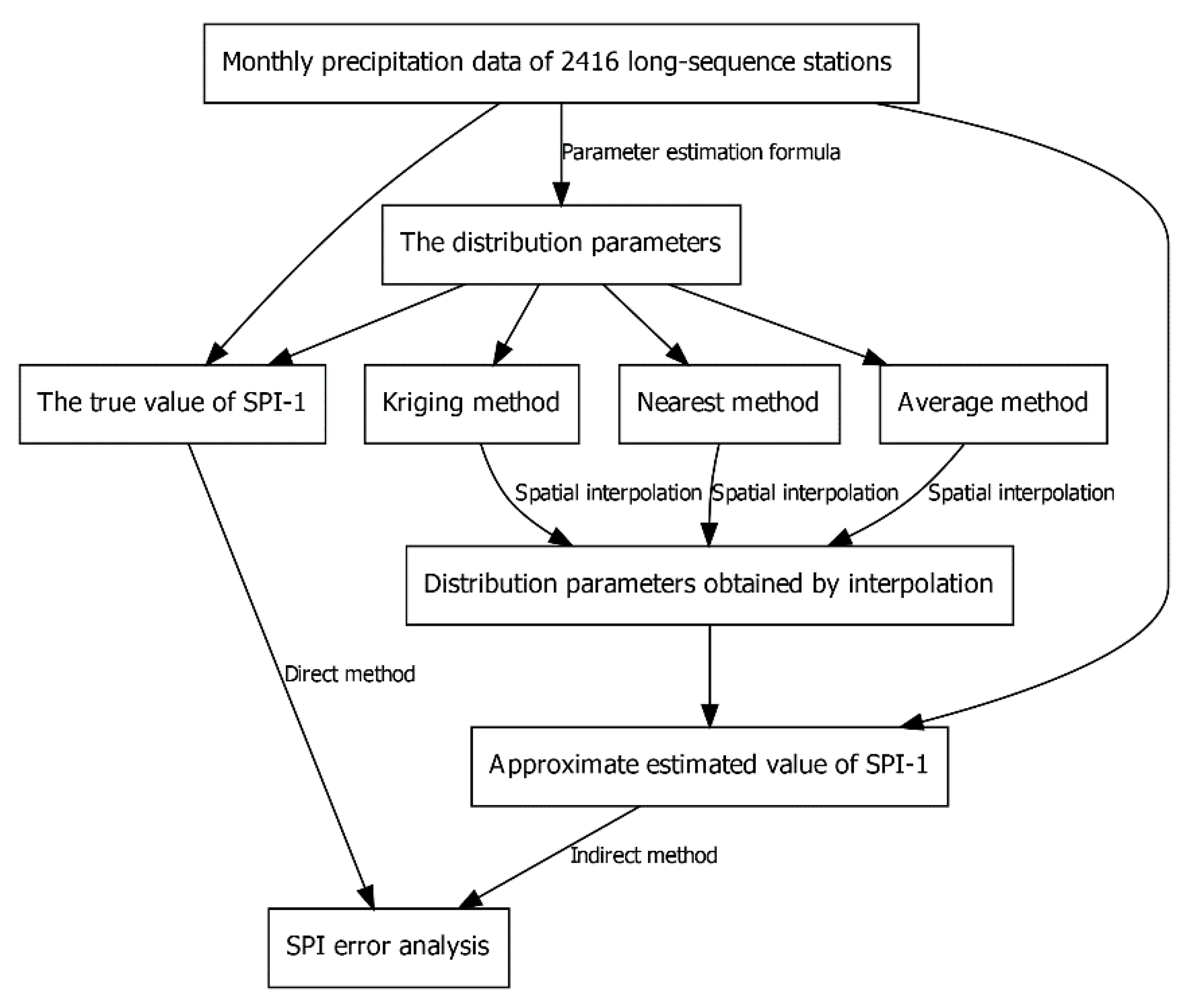
Based on the above three methods, the precipitation distribution parameters of short-sequence stations can be obtained, and then the SPI of short-sequence stations can be realized. It is worth noting that this method does achieve the calculation of SPI, but the error size of SPI and which method can be used to obtain the most accurate SPI is unknown. In order to investigate the reliability of calculating the SPI with short-term precipitation sequences in China, data from 2416 observation stations with long precipitation sequences were used for verification. First, the precipitation distribution parameters and SPI values for each station were obtained based on the real historical data, which were treated as true values. Second, assuming that each long-sequence station is also a short precipitation sequence, the three indirect methods (Section 2.3.1, Section 2.3.2 and Section 2.3.3) were used to obtain the precipitation distribution parameters and SPI values for each station. Then, the SPI obtained by the two ways can be compared, so as to realize the reliability evaluation of the three indirect methods. Finally, based on the best of the three indirect calculation methods, the SPI of more than 50,000 regional automatic stations was obtained and applied to drought monitoring in China, which will be compared with the drought monitoring results obtained from long-sequence stations to verify the actual monitoring effect of high-resolution SPI. A conceptual model illustrating the verification process is shown in Figure 3.

3. Results and Analysis

3.1. The Characteristic Analysis of SPI Error

The monthly precipitation data were fitted using the gamma distribution. Table 3 shows the distribution fitting test based on Kolmogorov–Smirnov (KS) tests.
In SPI calculation, the precipitation distribution function is obtained from the precipitation data of the same month, so it is necessary to check the precipitation distribution of each month. The values given in Table 3 represent the percentage of 2416 sites that passed the KS test. Table 3 shows that except for a few stations, the monthly precipitation at almost all stations was subject to gamma distribution. Taking September as an example, Figure 4 shows the spatial distribution of the KS distribution test at each station.
The results of the KS distribution test for all months showed that most of the sites that failed the KS distribution test were located in North China. When calculating the precipitation distribution parameters of the short-sequence stations, the surrounding long-sequence stations must have the same type of distribution function; otherwise, the spatial interpolation operation cannot be performed. Therefore, consistent precipitation distribution functions and excellent precipitation distribution fitting ability are necessary conditions for subsequent calculations. Table 3 shows that the gamma distribution meets this condition, so this paper selects the gamma distribution as the distribution function of precipitation.
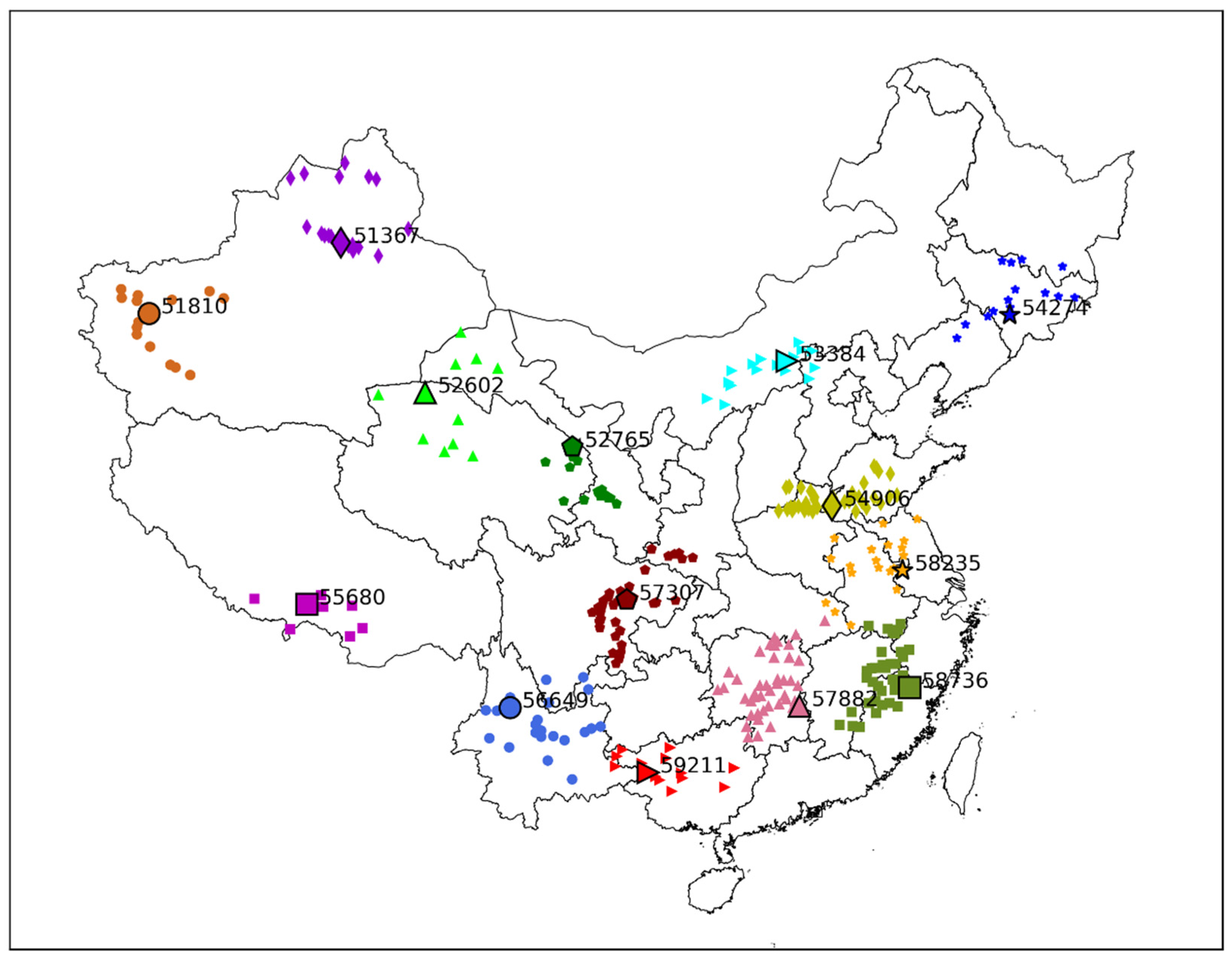
The regional averaging method (Section 2.3.2) and kriging interpolation method (Section 2.3.3) require a predetermined value N to determine the number of surrounding long-sequence stations. Affected by topography and other factors, stations with similar precipitation distribution functions are not necessarily distributed in a circle (for example, band structure). Therefore, the search for long-sequence stations cannot simply follow the circular pattern shown in Figure 2. Due to this, data from 2416 observation stations with long precipitation sequences were used to explore the best calculation strategy for short-sequence stations. The following method is used to search for the long-sequence stations around the short-sequence stations: (1) Use the KS distribution test to determine whether the monthly precipitation of the neighboring stations comes from the same distribution; that is, to determine whether the precipitation distributions of the two stations are similar. The top 50 stations that are closest to the precipitation distribution function of the central station are screened out. (2) The spatial distance between the stations is calculated from the longitude and latitude information of the stations, and the stations with too large a spatial distance in step 1 are eliminated based on the spatial distance information. The maximum distance is set at 400 KM in this paper. Figure 5 shows the stations with similar precipitation distributions as the representative stations (in Figure 1a) in September.
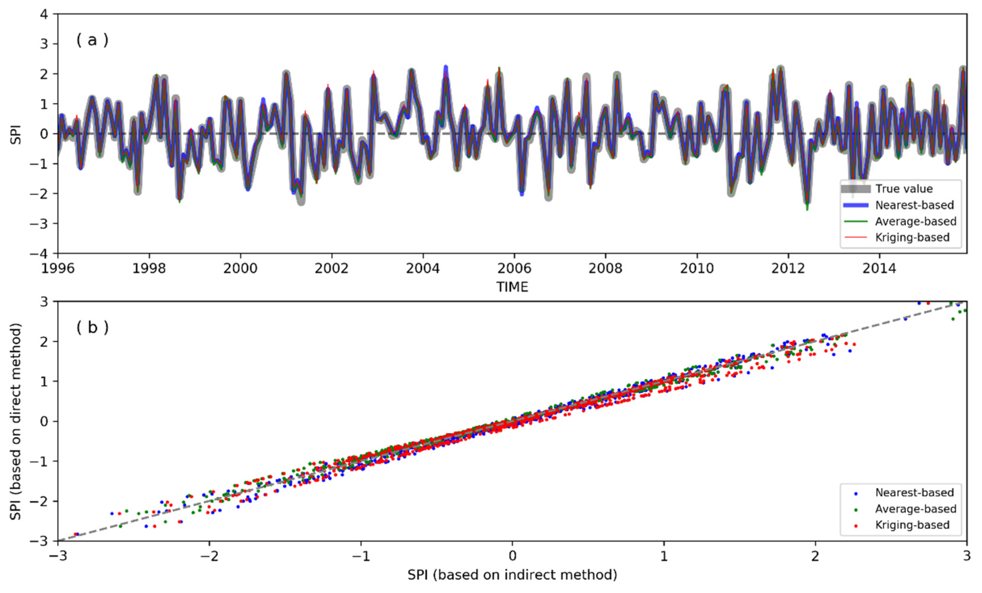
From the results in Figure 5, the stations with similar precipitation distributions are mostly located near the representative stations, and they are not evenly distributed in the circle. Based on these stations, the precipitation distribution parameters of each representative station can be obtained using the method introduced in Section 2.3, and then the SPI sequence can be obtained. We take station 54,906 in Figure 1a as an example, and Figure 6 shows the SPI sequence based on three methods.
According to the comparison of SPI sequence in Figure 6a, SPI calculated based on different indirect methods had very similar sizes. Large errors are likely to occur at the peak value of the sequence. To further verify this result, a comparative analysis of SPI is presented in Figure 6b. The Y-coordinate value in Figure 6b represents the true value of SPI, and the X-coordinate value represents the SPI calculated based on different indirect methods. Therefore, the more accurate the value of SPI calculated based on the indirect method is, the closer the position of scatter points is to the diagonal line in Figure 6b. According to the scatter distribution in Figure 6b, the SPI value of station 54,906 obtained based on the three indirect methods is almost equal to the true value of SPI. In the whole country, whether the SPI based on the indirect method can be approximately equal to the true value is of great significance. Similar to the calculation in Figure 5 and Figure 6, we calculated the SPI sequence of all stations across the country based on three indirect methods. Compared with the true value of SPI, the error sequence of SPI is obtained, and the standard deviation (STD) of the SPI error sequence is obtained. The larger the standard deviation, the less accurate the SPI calculated by the indirect method, so this value can be used as an analysis of the SPI calculation error. Figure 7 shows the spatial distribution of the STD of SPI error across the country.
As shown in Figure 7, the spatial distribution characteristics of SPI errors obtained based on different indirect methods were very consistent, which all showed that the SPI error in eastern China was small and the SPI error in western China was large. In most areas of eastern China, the STD of the SPI error was less than 0.2. Among the three indirect calculation methods, the nearest neighbor substitution method performed better than the other two methods in some areas of western China, but its performance in most areas was inferior to those of the other two methods. The difference in the performance of the regional average method and kriging method was not obvious in eastern China. However, in the western region, the nearest neighbor substitution method performed better than the other two methods in some regions. Since the calculation of the distribution parameters of short-sequence stations completely depends on the surrounding long-sequence stations, the closer to the long-sequence stations, the more accurate the indirect calculation of SPI. Due to the dense distribution of long-sequence stations in the east (Figure 1a), the average distance from short-sequence stations to long-sequence stations in the east is much lower than the value in the west. It is for this reason that no matter which indirect calculation method is adopted in the eastern region, the error of SPI east of 100° E is significantly lower than the error of SPI west of 100° E. The actual applications of the SPI index include two ways: analysis based directly on the size of the SPI index and analysis based on drought categories (Table 2). Therefore, Figure 8 showed the spatial distribution of the accuracy of SPI classification.
As shown in Figure 8, the spatial distribution structure was consistent with the spatial distribution structure for the SPI error (Figure 7). The accuracy of SPI classification in the eastern region was higher than the accuracy in the western region. The accuracy of SPI classification in most of eastern China was higher than 80%, but in parts of western China, it was lower than 60%. From the perspective of the size of the SPI error (Figure 7) and the accuracy of the SPI classification (Figure 8), the calculation of high-resolution SPI in the eastern region would be more accurate.
Although the error of SPI in eastern China was mostly less than 0.2 and the accuracy of SPI classification could reach 80%, did this error fall within an acceptable range? In order to further analyze the credibility of the indirect methods, the resampling method was used to discuss how much error is acceptable. As we all know, it is recommended to use a longer precipitation sample period to calculate the SPI value [34,35] but sufficient observation data might not be available for a long period, so the calculation is generally based on a 30-year sample. However, due to randomness, the SPI index calculated by different 30-year precipitation samples is not consistent. Therefore, the SPI error due to the 30-year sample should be regarded as a tolerable error limit. Based on the precipitation data of each station, the resampled data of each station with 30 groups of precipitation data containing 30 years was obtained by using the resampling method. Based on the resampled data, the STD of the SPI error and the accuracy of SPI classification can be calculated, which is regarded as the error tolerance limit. The result showed that the average value of STD was almost 0.27 nationwide and the accuracy of SPI classification was almost 76%. Therefore, it is feasible and acceptable to calculate the SPI based on indirect methods in eastern China and the western region where the stations are concentrated.

3.2. The Reason Analysis of the SPI Error and the Drought Monitoring Examples

According to the SPI calculation principle introduced in Section 2.2, the error of SPI based on indirect methods was entirely due to the error of distribution parameters. Since the precipitation distribution function was calculated separately for each month, the errors of precipitation distribution parameters in different months were not consistent. Taking January as an example, Figure 9 shows the spatial distribution of parameter errors.
From the analysis in Section 3.1, it could be seen that the kriging method was better than the other two indirect methods, so Figure 9 only showed the results based on the kriging method. The value in Figure 8 is the rate of change compared to the real value (take parameter α as an example: the value in Figure 9 a is calculated based on α i n d i r e c t α d i r e c t α d i r e c t × 100 % ). As shown in Figure 9, the distribution parameters β and q had much greater changes than α , with increases of 30% in western China. The parameter error analysis of other months shows that the error of the distribution parameters has obvious seasonal characteristics, and the results show that the error is the smallest in summer and the largest in winter. In addition, the error of the distribution parameter α has the smallest change with the season, and parameter q has the largest change. Therefore, the estimation error of the distribution parameters β and q is the most important cause of SPI error.
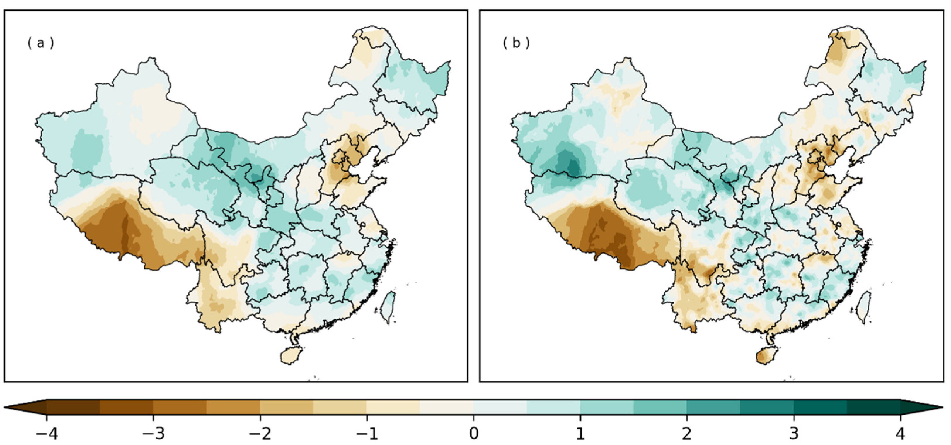
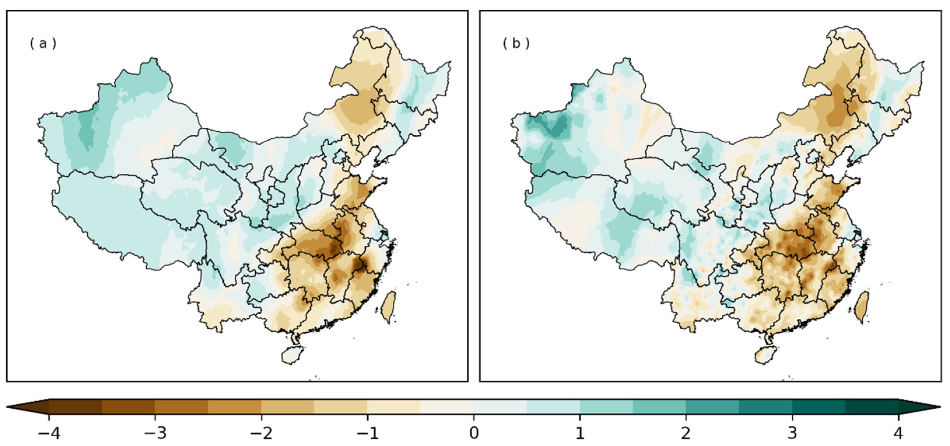
The previous SPI error analysis based on 2416 long-sequence stations shows that it is feasible to develop high-resolution SPI indicators in eastern China. For the SPI calculation of 51,062 short-sequence stations, firstly, the long-sequence station nearest to the short-sequence station is searched based on the longitude and latitude information. Secondly, based on the best indirect method of calculating the distribution parameters of the long-sequence station (based on the results in Figure 7), the precipitation distribution parameters of the 51,062 short-sequence station are solved. Figure 10 and Figure 11 shows the comparison of drought monitoring results in China.
Figure 10 and Figure 11 show that the monitoring results obtained based on different data are very consistent, and the results obtained based on 51,062 stations are more detailed than those obtained based on 2416 stations. The above results once again verify that it is feasible to carry out the calculation of the high-resolution SPI index in eastern China. It needs to be pointed out that it may be due to the error of indirect calculation of distribution parameters in winter and spring. The monitoring results during this period have certain errors, but the results in southern China and other seasons are consistent. The comparative analysis of drought monitoring over many months shows that it is reliable to carry out SPI calculations for short-sequence stations in various seasons in southern China and in the summer (autumn) season in most parts of China.

4. Summary and Discussion

In this study, in order to facilitate SPI calculations with short-term precipitation data, long-term precipitation data from 2416 stations in China were used to conduct a feasibility analysis. The results showed that it is feasible to calculate the SPI indirectly in eastern China. The SPI error was small in east China and large in west China, and the SPI was more accurate when the observation stations were denser. The standard deviation of the SPI error in eastern China was generally less than 0.2 and the category agreement lager than 80%, which was lower than the error using the 30-year precipitation samples. Error analysis showed that the kriging method and regional average method performed better than the nearest neighbor substitution method. The reason for the SPI error is the error generated by the indirect method to solve the distribution parameters, especially the distribution parameters β and q have the largest errors and seasonal differences. The analysis of two examples in China shows that the SPI distribution of 51,062 stations obtained by the indirect method is in good agreement with the results based on 2416 stations, which verifies that the calculation of SPI based on a short series of precipitation data in eastern China is reliable. However, it should be noted that during the winter and spring seasons, short-sequence stations in northern China have certain errors in the calculation of SPI.
As the precipitation distribution parameters are calculated from decades of precipitation data, they are susceptible to the impact of climate change, especially the stations on the boundary of the climate zone. Besides, the precipitation distribution parameters are obtained based on the precipitation data of the same month, so the spatial distribution of the precipitation distribution parameters in different months is not consistent. However, in the same season, the spatial distribution of the distribution parameters is relatively consistent. Therefore, the SPI is prone to large errors in the months of seasonal transition. On the other hand, due to the obvious seasonal rainfall in China, the parameter q is almost always 0 in the rainy season, so there is almost no interpolation error in this season. However, in the non-rainy season, local precipitation is often affected by topography or other factors, so the spatial distribution of parameter q is not smooth. For this reason, the interpolation error of q in the non-rainy season is relatively large, which further affects the calculation accuracy of SPI.
The SPI is a drought index with multiple time scales, but the present study only investigated the SPI on a monthly scale, and it did not verify the accuracy of the SPI with time scales of 3, 6, 12, and 24 months. However, it is considered that when the time scale is larger, the error will be smaller when using an indirect method to obtain the SPI because the spatial difference in rainfall will be lower over a longer time scale. All of the analyses conducted in this study were based on the gamma distribution function, but this function is not the best function for fitting the precipitation at all stations, and thus the SPI error could be affected by the distribution function selected. In addition, the same distribution function must be assumed when indirect methods are employed to determine the precipitation distribution parameters; otherwise, the SPI index cannot be calculated.

Author Contributions

Methodology, D.Z., W.H. and Q.Z.; writing original draft preparation, D.Z. and P.Y.; writing review and editing, Q.Z. and W.H.; visualization, D.Z., H.W. and P.Y. All authors have read and agreed to the published version of the manuscript.

Funding

This work was funded by the National Key Research and Development Program of China (Grant:2017YFC1502402), the National Natural Science Foundation of China (Grant: 41775078, 42005058), the Natural Science Research Project of Higher Education in Jiangsu Provinces (Grant: 20KJB170004) and school-level research projects of Yancheng Institute of Technology (Grant: xjr2019052).

Institutional Review Board Statement

Not applicable.

Informed Consent Statement

Not applicable.

Data Availability Statement

The data of more than 2000 stations can be downloaded from China Meteorological Data Center (https://data.cma.cn, accessed on 5 May 2021); further inquiries can be directed to the corresponding author/s.

Conflicts of Interest

The authors declare no conflict of interest.

References

  1. Wilhite, D.A. Drought and Water Crises: Science, Technology, and Management Issues; CRC Press: Boca Raton, FL, USA, 2005. [Google Scholar]
  2. Huang, S.; Huang, Q.; Chang, J.; Leng, G. Linkages between hydrological drought, climate indices and human activities: A case study in the Columbia River basin. Int. J. Climatol. 2016, 36, 280–290. [Google Scholar] [CrossRef]
  3. Fang, W.; Huang, S.; Ren, K.; Huang, Q.; Huang, G.; Cheng, G.; Li, K. Examining the applicability of different sampling techniques in the development of decomposition-based streamflow forecasting models. J. Hydrol. 2019, 568, 534–550. [Google Scholar] [CrossRef]
  4. Zhang, Q.; Yao, Y.; Li, Y.; Huang, J.; Ma, Z.; Wang, Z.; Wang, S.; Wang, Y.; Zhang, Y. Causes and Changes of Drought in China: Research Progress and Prospects. J. Meteorol. Res. 2020, 34, 460–481. [Google Scholar] [CrossRef]
  5. Hänsel, S.; Ustrnul, Z.; Łupikasza, E.; Skalak, P. Assessing seasonal drought variations and trends over Central Europe. Adv. Water Resour. 2019, 127, 53–75. [Google Scholar] [CrossRef]
  6. Huang, J.; Yi, Y.; Wang, S.; Chou, J. An analogue-dynamical long-range numerical weather prediction system incorporating historical evolution. Q. J. R. Meteorol. Soc. 1993, 119, 547–565. [Google Scholar]
  7. Jenkins, K.; Warren, R. Quantifying the impact of climate change on drought regimes using the Standardised Precipitation Index. Appl. Clim. 2015, 120, 41–54. [Google Scholar] [CrossRef] [Green Version]
  8. Hao, Z.C.; Hao, F.H.; Singh, V.P.; Ouyang, W. Quantitative risk assessment of the effects of drought on extreme temperature in eastern China. J. Geophys. Res.-Atmos. 2017, 122, 9050–9059. [Google Scholar] [CrossRef]
  9. Chamani, R.; Monkam, D.; Djomou, Z.Y. Analysis of return periods and return levels of Yearly July-September extreme droughts in the West African Sahel. Clim. Dyn. 2019, 52, 3421–3433. [Google Scholar] [CrossRef]
  10. Zhang, Q.; Han, Y.Y.; Zhang, L.Y.; Wang, J.S. Analysis on the Character and Management Strategy of Drought Disaster and Risk under the Climatic Warming. Adv. Earth Sci. 2014, 29, 80–91. (In Chinese) [Google Scholar]
  11. Wang, Y.; Zhao, W.; Zhang, Q.; Yao, Y.B. Characteristics of drought vulnerability for maize in the eastern part of Northwest China. Sci. Rep. 2019, 9, 1–9. [Google Scholar]
  12. Svoboda, M.; LeComte, D.; Hayes, M.; Heim, R.; Gleason, K.; Angel, J.; Rippey, B.; Tinker, R.; Palecki, M.; Stooksbury, D. The drought monitor. Bull. Am. Meteorol. Soc. 2002, 83, 1181–1190. [Google Scholar] [CrossRef] [Green Version]
  13. Venkataraman, K.; Tummuri, S.; Medina, A.; Perry, J. 21st century drought outlook for major climate divisions of Texas based on CMIP5 multimodel ensemble: Implications for water resource management. J. Hydrol. 2016, 534, 300–316. [Google Scholar] [CrossRef] [Green Version]
  14. Liu, S.; Huang, S.; Xie, Y.; Huang, Q.; Leng, G.; Hou, B.; Zhang, Y.; Wei, X. Spatial-temporal changes of maximum and minimum temperatures in the Wei River Basin, China: Changing patterns, causes and implications. Atmos. Res. 2018, 204, 1–11. [Google Scholar] [CrossRef]
  15. Dow, K.; Murphy, R.L.; Carbone, G.J. Consideration of User Needs and Spatial Accuracy in Drought Mapping. J. Am. Water Resour. Assoc. 2009, 45, 187–197. [Google Scholar] [CrossRef]
  16. DeGaetano, A.T.; Belcher, B.N.; Noon, W. Temporal and spatial interpolation of the standardized precipitation index for computational efficiency in the dynamic drought index tool. J. Appl. Meteorol. Climatol. 2015, 54, 795–810. [Google Scholar] [CrossRef]
  17. Wilhite, D.A.; Sivakumar, M.V.; Pulwarty, R. Managing drought risk in a changing climate: The role of national drought policy. Weather Clim. Extrem. 2014, 3, 4–13. [Google Scholar] [CrossRef] [Green Version]
  18. Mishra, A.K.; Singh, V.P. A review of drought concepts. J. Hydrol. 2010, 391, 202–216. [Google Scholar] [CrossRef]
  19. Council, A. AMS statement on meteorological drought. Bull. Am. Meteorol. Soc. 2004, 85, 771–773. [Google Scholar]
  20. Huang, S.; Li, P.; Huang, Q.; Leng, G.; Hou, B.; Ma, L. The propagation from meteorological to hydrological drought and its potential influence factors. J. Hydrol. 2017, 547, 184–195. [Google Scholar] [CrossRef]
  21. Zhang, Q.; Zhang, L.; Cui, X.C.; Zeng, J. Progresses and challenges in drought assessment and monitoring. Adv. Earth Sci. 2011, 26, 763–778. (In Chinese) [Google Scholar]
  22. McKee, T.B.; Doesken, N.J.; Kleist, J. The relationship of drought frequency and duration to time scales. In Proceedings of the 8th Conference on Applied Climatology, Anaheim, CA, USA, 17–22 January 1993; pp. 179–183. [Google Scholar]
  23. Zhang, Q.; Xu, C.Y.; Zhang, Z.X. Observed changes of drought/wetness episodes in the Pearl River basin, China, using the standardized precipitation index and aridity index. Appl. Clim. 2009, 98, 89–99. [Google Scholar] [CrossRef]
  24. Yang, P.; Xia, J.; Zhan, C.; Zhang, Y.; Hu, S. Discrete wavelet transform-based investigation into the variability of standardized precipitation index in Northwest China during 1960–2014. Appl. Clim. 2018, 132, 167–180. [Google Scholar] [CrossRef]
  25. Odewale, O.; Adebola, A. Integration of standardized precipitation index and drought severity index for assessment of drought in the Sudano-Sahelian ecological zone of Nigeria. Clim. Chang. 2019, 5, 188–199. [Google Scholar]
  26. Hayes, M.; Svoboda, M.; Wall, N.; Widhalm, M. The Lincoln declaration on drought indices: Universal meteorological drought index recommended. Bull. Am. Meteorol. Soc. 2011, 92, 485–488. [Google Scholar] [CrossRef] [Green Version]
  27. Hao, Z.; Yuan, X.; Xia, Y.; Hao, F.; Singh, V.P. An overview of drought monitoring and prediction systems at regional and global scales. Bull. Am. Meteorol. Soc. 2017, 98, 1879–1896. [Google Scholar]
  28. World Meteorological Organization. Standardized Precipitation Index User Guide; World Meteorological Organization: Geneva, Switzerland, 2012. [Google Scholar]
  29. McRoberts, D.B.; Nielsen-Gammon, J.W. The Use of a High-Resolution Standardized Precipitation Index for Drought Monitoring and Assessment. J. Appl. Meteorol. Climatol. 2012, 51, 68–83. [Google Scholar] [CrossRef]
  30. Ren, Z.H.; Zhao, P.; Zhang, Q.; Zhang, Z.F.; Cao, L.J.; Yang, Y.R.; Zou, F.L.; Zhao, Y.F.; Zhao, H.M.; Chen, Z. Quality contral procedured for hourly precipitaion data from automatic weather stations in China. Meteorol. Mon. 2010, 36, 123–132. (In Chinese) [Google Scholar]
  31. Ren, Z.H.; Zhang, Z.F.; Sun, C.; Liu, Y.M.; Li, J.; Ju, X.H.; Zhao, Y.F.; Li, Z.P.; Zhang, W.; Li, H.K.; et al. Development of three-step quality control system of real-time observation data from AWS in China. Meteorol. Mon. 2015, 41, 1268–1277. (In Chinese) [Google Scholar]
  32. Lloyd-Hughes, B.; Saunders, M.A. A drought climatology for Europe. Int. J. Climatol. 2002, 22, 1571–1592. [Google Scholar]
  33. Elbasiouny, H.; Abowaly, M.; Abu_Alkheir, A.; Gad, A. Spatial variation of soil carbon and nitrogen pools by using ordinary Kriging method in an area of north Nile Delta, Egypt. Catena 2014, 113, 70–78. [Google Scholar]
  34. Wu, H.; Hayes, M.J.; Wilhite, D.A.; Svoboda, M.D. The effect of the length of record on the standardized precipitation index calculation. Int. J. Climatol. A J. R. Meteorol. Soc. 2005, 25, 505–520. [Google Scholar] [CrossRef] [Green Version]
  35. Carbone, G.; Lu, J.; Brunetti, M. Estimating uncertainty associated with the standardized precipitation index: Estimating uncertainty associated with the SPI. Int. J. Climatol. 2018, 38, 607–616. [Google Scholar] [CrossRef]
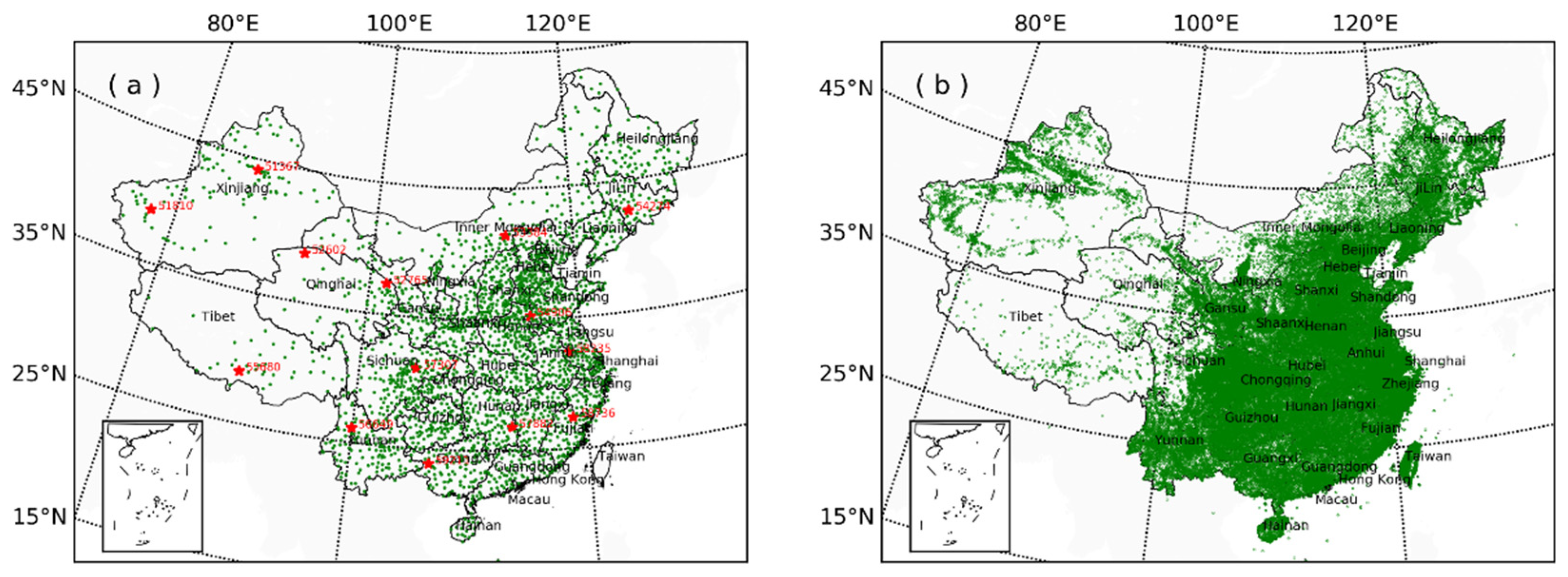
Figure 1. Spatial distribution of meteorological observation stations. (a) The long-term precipitation stations. (b) The short-term precipitation stations. The red five-pointed stars in Figure 1a denote the selected representative stations.
Atmosphere 12 00603 g001
Figure 2. Schematic diagram illustrating the regional average method.
Atmosphere 12 00603 g002
Figure 3. Conceptual model of the verification process.
Atmosphere 12 00603 g003
Figure 4. The KS test in September. The red dots indicate sites that have not passed the KS distribution test.
Atmosphere 12 00603 g004
Figure 5. The stations with similar precipitation distributions as the representative stations in September.
Atmosphere 12 00603 g005
Figure 6. Comparison of real SPI values for station 54,906 with values obtained using different indirect methods. (a) SPI time series; (b) SPI-SPI plot.
Atmosphere 12 00603 g006
Figure 7. The spatial distribution of STD of SPI error. (a) Nearest neighbor substitution method; (b) regional average method; (c) kriging method.
Atmosphere 12 00603 g007
Figure 8. The spatial distribution of the accuracy of SPI classification. (a) Nearest neighbor substitution method; (b) regional average method; (c) kriging method.
Atmosphere 12 00603 g008
Figure 9. The spatial distribution of parameter errors. (a) α ; (b) β ; (c) q .
Atmosphere 12 00603 g009
Figure 10. The comparison of drought monitoring based on SPI index Jun 2019. (a) Based on 2416 stations; (b) based on 51,062 stations.
Atmosphere 12 00603 g010
Figure 11. The comparison of drought monitoring based on SPI index in September 2019. (a) Based on 2416 stations; (b) based on 51,062 stations.
Atmosphere 12 00603 g011
Table 1. Altitude statistics of short-sequence stations.
Altitude (Meter)Proportion (%)
H ≤ 209.5
20 < H ≤ 5011.5
50 < H ≤ 10010.3
100 < H ≤ 20011.7
200 < H ≤ 50019.2
500 < H ≤ 100014.5
1000 < H ≤ 200017.4
2000 < H ≤ 30003.9
3000 < H2.0
Table 2. The classification of drought categories and corresponding probability [32].
SPI ValueCategoryProbability
2.00 ≤ SPIExtremely wet0.023
1.50 ≤ SPI ≤ 1.99Severely wet0.044
1.00 ≤ SPI ≤ 1.49Moderately wet0.092
0.00 ≤ SPI ≤ 0.99Mildly wet0.341
−0.99 ≤ SPI ≤ 0.00Mild drought0.341
−1.49 ≤ SPI ≤ −1.00Moderate drought0.092
−1.99 ≤ SPI ≤ −1.5Severe drought0.044
SPI ≤ −2.00Extreme drought0.023
Table 3. Fitting test results of precipitation distribution.
MonthJan.Feb.Mar.Apr.MayJuneJulyAug.Sept.Oct.Nov.Dec.
Proportion (%)93.794.396.297.398.798.398.898.798.596.093.393.6
Publisher’s Note: MDPI stays neutral with regard to jurisdictional claims in published maps and institutional affiliations.